Impacts of Rainstorm Characteristics on Runoff Quantity and Quality Control Performance Considering Integrated Green Infrastructures

Abstract

Green infrastructure (GI) has been implemented globally to mitigate the negative effects of urbanization. GI also regulates the urban runoff process and reduces non-point source pollution by intercepting initial runoff pollution and stormwater storage. In this paper, the impacts on GI were quantified and analyzed, considering eight designed storms with a 24 h duration and eight others with a 2 h duration with the combination of two characteristics (return period and peak time). The runoff process and reduction effect of pollutants were simulated for GI combinations (green roofs, vegetative swale, bio-retention units, and permeable pavement) using the Storm Water Management Model, taking the Dongshan campus of Shanxi University as an example case study. The results show that the GI combination can reduce runoff, suspended solids (SS), and chemical oxygen demand (COD). For short- and long-duration rainstorms, the average reduction rates of runoff, SS, and COD were 39.7%, 38.8%, and 39.6%, and 36.5%, 31.7%, and 32%, respectively, indicating its better effectiveness for short-duration storms. The GI’s effect was more sensitive during the short-duration storms owing to the greater absolute value of the 2 h elastic coefficients versus that of the 24 h, and the best reduction effect was observed with a rainfall peak coefficient of 0.1. These results provide a scientific reference for GI planning and implementation under a changing climate in the future.

1. Introduction

The expansion of cities has occurred in recent decades, and the trend continues. It is reported that by 2050, two-thirds of the world’s population will be in cities [1], and China’s urbanization rate will exceed 80% [2]. The increased impervious surface in cities has altered the original hydrological path and caused a series of urban water problems, such as urban waterlogging and non-point source pollution [3,4,5]. Due to the adverse effects of rapid urbanization, urban rainfall-runoff system management has become the focus of the government and experts.

To manage the urban water problems, many countries have proposed solutions, such as Best Management Practices in the United States, Water Sensitive Urban Design in Australia, and Sponge City (SPC) in China [6,7,8]. Although these solutions are distinctive, they all regard green infrastructure (GI) as essential [9,10,11,12]. Compared with the traditional drainage system, which removes water quickly, GI can collect rainwater from the source, reduce runoff, and improve water quality [13,14]. The hydrological and environmental benefits of GI are usually achieved through green roofs (GR), vegetative swale (VS), bio-retention units (BR), permeable pavement (PP), and other green measures [15].

These GIs’ benefits have been confirmed by field studies [16,17,18], laboratory experiments [19], and modeling simulations [10,20,21,22,23]. The effectiveness of GI practices can be measured by several indexes, such as flood control and pollution reduction, by comparing a base case with various scenarios [9]. In addition, the analytical probabilistic method is used to quantify the runoff reduction effect of GR [24] and BR [25], which often takes the water retention capacity as the index. With the deepening of GIs’ research, many tools are available to simulate the effects of GI practices. For example, the Analytical Stormwater Models (ASMs) [26] and GI Flexible Model (GIFMod) [27] can be used to evaluate a wide range of GIs’ performance according to a user’s demand. Some models can analyze the performance of GI practices in large catchment-scale basins through preset modules, such as the Storm Water Management Model (SWMM), the Soil and Water Assessment Tool (SWAT) [28], the System for Urban Stormwater Treatment and Analysis Integration (SUSTAIN), and the Model for Urban Stormwater Improvement Conceptualization (MUSIC) [25]. In addition, Zhang and Guo [29] provided an alternative method based on the basic SWMM algorithm, which can be applied to models that do not have LID modules.

As an open-source model, SWMM is one of the most advanced and popular models for water quality and quantity simulation in urban water system management [30]. Since the low impact development (LID) module was added to the SWMM, it has been applied to evaluate the hydrological and environmental benefits of GI [20,31,32,33]. Tang et al. [33] analyzed the SWMM’s robustness in stormwater quality modeling based on intensive field monitoring data, demonstrating that it is feasible to simulate runoff pollutants using SWMM in the design of Sponge Cities.

In the context of climate change and rapid urbanization, extreme precipitation occurs frequently, which poses the potential threat of flooding and runoff pollution to urban safety. The impact of different rainfall characteristics on the GIs’ effect has aroused researchers’ attention in recent years. Many studies pay attention to the impact of different rainfall characteristics on runoff reduction of GIs [34,35,36,37]. Previous studies have found that the effect of runoff mitigation decreases as the return period increases [38,39,40]. Furthermore, there is no unified understanding of the impact of time to peak on the GI effect due to the different indicators and GI scenarios [38,41,42]. Studies on rainfall duration are mostly limited to short-duration rainstorms (≤6 h) [41,42]. In terms of the pollutant reduction effect, many studies have analyzed the performance of GI under different return periods [43,44,45]. In addition, the design of the rainfall process mainly relies on the rainstorm intensity formula, which is more suitable for the design of a short-duration rainstorm process. Therefore, it is necessary to find a new way to design a long-duration rainstorm process to explore further the impact of rainstorm characteristics change on GIs’ effects under the background of frequent extreme precipitation and the general construction of Sponge City.

In this study, we established the urban hydrologic and hydrodynamic models in the Dongshan campus of Shanxi University as an example to assess GI’s efficacy. Short- and long-duration rainstorms were designed according to different methods and return periods and rain peak coefficients were also taken into consideration. Changes in runoff and pollutants under 16 rainstorms were simulated to explore the performance of GI in the long-duration rainstorm process and the difference between long-duration and short-duration rainstorms. The findings are expected to support GI planning and provide insights for rainwater management in the future.

2. Methods and Materials

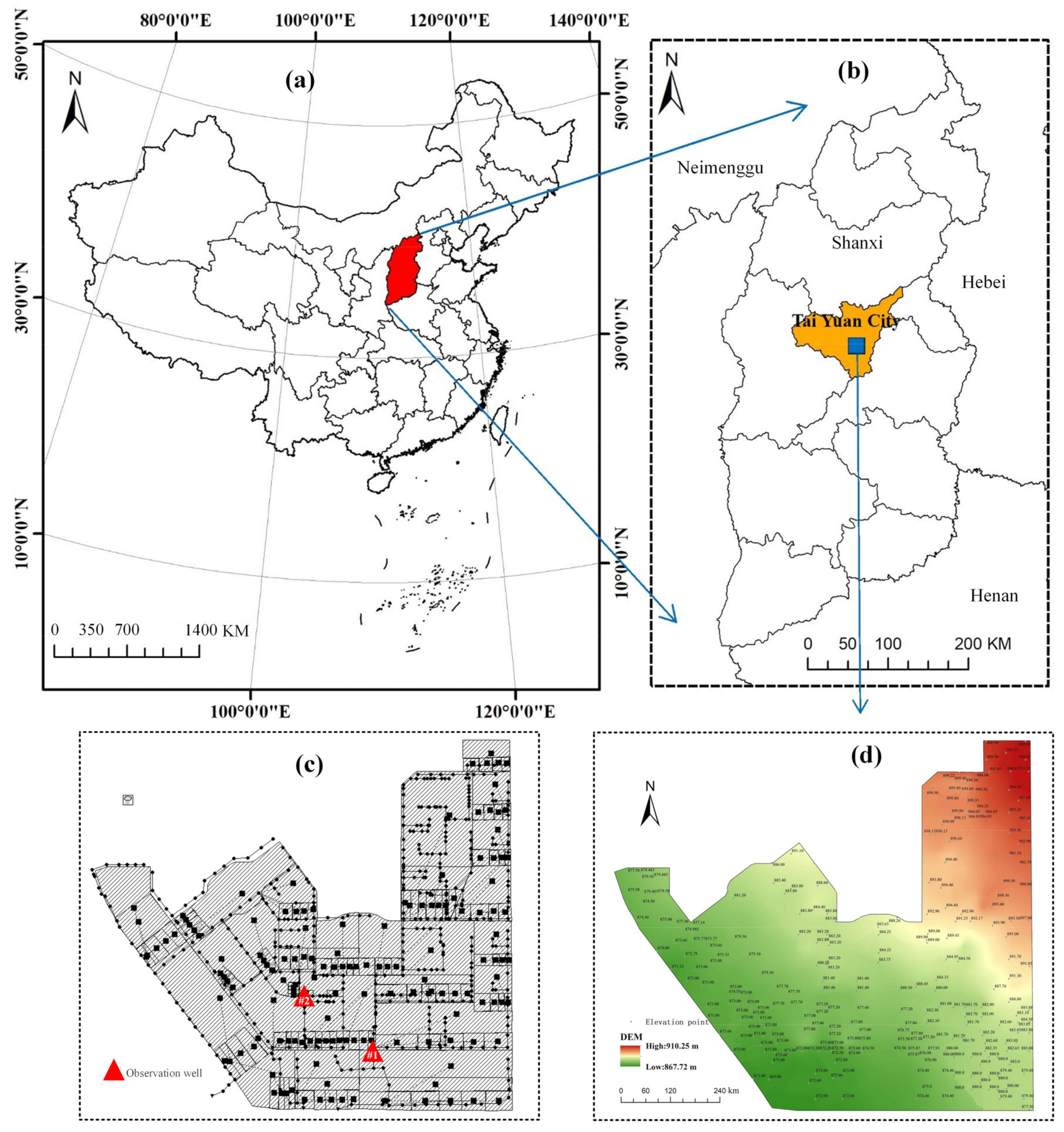
2.1. Study Area and Data

The Dongshan campus of Shanxi University was selected as the case study. It is located in the southeast of Taiyuan City, China (Figure 1). The campus is currently in the first stage of construction with an area of about 0.52 km², which provides convenient conditions for the layout of GI. The campus’s overall terrain is undulating, and the basic trend is higher in the east and lower in the west, higher in the north and lower in the south. The region has a warm, temperate continental monsoon climate; the average annual rainfall is 444.4 mm (1951–2016). The rainy season is from June to September, accounting for approximately 73% of the annual rainfall.

The data used in this study includes data on land use, elevation, and rainwater pipe network, all of which are important for constructing models. All data were obtained from the campus construction plan. According to the plan, the main types of land use on campus are ground, building, roads, and green space. The elevation points of the study area are shown in Figure 1d. The spatial distribution of elevation in the study area was obtained by Kriging interpolation.

2.2. Scenarios Design

2.2.1. Rainstorm Scenarios

The total amount, time to peak, and duration are three important characteristics of designed rainfall events [46]. In this study, the amount of rainfall was represented by the return period (P); the peak time was represented by the rainfall peak coefficient (R), which is the ratio of the time before peak intensity appears to the total rainfall time; and the rainfall duration (T) refers to the time from the beginning to the end of the rainfall. Two rainstorm series were designed to compare the performance of GI combinations between short-duration (2 h) and long-duration (24 h) storms. Each series contains four rainstorms with a 5-, 10-, 20-, 50-year return period and four rainstorms with peak coefficients of 0.1, 0.4, 0.6, and 0.9. The short-duration rainstorms were generated by the Chicago design storm pattern according to the rainstorm intensity formula of Taiyuan City, which is described as Equation (1) [47].

$$q=\frac{1446.22(1+0.8671lgP)}{{(t+5)}^{0.796}}$$

(1)

where $q$ is the intensity of the rainstorm, $\mathrm{L}/\left(\mathrm{s}\cdot {\mathrm{hm}}^2\right)$; P is the return period, yr; and t is the rainfall duration, min.

Since the rainstorm intensity formula is more suitable for short-duration rainstorms [48], the long-duration rainstorm processes were designed based on historical rainfall data. The methods are as follows:

• The 24 h rainfall process in 2021 was selected as a typical rain pattern because its total rainfall accounts for about one-fifth of the annual average precipitation and this amount of rainfall has been found to cause significant economic losses;
• Based on the maximum 24 h precipitation over 68 consecutive years (1951–2018), the total 24 h precipitation at different return periods was determined by theoretical frequency calculation and P-Ⅲ curve fitting;
• Continuous rainfall processes that were much larger than other periods (e.g., the rainfall from 6 to 11 h in Figure 2c) were screened as peak processes and moved according to the peak rainfall coefficient to determine the rainfall processes at different peak locations.

The profiles of designed short- and long-duration rainstorms are shown in Figure 2. The return period, total amount, and peak coefficient of each rainstorm under the short-duration scenarios (S1) are shown in

Table 1. Designed rainstorm scenarios for short duration (2 h) (S1).

Rainstorm Scenarios (S1)	S1P1	S1P2	S1P3	S1P4	S1R1	S1R2	S1R3	S1R4
Peak coefficient	0.4	0.4	0.4	0.4	0.1	0.4	0.6	0.9
Return period (year)	5	10	20	50	10	10	10	10
Rainfall amount (mm)	36.2	42.1	48	55.8	42.1	42.1	42.1	42.1

. Similarly, the characteristics of rainstorms under the long-duration scenarios (S2) are shown in

Table 2. Designed rainstorm scenarios for long duration (24 h) (S2).

Rainstorm Scenarios (S2)	S2P1	S2P2	S2P3	S2P4	S2R1	S2R2	S2R3	S2R4
Peak coefficient	0.4	0.4	0.4	0.4	0.1	0.4	0.6	0.9
Return period (year)	5	10	20	50	10	10	10	10
Rainfall amount (mm)	69.9	83.1	95.6	111.4	83.1	83.1	83.1	83.1

.

2.2.2. GI Scenarios

Two scenarios were designed to explore the reduction effects of runoff and pollutants by the GI combination: before the implementation of GI (NGI scenario) and with the GI combination implemented (GI scenario). The green roof (GR), permeable pavement (PP), biological retention unit (BR), and vegetative swale (VS) are four types of green infrastructure recommended by [49]. According to the design standards, the green roof rate was 20%, the permeable pavement rate of the road was 70%, and the sunken green space rate was 50%. The type and proportion of the designed GI combinations were representative of the general Sponge City construction. The distribution of GI is shown in Figure 3b.

2.3. Model Construction

Due to the high proportion of impervious water surfaces along with heavy rainfall intensity and large pollutant discharge in urban areas, urban floods tend to form easily during a rainstorm event. At the same time, the pollutants accumulated on the urban ground are washed into the runoff along with the rainwater, forming non-point source pollution and threatening the safety of the urban water system. Green infrastructure can intercept the initial pollution of runoff and regulate the runoff process. In order to quantify these processes, the widely used SWMM model was established in this study. The hydrological module was used to simulate the runoff process, the water quality module was used to simulate the accumulation and attenuation process of pollutants, and the LID module was used to simulate the process of green infrastructure storing pollutants and runoff.

Certain fundamental elements were established to build the SWMM, such as sub-catchments and the pipe network. The SWMM includes 148 sub-catchments, 441 rainwater pipes, 441 rainwater wells, and 3 outfalls, as can be seen in Figure 1c.

The basic parameters of the sub-catchment and pipe network, such as area, slope, and impervious rate, were obtained by statistical analysis using spatial analysis tools in the geographic information system platform. Additional uncertainty parameters were set based on the recommended ranges of relevant specifications and experience values in areas with similar characteristics (such as climate and geological conditions) to the study area. In terms of experienced values, the parameters of the hydrological and hydrodynamic modules and LID module mainly refer to areas with similar climate and soil conditions, and the water quality parameters referred to the campus or residential area. For example, the removal rate of GI on different pollutants refers to the experimental results of the same type of GI with similar media. Based on these reference values, combined with the actual situation of the study area, the uncertainty parameters were preset. Both PP and BR were designed with underdrains connected to rainwater nodes. In addition, we investigated the interval between rainfall events in July in Taiyuan in the last three years and took the average value of three days as the antecedent dry period.

The SWMM provides different methods to simulate typical hydrological, hydraulic, and water quality processes. As the most classical and popular method for infiltration, the Horton formula was used to simulate the infiltration process [50], and the runoff process was simulated using the non-linear reservoir method. Meanwhile, the dynamic wave theory was used to simulate water movement in the pipe network, and the saturation function and exponential function were used to simulate the buildup and erosion process of pollutants, respectively.

2.4. Model Calibration and Validation

To ensure the credibility of the model, two rainfall events in July 2022 were used to calibrate and validate the model. The first one took place on July 5, with a total rainfall of 14.5 mm and a duration of 58 min. The second precipitation occurred on July 11, with a total rainfall of 27 mm and a duration of 140 min. These two rainfall events are typical of the study area, and the complete processes of both rainfall events were monitored. The two observation wells for monitoring were located on two main rainwater pipes; their locations are shown in Figure 1c. The monitoring indexes included the water level, suspended solids (SS), and chemical oxygen demand (COD). An automatic pressure water level gauge was used to record data at a time interval of five minutes from the beginning to the end of precipitation. During the precipitation process, water samples were taken twice at the two observation points and sent to the laboratory within 48 h to analyze the concentrations of COD and SS. A certain amount of potassium dichromate solution was added to the sample, and silver sulfate was used as a catalyst in the clearing medium. The COD value was determined by spectrophotometry after high temperature digestion. The weighing method of repeated drying, cooling, and weighing was used to determine the SS value.

In this study, the Nash–Sutcliffe efficiency (NSE) and mean relative error (MRE) were used to evaluate the goodness-of-fit between the simulated and observed values. The calculation method is described in [2]. The simulated data can be deemed acceptable when NSE > 0.5 and MRE < 0.25. The NSE and MRE of the water level were calculated and the result is shown in Figure 4. Due to the limited number of samples, we only calculated the MRE for the pollutant. The MRE range of SS was between 0.05 and 0.21 and the MRE range of COD was between 0.21 and 0.25, which are both within the acceptable range. The detailed parameters after calibration are shown in

Table 3. Parameters of the hydrologic and hydraulic module.

Hydrologic-Hydraulic Parameters	Preset Value	Calibration Value	Unit
Flow width coefficient for subcatchment	0.3	0.2	m
Manning’s roughness-conduit	0.013	0.013	unitless
Manning’s roughness-impervious	0.015	0.008	unitless
Manning’s roughness-pervious	0.24	0.25	unitless
Depression storage-impervious	1.5	1.5	mm
Depression storage-pervious	7	7	mm
Max infiltration rate-Horton	47.4	47	mm/h
Min infiltration rate-Horton	9.32	7	mm/h
Decay constant	4	4	L/h
Drying time	6	6	d

,

Table 4. Parameters of the water quality module.

Land Use	Parameters	SS	COD	Unit
Roof	Maximum buildup	35	39.6	kg/ha
	Half-saturation constant	10	10	d
	Wash-off coefficient	0.0069	0.0059	unitless
	Wash-off exponent	1.65	1.65	unitless
Greenland	Maximum buildup (kg/ha)	20	19.8	kg/ha
	Half-saturation constant (d)	10	10	d
	Wash-off coefficient	0.0039	0.0034	unitless
	Wash-off exponent	1.05	1.05	unitless
Ground and road	Maximum buildup (kg/ha)	65	84.2	kg/ha
	Half-saturation constant (d)	10	10	d
	Wash-off coefficient	0.0039	0.0034	unitless
	Wash-off exponent	1.05	1.05	unitless

and

Table 5. Parameters of the LID module.

Fields	Parameters	Permeable Pavement	Bio-Retention Cell	Green Roof	Vegetative Swale	Unit
Surface	Berm height	0	150	60	150	mm
	Vegetation volume fraction	0	0.1	0.1	0.1	volume fraction
	Surface roughness	0.012	0.4	0.24	0.24	Mannings n
	Surface slope	1	1	1.5	1	%
Soil	Thickness	-	200	150		mm
	Porosity	-	0.4	0.4		volume fraction
	Field capacity	-	0.2	0.22		volume fraction
	Wilting point	-	0.1	0.13		volume fraction
	Conductivity	-	100	110		mm/h
	Conductivity slope	-	10	10		unitless
	Suction head	-	60	60		mm
Storage	Thickness	200	200			mm
	Void ratio	0.4	0.5			voids/solids
	Seepage rate	7	7			mm/h
	Clogging factor	0	0			unitless
Underdrain	Flow coefficient	0.6	0.6			unitless
	Flow exponent	0.5	0.5			unitless
	Offset	150	150			mm
Pavement	Thickness	100	-			mm
	Void ratio	0.15	-			voids/solids
	Impervious surface fraction	0	-			fraction
	Permeability	250	-			mm/h
Drain mat	Thickness	-	-	75		mm
	Void fraction	-	-	0.5		fraction
	Roughness	-	-	0.1		Mannings n
Pollutant removals	SS	60	68			%
	COS	40	60			%

, respectively.

2.5. Evaluation Index

In this study, the performance of hydrological and environmental effects was se-lected to evaluate the performance of GI measures. The hydrological performance was represented by surface runoff, including factors such as runoff and peak runoff flow [51]. The environmental performance was represented by pollutants, including factors such as SS and COD [39]. The runoff process and the load of pollutants at the outfall were used to analyze the impact of rainstorm characteristics on runoff and non-point source pollution. The GI’s benefits were evaluated by the reduction amount (ΔR) and reduction rate (RR), which were calculated using Equations (2) and (3), respectively:

$$\Delta R_i=R_{i,NGI}-R_{i,GI}$$

(2)

$$R{R}_i=\frac{\Delta R_i}{R_{i,NGI}}\times 100\%$$

(3)

where $i$ is the evaluation factor, including the amount of runoff (m³), the peak flow of runoff (m³/s), SS (kg), COD (kg); $\Delta R_i$ is the reduction amount of the i-th evaluation factor, $R{R}_i$ is the reduction rate of the i-th evaluation factor; $R_{i,NGI}$ is the value of the i-th evaluation factor in the NGI scenario; and $R_{i,GI}$ is the value of the i-th evaluation factor in the GI scenario.

The elastic coefficient was defined to compare the sensitivity of GI’s performance under different rainstorm durations. Elasticity is an important concept in economics. The elasticity coefficient is the ratio of the growth rates of two interrelated indicators in a certain period, which is used to measure the dependence between the growth rate of one variable and the growth rate of another variable [52]. In recent years, it has also been specifically used to analyze the relationship between rainfall and runoff, meaning the percentage of runoff change caused by a 1% increase in precipitation [53]. In this study, the elastic coefficient was used to analyze the response of runoff, runoff peak, and pollutants to changes in precipitation. It is defined as follows [54]:

$$E_{i,m}=\frac{(R{R}_{i,m+1}-R{R}_{i,m})/R{R}_{i,m}}{(p{r}_{m+1}-p{r}_m)/p{r}_m}$$

(4)

where $R{R}_{i,m}$ is the reduction rate of the i-th index under rainfall event m; $i$ is the same as above; m represents the different rainfall events, and m = 1, 2, 3, and 4 represents the four progressive rainfall events; $p{r}_m$ is the rainfall amount under rainfall event m; $E_{i,m}$ is the elastic coefficient of the i-th index when the rainfall event changes from m to m + 1. When E is positive, the i-th index is positively correlated with the rainfall amount. When E is negative, the i-th index is negatively correlated with the rainfall amount. The greater the absolute value of E, the greater the sensitivity.

3. Results

3.1. Response to Rainstorms with Various Return Periods

3.1.1. Runoff Response to Rainstorms with Various Return Periods

Figure 5a,c shows that GI combinations performed effectively during the runoff process under short- and long-duration rainstorms, as the dashed line (GI scenario) was consistently below the solid line (NGI scenario). As the return period increased, the amount of runoff and peak runoff reduction also increased, while the reduction rate decreased, which is evident in Figure 5b,d. The runoff reduction rate decreased by 2.5% and 0.4% for the S1 and S2 scenarios, respectively, when the return period was increased from 5 to 50 years. The results confirm that GIs are more effective in reducing runoff when the return period is small. The mean runoff reduction rate was 39.4% and 36.4%, and the mean peak runoff reduction rate was 39.3% and 38.8% for 2 h and 24 h rainstorms, respectively. For the same return period, the maximum difference in peak runoff reduction rate between short- and long-duration rainstorms was 0.9%, with a return period of 20 years (

Table 6. The difference in the reduction rate of each index between S1 and S2 scenarios.

ΔRR (%) (S1–S2)		Runoff	Peak Runoff	SS	COD
Return period (P)	5 year	4.1	−0.2	7.7	8.2
	10 year	3.4	0.8	7.2	7.7
	20 year	2.7	0.9	6.7	7.2
	50 year	2.0	0.5	6.1	6.7
Peak rainfall coefficient (R)	0.1	3.4	−0.4	6.4	7.0
	0.4	3.4	0.8	7.2	7.7
	0.6	3.3	1.2	7.8	8.3
	0.9	3.3	−1.1	7.7	8.1
Average		3.2	0.3	7.1	7.6

). In contrast, with a return period of 5 years, the minimum difference in runoff reduction rate between short- and long-duration rainstorms was 2%, indicating that the GI combination performs more effectively in terms of reducing runoff during short-duration rather than the long-duration rainstorms. One possible explanation for this is that the relatively long period of rainfall before the peak may increase the soil moisture content, leading to the decrease of soil infiltration capacity and poor runoff reduction effect of GI in long-duration rainstorms.

3.1.2. Non-Point Source Pollution Response to Rainstorms with Various Return Periods

For both NGI and GI scenarios, the total amount of SS and COD at the outfall increased with the total rainfall in all rainstorm scenarios, which is evident in Figure 6a,c. As shown in Figure 6b,d, the pollutants reduction amount increased and the reduction rate decreased with the increase of the return period under long- and short-duration rainstorms. With the return periods varying from 5 to 50 years, the mean reduction rates of SS in the S1 and S2 scenarios were 38.8% and 31.8%, and that of COD was 39.6% and 32.1%, respectively. For the same return period, the maximum difference in pollutant reduction rates between short- and long-duration rainstorms was 8.2% (Table 6), and the difference decreased with the increase of the return period. The results show that the pollutant reduction effect under short-duration rainstorms is better than that under long-duration rainstorms.

3.2. Response to Rainstorms with Various Peak Coefficients

3.2.1. Runoff Response to Rainstorms with Various Peak Coefficients

Figure 7a demonstrates that the peak rainfall time caused the runoff process to be significantly different under the short-duration rainstorms, although the value of the rainfall peak was equal. The larger the rainfall peak coefficient, the larger the peak runoff, which is related to the difference between infiltration and rainfall intensity. The peak value of the runoff increased from 2.8 to 5.9 m³/s (a 110% increase) when the rainfall peak coefficient increased from 0.1 to 0.9 in the GI scenario for the S1 scenarios. Correspondingly, the peak runoff change for the S2 scenarios was not as significant (17% increase). When the rain peak coefficient changed, the amplitude of variation in runoff reduction rate was minimal, and the maximum amplitude of variation in reduction rate was less than 0.15%. The mean runoff reduction rate of short- and long-duration rainstorms was 39.9% and 36.5%, respectively. This again confirms that the runoff reduction effect of the GI combination under short-duration rainstorms is better than that of long-duration rainstorms. With the delay of rain peak time, the reduction rate of runoff peak decreased in both the S1 and S2 scenarios. The peak runoff reduction rate was the largest when the rain peak coefficient was 0.1, which was 40.6% for the 2 h scenario and 41% for the 24 h scenario. As the peak rainfall coefficient increased from 0.1 to 0.9, the peak runoff reduction rate in the S1 scenario decreased by 3.7%, and that in the S2 scenario decreased by 3%. Obviously, the GI combination could handle the rainfall with an earlier rain peak more effectively in terms of runoff peak reduction.

3.2.2. Non-Point Source Pollution Response to Rainstorms with Various Peak Coefficients

As shown in Figure 8a,c, there was little change in the total amount of SS and COD at the outfall when the peak rainfall coefficient increased from 0.1 to 0.9 in both the short- and long-duration rainstorms. The same trend was seen for the reduction of pollutants (Figure 8b,d). The pollutant reduction rate decreased as the rain peak coefficient increased from 0.1 to 0.9 for the S1 and S2 scenarios. The maximum pollutant reduction rate occurred when the rain peak coefficient was 0.1, with the pollutant reduction rate being 39.2% for SS and 40.1% for COD in the 2 h rainstorm, and 32.8% for SS and 33.2% for COD in the 24 h rainstorm. This demonstrates that the pollutant reduction effect under short-duration rainstorms is better than that under long-duration rainstorms. For the same peak rainfall coefficient and return period, the maximum difference in pollutant reduction rate between short- and long-duration rainstorms was 8.3% (Table 6).

3.3. Elastic Response to Rainstorms with Different Durations

The elastic coefficients of all indexes with rainfall amount and their mean values are shown in

Table 7. The elastic coefficients of each index under short- and long-duration rainstorms.

Rainstorms Events	S1 Scenarios (2 h)				S1 Scenarios (24 h)
Index	Runoff	Peak Runoff	SS	COD	Runoff	Peak Runoff	SS	COD
E1	−0.11	−0.05	−0.21	−0.23	−0.01	−0.18	−0.14	−0.17
E2	−0.13	−0.06	−0.17	−0.20	−0.02	−0.06	−0.10	−0.13
E3	−0.16	−0.09	−0.13	−0.15	−0.05	−0.04	−0.04	−0.08
E average	−0.13	−0.07	−0.17	−0.19	−0.02	−0.09	−0.09	−0.13

. The elastic coefficients of each index in Table 7 were less than 0, indicating that the larger the rainfall amount, the smaller the reduction rate of runoff and pollutants. Except for the peak runoff, the absolute value of the elastic coefficients of each index in the S1 scenarios was greater than that in the S2 scenarios, which indicates the amplitude of variation of runoff and pollutant reduction in the short-duration rainstorms is larger than that in the long-duration rainstorms. The elasticity coefficient of short- and long-duration rainstorms showed the largest difference in runoff (0.11). It can be inferred that the reduction effect of the GI combination is more sensitive to short-duration rainstorms.

4. Discussion

4.1. Impact of Various Rainstorm Characteristics

The current study discovered that the reduction effect of the GI combination on runoff and non-point source pollution weakens as the return period increases. This finding broadly supports the work of other studies [38]. Due to the different types and sizes of GI, different studies have achieved different results in terms of the impact of the peak rainfall time [38,41]. This study found that the GI combination performs more effectively on pollutants and peak runoff reduction during rainstorm events with early rain peaks. Another important finding was that GI is more effective in runoff control during short-duration rainstorms, which was also reported in previous studies [38,42]. However, the conclusion of the latter was based on short-duration rainstorm events of 1–4 h without considering the long and continuous rainstorms that are currently predicted to occur more often in the future. This study innovatively quantified the runoff and pollutant reduction effects during long-duration rainstorms and analyzed the sensitivity of GI effects to rainstorms under different durations, which is crucial for the planning and management of GI. The study discovered that GI combinations are inferior in terms of runoff and non-point source pollution reduction during long-duration rainstorms and that the runoff and pollutant reduction effects of GI combinations are more sensitive to short-duration rainstorms than long-duration rainstorms.

4.2. Implications for Runoff and Non-Point Source Pollution Control Strategies

Driven by climate change and urbanization, the rainfall characteristics of urban areas are changeable. According to the China Climate Bulletin [55], rainstorms in the flood season can be characterized by high intensity and long duration. However, owing to the lower efficacy of GI combinations for runoff and non-point source pollution management in long-duration rainstorms that was identified in this study, it is necessary to take further measures to deal with long-duration rainstorms. For example, gray infrastructure with good runoff control and non-point source pollution reduction capacity, such as rain ponds with purification functions, should be considered. In addition, to deal with the uncertainty of short-duration rainstorms, it is necessary to pay attention to the continuous evolutionary characteristics of short-duration rainstorms, such as magnitude and scale.

In addition to rainfall characteristics, the benefits of GI may be related to the type, quantity, and layout of GI. For example, Qin et al., (2013) [38] found that different types of GIs exhibit different runoff reduction effects at different peak rainfall times. However, in this study, only the performance of a group of GI combinations were analyzed according to the actual situation of their study area. Although it can be a typical representative of Sponge City construction schemes that meet the requirements of the national guidelines in terms of GI types (GR, PP, BR, and VS) and construction indicators (20% green roof rate, 70% permeable pavement rate of the road, and 50% sunken green space rate), studies on different spatial layouts and different combinations of schemes still need to be further implemented so as to plan green infrastructures rationally and give full play to their benefits.

4.3. Limitations of This Study

For this study, the campus area was actively under construction, and the campus management was very strict, which made it difficult to obtain actual runoff data to calibrate the model. Therefore, only two precipitation processes were monitored for calibration and validation of the model. Although there are studies on the relationship between soil water content and runoff of a single GI through probabilistic analysis [24], there are still few studies on the antecedent dry period and initially saturated conditions of GI combinations. Therefore, this study determined that the early drought days were 3-day periods, based on historical statistics. In order to explore the impact of the antecedent dry period on the results, 5- and 7 days were used as references for comparative analysis. The reduction rate of pollutants was almost unchanged when the antecedent dry period was increased by 2 days. Therefore, it can be inferred that the change in the antecedent dry period did not affect the conclusion of this study.

In order to analyze the influence of soil water content on the simulation results, we added a rainfall process with a total precipitation of 27 mm three days before the start of the simulation, to warm up the model. The reduction rate of runoff and peak runoff by GI under event simulation and continuous simulation were compared. Compared with event precipitation, the runoff reduction rate decreased by 0.02% and 0.7% in the 2 h and 24 h scenarios, and the variation range of the runoff peak reduction rate was 0.05% and 0.11%, respectively. The change was mainly caused by the process of precipitation before the events of rainstorms. Therefore, it can be said that the increase in soil water content led to a decrease in the reduction rate. The soil state in the early stage has limited influence on the main conclusions of this study due to the small variation range.

In order to distinguish whether the difference in the reduction effect between different durations was determined by the amount of precipitation, the runoff and pollutant reduction rates under the 2 h and 24 h rainfall events with similar total rainfall were compared, and the results are shown in

Table 8. Reduction rates of runoff and pollutants under 2 h and 24 h rainstorm scenarios with similar total rainfall.

Rainstorm Characteristics				Reduction Rate (%)
Rainfall Amount (mm)	Duration (h)	Peak Coefficient	Return Period (yr)	Runoff	SS	COD
55.8	2	0.4	50	38.2	37.3	37.9
50.5	24	0.4	2	36.4	35.0	35.9
36.23	2	0.4	5	40.6	40.5	41.5
23.5	24	0.4	1	35.0	38.7	39.8

. By comparing the runoff and pollutant reduction rates under short-duration and long-duration rainstorms with total rainfall of 55.8 and 50.5 mm, respectively, it can be seen that the runoff and non-point source pollution control effect of GI under long-duration rainstorms was still inferior to that under short-duration rainstorms, even when the total rainfall amount under 24 h was less than that under 2 h. Similar conclusions can be obtained by comparing short- and long-duration rainstorm scenarios with total rainfall of 36.5 and 23.5 mm. This indicates that the conclusion of the runoff and pollutant control effects of GI combinations under long-duration events being less effective than those under short-duration events is reasonable and reliable. The decisive reason is not the number of rainstorms but rather the joint effect of the precipitation process and underlying surface characteristics.

5. Conclusions

In this study, runoff processes were simulated under short-duration (2 h) and long-duration (24 h) rainstorms with varying return periods and peak coefficients of the NGI and GI scenario combinations, using Shanxi University’s Dongshan campus as a case study. The response of runoff and non-point source pollution to short- and long-duration rainstorms were analyzed. The main findings were as follows:

• For the same return period or the same peak coefficient, the effect of GI combinations on runoff and non-point pollution reduction under short-duration rainstorms was better than that of long-duration rainstorms. The average difference in the reduction rates of runoff, peak runoff, SS, and COD were 3.2%, 0.3%, 7.1%, and 7.6%, respectively;
• Compared with the long-duration rainstorm, the runoff and non-point source pollution control effect of the GI combination was more sensitive to various rainfall amounts in short-duration rainstorms, especially the runoff reduction rate, with the largest difference in elastic coefficient being 0.11;
• The GI combination’s runoff and pollutant reduction effects were negatively correlated with precipitation. The runoff reduction rate decreased by 2.5% and 0.4%, respectively, when the return period increased from 5 to 50 years, under short- and long-duration rainstorms with a rain peak coefficient of 0.4;
• In the short- and long-duration rainstorms with a 10-year return, the GI combination showed the best runoff peak and non-point source pollution reduction effect when the peak coefficient was 0.1. However, the peak rainfall time had little influence on the runoff reduction effect of the GI combination, and the maximum amplitude of the reduction rate variation was less than 0.15%.

Green infrastructure is under vigorous construction around the world. This study provided a comparative analysis of various scenarios of the effects of rainfall characteristics on GI combinations based on numerical simulation, which could support rainwater management and non-point source pollution control in newly built areas. More research focus should be given to the changing characteristics of rainfall in the future, and the corresponding rainwater management measures should be formulated in advance to help with adapting to urbanization and climate change.

References

1. Reynolds, H.L.; Brandt, L.; Fischer, B.C.; Hardiman, B.S.; Moxley, D.J.; Sandweiss, E.; Speer, J.H.; Fei, S. Implications of climate change for managing urban green infrastructure: An Indiana, US case study. Clim. Chang. 2019, 163, 1967–1984. [Google Scholar] [CrossRef]
2. Fu, X.; Liu, J.; Mei, C.; Luan, Q.; Wang, H.; Shao, W.; Sun, P.; Huo, Y. Effect of typhoon rainstorm patterns on the spatio-temporal distribution of non-point source pollution in a coastal urbanized watershed. J. Clean. Prod. 2021, 292, 126098. [Google Scholar] [CrossRef]
3. Loperfido, J.V.; Noe, G.B.; Jarnagin, S.T.; Hogan, D.M. Effects of distributed and centralized stormwater best management practices and land cover on urban stream hydrology at the catchment scale. J. Hydrol. 2014, 519, 2584–2595. [Google Scholar] [CrossRef]
4. Omitaomu, O.A.; Kotikot, S.M.; Parish, E.S. Planning green infrastructure placement based on projected precipitation data. J. Environ. Manag. 2021, 279, 111718. [Google Scholar] [CrossRef]
5. Barbosa, A.E.; Fernandes, J.N.; David, L.M. Key issues for sustainable urban stormwater management. Water Res. 2012, 46, 6787–6798. [Google Scholar] [CrossRef]
6. Kuller, M.; Bach, P.M.; Roberts, S.; Browne, D.; Deletic, A. A planning-support tool for spatial suitability assessment of green urban stormwater infrastructure. Sci. Total Environ. 2019, 686, 856–868. [Google Scholar] [CrossRef]
7. Liu, Y.; Engel, B.A.; Collingsworth, P.D.; Pijanowski, B.C. Optimal implementation of green infrastructure practices to minimize influences of land use change and climate change on hydrology and water quality: Case study in Spy Run Creek watershed, Indiana. Sci. Total Environ. 2017, 601–602, 1400–1411. [Google Scholar] [CrossRef]
8. Yin, D.; Chen, Y.; Jia, H.; Wang, Q.; Chen, Z.; Xu, C.; Li, Q.; Wang, W.; Yang, Y.; Fu, G.; et al. Sponge city practice in China: A review of construction, assessment, operational and maintenance. J. Clean. Prod. 2021, 280, 124963. [Google Scholar] [CrossRef]
9. Li, C.; Peng, C.; Chiang, P.-C.; Cai, Y.; Wang, X.; Yang, Z. Mechanisms and applications of green infrastructure practices for stormwater control: A review. J. Hydrol. 2019, 568, 626–637. [Google Scholar] [CrossRef]
10. Hung, F.; Harman, C.J.; Hobbs, B.F.; Sivapalan, M. Assessment of climate, sizing, and location controls on green infrastructure efficacy: A timescale framework. Water Resour. Res. 2020, 56, e2019WR026141. [Google Scholar] [CrossRef]
11. Monteiro, R.; Ferreira, J.C.; Antunes, P. Green Infrastructure Planning Principles: Identification of Priorities Using Analytic Hierarchy Process. Sustainability 2022, 14, 5170. [Google Scholar] [CrossRef]
12. Ersoy Mirici, M. The Ecosystem Services and Green Infrastructure: A Systematic Review and the Gap of Economic Valuation. Sustainability 2022, 14, 517. [Google Scholar] [CrossRef]
13. Eckart, K.; McPhee, Z.; Bolisetti, T. Performance and implementation of low impact development—A review. Sci. Total Environ. 2017, 607–608, 413–432. [Google Scholar] [CrossRef]
14. Yao, Y.; Li, J.; Lv, P.; Li, N.; Jiang, C. Optimizing the layout of coupled grey-green stormwater infrastructure with multi-objective oriented decision making. J. Clean. Prod. 2022, 367, 133061. [Google Scholar] [CrossRef]
15. Chaffin, B.C.; Shuster, W.D.; Garmestani, A.S.; Furio, B.; Albro, S.L.; Gardiner, M.; Spring, M.; Green, O.O. A tale of two rain gardens: Barriers and bridges to adaptive management of urban stormwater in Cleveland, Ohio. J. Environ. Manag. 2016, 183 Pt 2, 431–441. [Google Scholar] [CrossRef]
16. Li, J.; Zhao, R.; Li, Y.; Li, H. Simulation and optimization of layered bioretention facilities by HYDRUS-1D model and response surface methodology. J. Hydrol. 2020, 586, 124813. [Google Scholar] [CrossRef]
17. Winston, R.J.; Dorsey, J.D.; Hunt, W.F. Quantifying volume reduction and peak flow mitigation for three bioretention cells in clay soils in northeast Ohio. Sci. Total Environ. 2016, 553, 83–95. [Google Scholar] [CrossRef]
18. Lim, T.C.; Welty, C. Effects of spatial configuration of imperviousness and green infrastructure networks on hydrologic response in a residential sewershed. Water Resour. Res. 2017, 53, 8084–8104. [Google Scholar] [CrossRef]
19. Katherine, A.; Franco, M.; Alisha, G. Observed and Modeled Performances of Prototype Green Roof Test Plots Subjected to Simulated Low- and High-Intensity Precipitations in a Laboratory Experiment. J. Hydrol. Eng. 2010, 15, 444–457. [Google Scholar]
20. Wu, J.; Yang, R.; Song, J. Effectiveness of low-impact development for urban inundation risk mitigation under different scenarios: A case study in Shenzhen, China. Nat. Hazard. Earth. Syst. 2018, 18, 2525–2536. [Google Scholar] [CrossRef]
21. Mao, X.; Jia, H.; Yu, S.L. Assessing the ecological benefits of aggregate LID-BMPs through modelling. Ecol. Model. 2017, 353, 139–149. [Google Scholar] [CrossRef]
22. Li, F.; Liu, Y.; Engel, B.A.; Chen, J.; Sun, H. Green infrastructure practices simulation of the impacts of land use on surface runoff: Case study in Ecorse River watershed, Michigan. J. Environ. Manag. 2019, 233, 603–611. [Google Scholar] [CrossRef] [PubMed]
23. Shojaeizadeh, A.; Geza, M.; Hogue, T.S. GIP-SWMM: A new Green Infrastructure Placement Tool coupled with SWMM. J. Environ. Manag. 2021, 277, 111409. [Google Scholar] [CrossRef] [PubMed]
24. Raimondi, A.; Becciu, G. Performance of Green Roofs for Rainwater Control. Water Resour. Manag. 2020, 35, 99–111. [Google Scholar] [CrossRef]
25. Guo, R.; Guo, Y.; Zhang, S.; Zhu, D.Z. A Tool for Water Balance Analysis of Bioretention Cells. J. Sustain. Water Buil. 2020, 6, 04020013. [Google Scholar] [CrossRef]
26. Wang, J.; Guo, Y. Dynamic water balance of infiltration-based stormwater best management practices. J. Hydrol. 2020, 589, 125174. [Google Scholar] [CrossRef]
27. Massoudieh, A.; Maghrebi, M.; Kamrani, B.; Nietch, C.; Tryby, M.; Aflaki, S.; Panguluri, S. A flexible modeling framework for hydraulic and water quality performance assessment of stormwater green infrastructure. Environ. Model. Softw. 2017, 92, 57–73. [Google Scholar] [CrossRef]
28. Jia, H.; Liu, Z.; Xu, C.; Chen, Z.; Zhang, X.; Xia, J.; Yu, S.L. Adaptive pressure-driven multi-criteria spatial decision-making for a targeted placement of green and grey runoff control infrastructures. Water Res. 2022, 212, 118126. [Google Scholar] [CrossRef]
29. Zhang, S.; Guo, Y. SWMM Simulation of the Storm Water Volume Control Performance of Permeable Pavement Systems. J. Hydrol. Eng. 2014, 20, 06014010. [Google Scholar] [CrossRef]
30. Leng, L.; Mao, X.; Jia, H.; Xu, T.; Chen, A.S.; Yin, D.; Fu, G. Performance assessment of coupled green-grey-blue systems for Sponge City construction. Sci. Total Environ. 2020, 728, 138608. [Google Scholar] [CrossRef]
31. Luan, B.; Yin, R.; Xu, P.; Wang, X.; Yang, X.; Zhang, L.; Tang, X. Evaluating green stormwater infrastructure strategies efficiencies in a rapidly urbanizing catchment using SWMM-based TOPSIS. J. Clean. Prod. 2019, 223, 680–691. [Google Scholar] [CrossRef]
32. Xu, T.; Jia, H.; Wang, Z.; Mao, X.; Xu, C. SWMM-based methodology for block-scale LID-BMPs planning based on site-scale multi-objective optimization: A case study in Tianjin. Front. Environ. Sci. Eng. 2017, 11, 1. [Google Scholar] [CrossRef]
33. Tang, S.; Jiang, J.; Zheng, Y.; Hong, Y.; Chung, E.S.; Shamseldin, A.Y.; Wei, Y.; Wang, X. Robustness analysis of storm water quality modelling with LID infrastructures from natural event-based field monitoring. Sci. Total Environ. 2021, 753, 142007. [Google Scholar] [CrossRef]
34. Qin, H. Urban Water System and Carbon Emission; Science Press: Beijing, China, 2014. [Google Scholar]
35. Wang, M.; Zhang, D.; Cheng, Y.; Tan, S.K. Assessing performance of porous pavements and bioretention cells for stormwater management in response to probable climatic changes. J. Environ. Manag. 2019, 243, 157–167. [Google Scholar] [CrossRef]
36. Zahmatkesh, Z.; Burian, S.J.; Karamouz, M.; Tavakol-Davani, H.; Goharian, E. Low-Impact Development Practices to Mitigate Climate Change Effects on Urban Stormwater Runoff: Case Study of New York City. J. Irrig. Drain. Eng. 2015, 141, 04014043. [Google Scholar] [CrossRef]
37. Avellaneda, P.M.; Jefferson, A.J.; Grieser, J.M.; Bush, S.A. Simulation of the cumulative hydrological response to green infrastructure. Water Resour. Res. 2017, 53, 3087–3101. [Google Scholar] [CrossRef]
38. Qin, H.P.; Li, Z.X.; Fu, G. The effects of low impact development on urban flooding under different rainfall characteristics. J. Environ. Manag. 2013, 129, 577–585. [Google Scholar] [CrossRef]
39. Zhang, P.; Chen, L.; Hou, X.; Wei, G.; Zhang, X.; Shen, Z. Detailed Quantification of the Reduction Effect of Roof Runoff by Low Impact Development Practices. Water 2020, 12, 19. [Google Scholar] [CrossRef]
40. Li, J.; Ma, M.; Li, Y.; Deng, C.; Pan, B. Evaluating hydrological and environmental effects for low-impact development of a Sponge City. Pol. J. Environ. Stud. 2020, 29, 1205–1218. [Google Scholar] [CrossRef]
41. Zheng, P.; Ke, J.; Pan, W.; Zhan, X.; Cai, Y. Effects of Low-Impact Development on urban rainfall runoff under different rainfall characteristics. Pol. J. Environ. Stud. 2018, 28, 771–783. [Google Scholar]
42. Zhu, Z.; Chen, X. Evaluating the effects of Low Impact Development Practices on urban flooding under different rainfall intensities. Water 2017, 9, 548. [Google Scholar] [CrossRef]
43. Hou, J.; Mao, H.; Li, J.; Sun, S. Spatial simulation of the ecological processes of stormwater for sponge cities. J. Environ. Manag. 2019, 232, 574–583. [Google Scholar] [CrossRef] [PubMed]
44. Martínez, C.; Sanchez, A.; Galindo, R.; Mulugeta, A.; Vojinovic, Z.; Galvis, A. Configuring Green Infrastructure for Urban Runoff and Pollutant Reduction Using an Optimal Number of Units. Water 2018, 10, 1528. [Google Scholar] [CrossRef]
45. Rong, G.; Hu, L.; Wang, X.; Jiang, H.; Gan, D.; Li, S. Simulation and evaluation of low-impact development practices in university construction: A case study of Anhui University of Science and Technology. J. Clean. Prod. 2021, 294, 126232. [Google Scholar] [CrossRef]
46. Fiori, A.; Volpi, E. On the Effectiveness of LID Infrastructures for the Attenuation of Urban Flooding at the Catchment Scale. Water Resour. Res. 2020, 56, e2020WR027121. [Google Scholar] [CrossRef]
47. Beijing General Municipal Engineering Design & Research Institute Co., Ltd. Urban drainage. In Water supply and Drainage Design Manual; China Architecture & Building Press: Beijing, China, 2004; Volume 5. [Google Scholar]
48. Technical Guidelines for Establishment of Intensity-Duration-Frequency Curve and Design Rainstorm Profile; Ministry of Housing and Urban-Rural Development & China Meteorological Administration: Beijing, China, 2014.
49. Technical Guide for Sponge Cities-Construction of Low Impact Development (for Trial Implementation); Ministry of Housing and Urban-Rural Development: Beijing, China, 2014.
50. Rui, X. Principles of Hydrology; China Water & Power Press: Beijing, China, 2004. [Google Scholar]
51. Wang, S. Simulation of Rainfall Runoff Based on SWMM and Analysis of LID Combination Scheme. Master’s Thesis, Xi’an University of Technology, Xi’an, China, 2020. [Google Scholar]
52. Dong, L.; Tan, X.; Liu, W.; Liu, H. Model of forecasting and analysis electricity demand based on SVM of elastic coefficient and input-output. J. Cent. South Univ. (Sci. Technol.) 2012, 43, 2441–2444. [Google Scholar]
53. Zhang, S.; Yang, D.; Yang, H.; Lei, H. Analysis of the dominant causes for runoff reduction in five major basins over China during 1960–2010. Adv. Water Sci. 2015, 26, 605–613. [Google Scholar]
54. Wei, Z.; Han, X.; Ji, S.; Wang, C. A Study on Coordinate Relationship between Economic and Logistics Demand Based on Improved Elastic Coefficient. In Proceedings of the 2010 International Conference on Logistics Systems and Intelligent Management(ICLSIM), Harbin, China, 9–10 January 2010; IEEE: Harbin, China, 2010; pp. 1504–1508. [Google Scholar]
55. Center, N.C. China Climate Bulletin 2021; China Meteorological Administration: Beijing, China, 2021. [Google Scholar]
Figure 1. Geographical location and elevation of the study area. (a) the location of the study area in China; (b) the location of the study area in Shanxi Province; (c) pipe network layout of the study area; (d) the spatial distribution of elevation in the study area.
Sustainability 14 11284 g001
Figure 2. The profiles of the designed short- and long-duration rainstorms. (a) 2 h rainstorms with different return periods; (b) 2 h rainstorms with different peak coefficients; (c) 24 h rainstorms with different return periods; and (d) 24 h rainstorms with different peak coefficients.
Sustainability 14 11284 g002
Figure 3. NGI (a) and GI (b) combination scenarios in the study area.
Sustainability 14 11284 g003
Figure 4. Observed and simulated water level at the observation wells of the study area.
Sustainability 14 11284 g004
Figure 5. Runoff process and reduction effects of runoff under S1 (a,b) and S2 (c,d) scenarios with different return periods.
Sustainability 14 11284 g005
Figure 6. Load and reduction of pollutants under S1 (a,b) and S2 (c,d) scenarios with different return periods.
Sustainability 14 11284 g006
Figure 7. Runoff process and reduction effects of runoff under S1 (a,b) and S2 (c,d) scenarios with different peak coefficients.
Sustainability 14 11284 g007
Figure 8. Load and reduction of pollutants under S1 (a,b) and S2 (c,d) scenarios with different peak coefficients.
Sustainability 14 11284 g008