Why Do Regions Differ in Growth? The Productivity of the Eurozone and Its Contribution to the Added Value of Its European Neighbors

Abstract

Despite the fact that the European integration process has intensified cooperation among European partners, the significant impact on growth represented by the recent lengthy periods of productivity stagnation in European countries still remains unexplained, as are the growing disparities among the more advanced countries of the integrated economy. This paper focuses on long-term economic growth based on productivity and its components, as well as on the effects of integration of EMU and non-EMU member states. The use of spatial econometric models allows us to incorporate the interactions among European countries into growth models. In line with neoclassical growth models, our results contribute to explaining how the growth of a eurozone country is related to the economic growth of its neighbors. Moreover, we confirm the relevance of eurozone countries’ interactions in times of crisis (2009–2018), as European countries generate spatial spillover effects that link their economic cycles. Although capital stock (i.e., investment) has a positive effect on the eurozone’s growth, its slowdown cannot compensate for the effect of declining labor-force participation, which is proven to be a crucial factor for growth. Likewise, immigration flows affect economic growth, but this differs according to the workers’ level of education.

1. Introduction

The introduction of the single currency has had significant effects on the productivity of labor and capital and, consequently, on the growth of European countries [1].

In this sense, questions of great interest, not only from an academic perspective but also from a political–economical perspective, are to understand how the process of economic integration influences the growth of member countries and to explain the persistence of productivity gaps among European countries, especially at a time when the benefits of integration are being questioned in the wake of the United Kingdom’s exit from the European Union (also known as Brexit).

From a theoretical point of view, although it is recognized that integration enhances the interactions among countries, there is still no agreement in the literature on the effects of integration on productivity levels and growth [1,2,3,4]. Moreover, economic theory remains divided on whether integration-induced effects are positive [1,5], negative [6], temporary [1,2], or permanent [3]. Therefore, further empirical studies on this issue are warranted.

A region or country’s growth cannot be explained solely based on its characteristics [3,5] and factors that enable economic growth to evolve, particularly because of its strong ties with neighboring countries and regions [1,7]. In the case of the European Union (EU), the close interrelationships among these countries make it essential to not only consider their behavior but also their effects on the other partners, both in terms of economic growth and the factors that determine it [8,9].

This approach is in line with the remarkable development of spatial econometrics in recent years, which has made it possible to incorporate the interactions among European countries into growth models [1,10,11].

The European Monetary Union (EMU) is the most advanced integration project in history. It is, therefore, an excellent example to test different hypotheses relative to the effects of economic integration on productivity and growth.

Therefore, this paper aims to study the spillover effects on the growth of eurozone members or non-members considering one of the main drivers of sustainable economic growth, productivity. We focus on the specific contribution of productivity to value-added growth.

This paper contributes to the literature in several aspects. First, our research study provides ideas and evidence for the further progress of theories that attempt to explain the long-term growth of an economy or industry (the neoclassical growth models [12,13] and the growth accounting methodology [14,15]), in combination with studies on how integration processes affect the participating partners by intensifying interactions among countries [1,2,3].

Second, despite there being studies indicating positive effects generated by European integration (temporary or more persistent), the impact on growth represented by long periods of productivity stagnation in European countries is not sufficiently explained, nor are the growing disparities among the most advanced countries in the integrated economy [16]. Hence, to fill this gap, our study focuses on long-term growth potential based on productivity components, and in that it deals with the issue of the interactions among EMU and non-EMU member states.

Third, assessing the economic effects of this increased integration is a particularly complex issue [1,17]. It is, therefore, worth focusing the debate on one of the key drivers of sustainable growth, productivity [1,2,3,4,5] (and its components), especially when the overall growth remains stagnant or declines. In the eurozone, for example, productivity growth has fallen from 2% in the 1990s to less than 0.5% currently [7,18,19]. Therefore, we focus on the specific contribution of productivity to value-added growth (in terms of capital and labor inputs—capital stock, worked hours, and employed persons). We used the most recently released data (2009 to 2018) from the Growth and Productivity database (Vienna Institute for International Economic Studies (WIIW)). This database is the most recent EU KLEMS (the EU KLEMS database is funded by the European Commission, Directorate General Economic and Financial Affairs) update and includes data on the contribution of productivity to the value-added growth of the 27 member states [14,15,20].

Fourth, under the premise of the four fundamental freedoms of the European Union, this paper also takes into consideration the effects of free labor-market mobility. Thus, it includes the increasingly relevant issue of migration in the context of low birth rates and aging population. Since educational levels shape the human capital and are important for productivity, the level of attainment of foreign workers is also considered.

The paper is structured as follows: First, relevant contributions to the literature on economic growth, convergence, and productivity are reviewed. The literature review confirms how previous studies have dealt with the complex topic of the effects on growth of economic integration, considering the most relevant theories and theoretical contributions from the mid-twentieth century to the present time.

Compared to traditional economic indicators by the neoclassical growth model, the growth accounting approach by EU-Klems makes it possible to explain the specific contribution of productivity to the added value growth of European Union countries (1996–2019). Therefore, we can say that this study deviates from traditional growth indicators (usually with temporary effects) towards those indicators responsible for long-term sustainable growth, such as productivity.

Precisely, the differences in productivity between European countries lead us to analyze the influence that countries have on each other’s growth.

In addition, rigorous econometric models have been developed to analyze the effect of this growth in other partner countries for a sample that includes many European countries and a considerable number of years for the most recent period. Thus, four spatial independent econometric models are developed to answer four research questions, the first one of which being the following: (1) How does productivity contribute to the value-added growth of EMU or non-EMU countries?

Productivity is a driver of sustainable improvements in the standard of living [11,21]. To deepen the analysis of productivity, most studies disaggregate it into the components of labor productivity and capital productivity [7,10,15,21,22,23,24]. Accordingly, we tackle the following questions in our analysis: (2) How does labor productivity contribute to the value-added growth of EMU or non-EMU countries? (3) How does capital productivity contribute to the value-added growth of EMU or non-EMU countries?

Finally, the convergence literature points out that along with capital mobility (which has made possible large capital accumulations in Europe [2,22]), the free movement of labor (which has also made possible international human-capital accumulation [23,25]) is relevant. This raises the following question: (4) Do migrations have an impact on labor productivity in Europe? In other words, does the productivity of foreign workers contribute to the value-added growth of EMU or non-EMU countries?

After the analysis of the obtained results, the main conclusions of this research work are presented in the last section.

2. Literature Review

The effects of integration on economic growth have been extensively discussed over time [1,2,3,5,6,7,8]. The establishment of the four basic freedoms and the introduction of the euro as the single currency are commonly considered major steps to further economic integration in the European Union (EU) [2,3,8,17,26]. In this regard, the literature on economic growth has developed different approaches over time [1,2,16,27].

According to the neoclassical growth model, similarly to technical progress, the increase in market size is common to all countries participating in European integration, and the reallocation of resources only temporarily influences the growth rate. This is what is known as an exogenous growth model, where income levels should perfectly converge in the long run [12].

However, from the perspective of the endogenous growth theory (with scale effects), technological change is assumed to be exogenous. The larger the scale is, the greater the benefits are, and the better the cost-sharing is. Likewise, the more countries to join the integration process, the greater the incentive for R&D, and consequently, the higher and more long-lasting the growth is due to integration [6,13]. In other words, the integration process leads to steady growth, so the higher the size is, the higher the growth is.

Jones [16] showed evidence that returns cannot be constant, especially in variables potentially affected by government policy, so growth rates are not necessarily persistent, especially in the case of developed countries. Therefore, endogenous growth models do not include scale effects and only focus on measuring the effects of the level of integration or identifying the main determinants of long-term economic growth [1].

Thus, this could be seen as a motivation to explore the effects of integration beyond technological progress [27].

More recently, cross-country analyses began to study the existence of global growth as a result of EU membership, although little evidence has been found [27].

Additionally, the use of panel data regression techniques expanded research on the aggregate benefits of regional integration [11,28,29,30,31].

In this respect, Henrekson et al. [3] studied panel data of EC/EFTA countries, observing positive overall growth in the long run, although the condition of whether a country was an EC member or an EFTA member was not relevant to their research study.

However, Vanhoudt [32] analyzed a sample of 23 European countries belonging to the OECD, finding no significant evidence of an overall positive impact on long-term growth.

Badinger [1] analyzed the permanent and temporary effects of integration on growth using a panel of fifteen EU member states over the period of 1950–2000, confirming no evidence of permanent effects.

Crespo et al. [27] found a positive long-term effect of integration in the case of European countries with lower initial incomes.

Dreyer and Schmid [2] found a positive effect of EU membership on growth, but not on EMU membership, except during the financial crisis, when the EMU was found to have a negative impact on the growth of its members.

Lafuente et al. [8] showed that real convergence in European countries exists and occurs through a long-term process of approximation, in which member countries with similar characteristics gradually converge towards the levels of more developed countries. In this way, Eastern European countries converge toward Western levels. The lack of financial stability and the recent debt crises mean that the convergence process fails to work sustainably, revealing a multi-speed Europe, which casts doubts on the sustainability of the overall convergence process in the EU.

The countries that achieve the highest growth of per capita income are those that have the best relative performance in terms of productivity and human capital [18].

Productivity enables an increase in the efficiency of the productive system and in the size of companies and improves the reallocation of productive factors to companies and sectors with higher productivity [10,11]. The above processes encourage the increase in the rates of private and public investment, which in the long-term lead to higher levels of productive capital. In this sense, the process of European integration has led to the mobility of large capital and labor flows [19]. 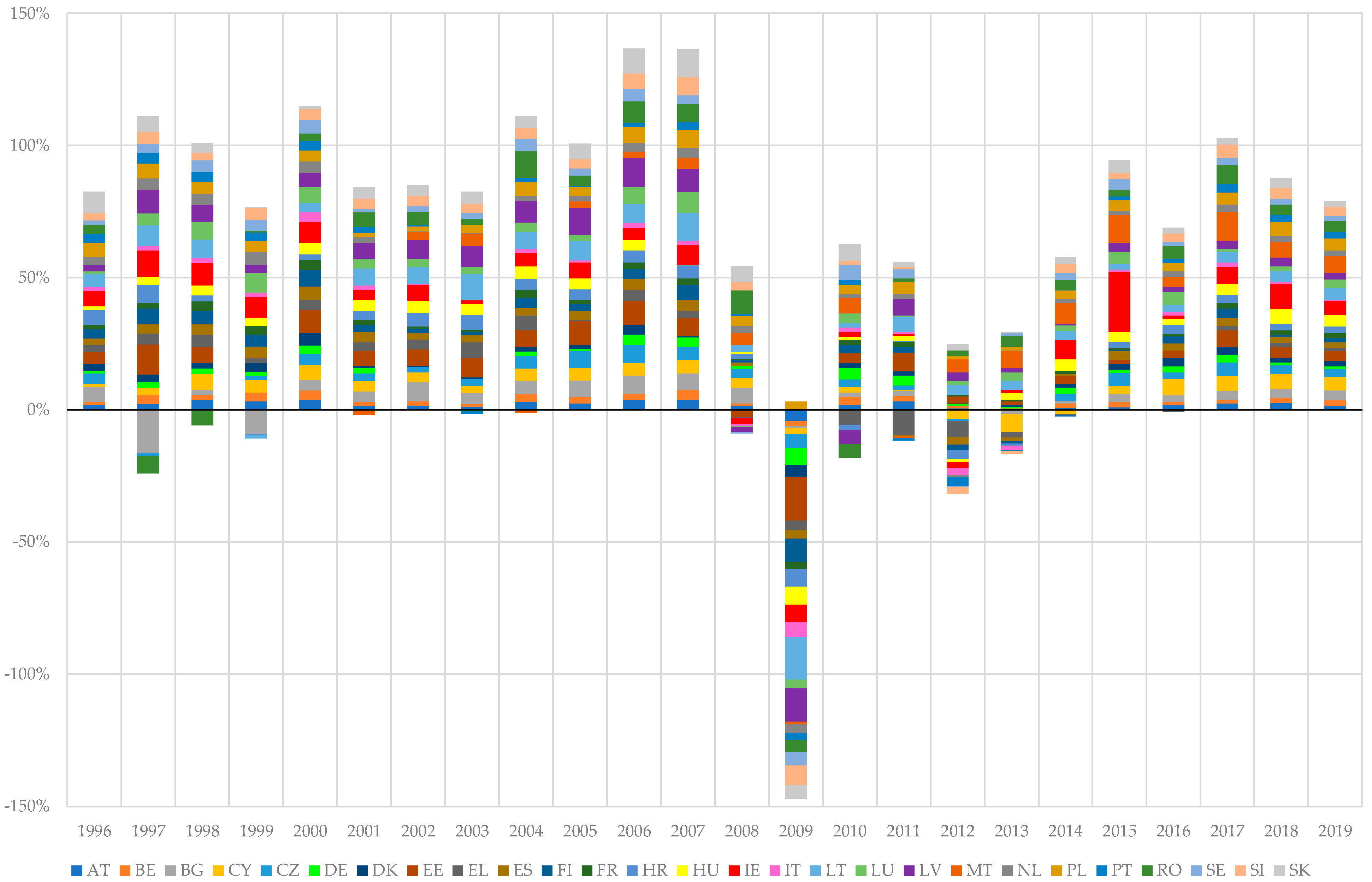However, the growth of European countries varies considerably [7,9,10,33,34]. In this regard, Figure 1 shows the added-value growth of European Union countries.

Although Europe has begun to emerge from the great global recession of 2008–2009, there are new concerns about whether it will be able to restore its long-term growth to pre-crisis rates, especially in the context of new international challenges [35,36], such as rising inflation (especially energy prices), increasing international-trade protectionism, problems in global supply chains, the effects of sanctions over the Ukrainian war, Brexit, etc. The average annual growth of the European Union before 2006 stood at 2.6%, while between 2007 and 2016 it fell to 0.9%.

Assessing the impact of the European integration process is a complex and long-term process. Traditional indicators such as GDP per capita do not allow us to analyze its full extent [21]. Productivity growth is recognized as a measure of an economy’s long-term growth potential. It is well documented that the loss of productivity in Europe since the mid-1990s led to a slowdown in growth and may reverse the effects of integration in the long run [14,15,18,20,24,37].

Under the neoclassical growth model, the output is measured on the basis of several growth-related inputs [1,2]. The growth accounting methodology also enables growth measurements in terms of the contributions of the components of productivity, i.e., labor, capital, and intermediate inputs to growth [12,14,18]. The labor input comprises changes in hours worked and in persons employed but also changes in the composition of employment in terms of age, gender, and educational qualifications over time. The capital input includes assets such as physical tools, plants, and equipment [20,21,38].

Figure 1. Added-value growth of European Union countries (1996–2019). Source: adapted from WIIW [39].

Figure 1. Added-value growth of European Union countries (1996–2019). Source: adapted from WIIW [39].

Numerous studies have used this approach to study productivity, especially since the 2000s. For instance, Bergeaud et al. [40] studied labor productivity trends (labor composition, total employment, and the average of hours worked) in 13 countries from the period of 1890–2012. The authors identified factors that at various times halted the convergence process, mainly due to financial crises and wars, which caused major jumps in the level of productivity.

Burda and Severgnigni [21], based on the growth accounting approach, analyzed labor and capital as factors of production in 30 European countries over the period of 1994–2004. Their findings show that the new members from Central and Eastern Europe benefited from an acceleration of productivity, while the other European countries suffered from a productivity slowdown.

Inklaar et al. [14] analyzed European growth compared to US growth between 1995 and 2015. Specifically, they measured the growth of technology and diverse types of capital and labor, as well as the inputs of energy, materials, and services for different industries. Their results showed that in both Europe and the US, information and communications technologies (ICTs) significantly contributed to productivity growth (although the trend in European industries revealed less ICT intensity).

Decomposing the sources of growth (capital, labor, and total factor productivity growth) for the joint EU27 shows both capital stock deceleration and how serious the effect of recession on the growth of the total hours worked in Europe was [14,24] (see Figure 2).

Productivity in the EU showed a declining trend up to 2006. At that time, several European countries introduced labor-market reforms to reintegrate the long-term unemployed and increase the participation rate, but the impact on the growth of productivity was temporary [14,18]. Nevertheless, since the great recession, the EU has experienced a sharp decline in labor-force participation and in the number of hours worked, which has not been offset by the substitution of capital with labor [15,24]. Indeed, capital inputs generally give a positive contribution to growth; however, it has been shown that they also slowed it down in the post-crisis period, reflecting the weak recovery of investment in the EU (perhaps due to the lack of investment in ICT-intensive industries [14]).

Figure 2. Contributions to value-added growth of EU27. Source: adapted from WIIW [39].

Figure 2. Contributions to value-added growth of EU27. Source: adapted from WIIW [39].

Overall, productivity growth is the weakest link in Europe’s growth. Even during the pre-crisis period, it had a declining trend in the European economy, and during the period of 2008–2010, it plummeted and barely recovered to a positive level (2%). The weak pace of productivity growth in Europe characterizes the slow diffusion of technology and innovation, largely related to other major productivity-related capital investments [14,15]. Although the general trends of productivity slowdown and recovery apply to most countries, there are significant differences among member countries.

Given these data and considering the above literature review on economic growth and productivity, in this paper, we attempt to answer four research questions, the first one of which being the following: (1) How does productivity contribute to the value-added growth of EMU or non-EMU countries?

Further, similarly to previous studies [7,10,14,15,21,22,23,40], we delve into the above question by decomposing productivity into the components of labor productivity and capital productivity. We thus pose the following research questions: (2) How does labor productivity contribute to the value-added growth of EMU or non-EMU countries?; and (3) How does capital productivity contribute to the value-added growth of EMU or non-EMU countries?

Finally, previous studies have indicated that the free movement of labor affects the composition of the European labor market; this may partly explain the performance of labor productivity [7,23,25,41].

In this sense, immigration allows an increase in labor-force participation to be obtained. In the case of workers with a high level of education, it leads to growth that is also transferred to neighboring countries, thus having a statistically significant impact not only on the growth of the country itself but also on that of neighboring countries in the same integration zone [7].

Moreover, the current low growth of productivity per worker and lower labor-force participation are associated with the aging population in European countries, which is likely to lead to lower productivity in the long run [23]

Hence, most countries have a strong interest in creating conditions to attract and retain local and foreign skilled labor and, consequently, in reinforcing the productivity gains needed to sustain economic growth [25].

This raises the last research question: (4) Do migrations have an impact on labor productivity in Europe? In other words, does the productivity of foreign workers contribute to the value-added growth of EMU or non-EMU countries?

3. Methodology

Productivity growth is an important indicator of an economy’s long-term growth potential [15]. In this regard, the EU-Klems database [20] decomposes the value-added growth into contributing factor inputs, mainly several types of labor and capital inputs. This approach allows researchers to assess the contribution of labor and capital to economic growth [18]. Moreover, EU-Klems has been developing productivity measures for the European Union since 1990, culminating in the publication of the first EU Productivity and Growth Database in 2008, with several key scientific publications and updates since then [15,18,21]. The latest release of productivity data provides a unique opportunity to analyze a large sample considering a long period [20]—in this case, productivity growth and the effects of the interactions among 22 European countries during the last decade of the 21st century.

Hence, value-added growth can be decomposed in different ways: (i) by considering the growth of capital stock, the average of hours worked, and employment; and (ii) by adding to the latter the change in labor composition or capital composition, with such indicators being defined as the change in labor or capital services minus the increase in the hours worked, respectively [20]. This approach allowed us to explain the growth of added value from three alternative perspectives depending on the explanatory variables considered: (1) overall productivity, (2) labor productivity, and (3) capital productivity. Further, given the freedom of movement of labor in the EU, we tested the influence of the growing migrant population on value-added growth. Thus, a fourth approach consists of replacing, in the first decomposition, the employment of the migrant population by level of attainment (basic, intermediate, and advanced).

3.1. Data

The data came from WIIW (Vienna Institute for International Economic Studies), the latest update of the Growth and Productivity database. This database is the successor of EU-Klems and provides a unique opportunity to analyze the data of the contributions to the growth of the added value and labor productivity of the EU27 member states. EU-Klems uses a growth accounting framework to decompose the growth of the aggregate added value into several contributions of labor and capital, i.e., labor quantity and quality, capital quantity and quality for the total economy and for manufacturing, and market services [20].

This allowed us to cover a lengthy period, two decades of the XXI century, and to analyze the interactions of a large set of economies (22 European countries after data harmonization) at the country level. Finally, it singled out the growth-contributing productivity components.

In addition, as the last research question focuses on foreign workers’ educational attainment, we also employed data from International Labor Organization Statistics (ILOSTAT) [42].

To harmonize the data from the WIIW and ILOSTAT databases and because of missing data of some countries, the period analyzed was finally selected as follows: In order to compare the results obtained, the period of 2009–2018 was selected for the first, second, and third research questions, and due to the singularity of the data, the period of 2005–2018 was selected for the fourth question.

For the same reasons mentioned above, the selected sample of European countries excludes five EU27 countries (Bulgaria, Croatia, Cyprus, Malta, and Romania). Currently, the remaining 22 countries (Euro: Austria, Belgium, Germany, Estonia, Greece, Spain, Finland, France, Ireland, Italy, Lithuania, Luxemburg, Latvia, Netherlands, Portugal, Slovenia, and Slovakia) account for nearly 90% of the European Union’s nominal GDP. In addition, the sample includes 5 countries (Non-Euro: Czechia, Denmark, Hungary, Poland, and Sweden) that are not members of the eurozone. Nevertheless, such countries have interacted intensively with the rest of the European countries for the last 15 years. This is remarkably interesting because it provided us the possibility to analyze the relationship between value-added growth and eurozone membership.

As is well known, the year of entry of each country analyzed into the eurozone depended on the degree of compliance with the criteria for accession to the monetary union, which was influenced by the national and international situations to which these countries were exposed. To take this into account, in the data panel used (for each variable, we work with a matrix of dimension countries x years), we introduced a dummy variable that takes the value of 1 for each of the years in which a country has belonged to the eurozone and 0 otherwise.

3.2. Models

The close interrelation among the countries of the European Union requires the consideration of the spatial spillover that exists among all of them. The growth of a country’s added value cannot be explained solely based on its performance, since the influence of its neighbors is relevant in terms of economic growth [3,5]. Therefore, to answer the research questions posed above, the statistical models needed to consider the spatial component.

The literature on spatial econometrics establishes a classification of models according to the importance of different spatial interactions [43]: (i) endogenous interaction—the economic decision of an agent or geographical zone depends on the decision of its neighbors; (ii) exogenous interaction—an agent’s economic decision depends on the observable characteristics of its neighbors; and (iii) a spatial correlation of the effects due to the same unobserved characteristics. In addition to these interactions, by introducing a panel data model, we could analyze the presence of random or fixed effects and, within these, spatial or temporal effects, or both [10,31,44]. Thus, the general nesting model is as follows:

$$\begin{gathered} ∆{\mathrm{lnY}}_{\mathrm{it}}={ \mathsf{\alpha }}_{\mathrm{t}}+{\mathsf{\mu }}_{\mathrm{i}}+\mathsf{\delta } \mathrm{W}∆{\mathrm{lnY}}_{\mathrm{it}}+{\mathsf{\beta }}_{\mathrm{n}}{\mathrm{X}}_{\mathrm{n},\mathrm{it}}+{\mathsf{\vartheta }}_{\mathrm{n}}{\mathrm{WX}}_{\mathrm{n},\mathrm{it}}+{\mathrm{u}}_{\mathrm{it}} \\ {\mathrm{u}}_{\mathrm{it}}={\mathsf{\lambda }\mathrm{Wu}}_{\mathrm{it}}+{\mathsf{\epsilon }}_{\mathrm{it}}, \end{gathered}$$

(1)

where $\mathrm{i}$ is an index for the cross-sectional dimension (eurozone countries NUTS-I); $\mathrm{t}$ is an index for the time dimension; $∆{\mathrm{lnY}}_{\mathrm{it}}$ is value-added growth in logs; $\mathrm{W}$ is the spatial weight matrix; $\mathrm{W}∆{\mathrm{lnY}}_{\mathrm{it}}$ is the spatial autoregressive component of value-added growth; ${\mathrm{X}}_{\mathrm{n},\mathrm{it}}$ is a matrix of n explanatory variables at time $\mathrm{t}$; ${\mathrm{WX}}_{\mathrm{n},\mathrm{it}}$ is the spatial interaction of n explanatory variables of different regional units; ${\mathsf{\alpha }}_{\mathrm{t}}$ and ${\mathsf{\mu }}_{\mathrm{i}}$ are the vectors of time-period effects and spatial fixed effects, respectively; δ is the spatial autoregressive coefficient; ${\mathsf{\beta }}_{\mathrm{n}}$ and ${\mathsf{\vartheta }}_{\mathrm{n}}$ are the vectors of n parameters to be estimated; and $\mathsf{\lambda }$, ${\mathrm{Wu}}_{\mathrm{it}}$, and ${\mathsf{\epsilon }}_{\mathrm{it}}$ are the spatial autocorrelation coefficient, the interaction effects among the disturbance terms of the different regional units, and the vectors of the disturbance terms, respectively.

Since we intend to consider the impact on the value-added growth of the European area members, we proposed a two-regime spatial model. For this purpose, we followed the methodology proposed by Elhorst and Freret [45] to test for a political yardstick competition in France.

In our case, we modified this model to incorporate additional modeling estimation, different fixed effects, and the corresponding ratio test to select the best model (see Appendix A for additional details). The regime variable included in the model allowed us to analyze if the value-added growth for a country is sensitive to changes in the economic situation in neighboring countries when belonging to the European area.

We estimated the impact exerted on the value-added growth by different variables related to capital productivity and labor productivity, and the models to estimate were different depending on the explanatory variables:

• Model 1—overall productivity—considers the growth of capital stock (K), the average hours worked (AHW), and employment (E);
• Model 2—labor productivity—considers the growth of labor composition (LC), employment (E), and the average hours worked (AHW);
• Model 3—capital productivity—considers the growth of capital composition (KC), employment (E), and the average hours worked (AHW);
• Model 4—the effect of foreign workers—considers the growth of capital stock (K), the average hours worked (AHW), and the value of participation rate of foreign-born working-age population on the total working-age population by level of educational attainment (basic, intermediate, and advanced).

The general versions of the SDM and SAR models can be seen in Equations (A1) and (A2), respectively (Appendix A). For each modeling, we used four models, resulting in eight models to be estimated (see Equations (A3)–(A10) in Appendix B). In the following section, we estimate these equations to select those that present the best fit for each of the study goals and, consequently, to improve our understanding of the factors underlying value-added growth and the role played by membership or non-membership in the eurozone.

4. Results

After defining the models, the next step before their estimation was the selection of the spatial weight matrix with the best performing among Equations (A3)–(A6). This is a relevant matter because it reflects the neighborhood structure for each country and thus the spatial influence exerted or received by other neighboring countries. For this purpose, we considered several specifications based on geographic distance, namely, k-nearest neighbors (k = 1 to 10), the distance between the centroids of the various regions from minimum to maximum and with cut-off kilometers for intermediate distances, and inverse distance matrices with a distance decay factor whose off-diagonal elements are defined by w_ij = 1/d_ijα, where α = 1.00, 1.50, … and 3.00. After estimating the SDM models for the latter specifications, we focused on the log-likelihood ratio and the value of the residual variance. The estimates of the models with higher log-likelihood and lower residual variance are the best-performing ones. In our case, whatever the estimated model, the selected spatial weight matrix was a normalized row of the two nearest neighbors. Regardless of these results, it is reasonable to assume that economic growth is influenced by the situation in the nearest neighboring countries.

To determine whether space and time are significant, we performed the likelihood ratio test for the four models, both SDM and SAR models (see

Table 1. Likelihood ratio test for significance of spatial and/or time-period fixed effects.

Fixed Effect	Model 1	Model 2	Model 3	Model 4
SDM
Spatial	36.2631, 22, 0.0285	68.3139, 22, 0.0000	73.4619, 22, 0.0000	33.6999, 22, 0.0527
Time-period	37.8668, 10, 0.0000	26.9236, 10, 0.0027	31.1518, 10, 0.0006	60.5180, 14, 0.0000
SAR
Spatial	39.2841, 22, 0.0131	70.2778, 22, 0.0000	69.6843, 22, 0.0000	44.0943, 22, 0.0035
Time-period	38.3994, 10, 0.0000	31.5482, 10, 0.0005	33.8633, 10, 0.0002	60.9845, 14, 0.0000

Note: LR test, degrees of freedom, and probability. The null hypothesis is that the fixed effects are not jointly significant. When the p-value is less than 0.01 the null hypothesis must be rejected, otherwise, it cannot be rejected (in bold).

). The results indicate that we cannot reject the null hypothesis that spatial fixed effects are not significant for models 1 (SDM and SAR) and 4 (SDM). Instead, for the rest of the models, we rejected the null hypothesis for both fixed effects; therefore, a two-way fixed effects model needed to be applied.

Having selected the fixed effects that work in our models, the next step was to analyze whether the SDM can be simplified to SAR [46]. To do this, we calculated the likelihood ratio (LR) test for SDM versus SAR, so that when its likelihood was less than 0.05, it implied that the SDM cannot be simplified to SAR. The results for the different models were as follows:

• For Models 1 to 3, the LR test was higher than 0.05, and we could not reject the null hypothesis that ϑ = 0, for which the models can be simplified to SAR. The models to estimate were SAR models with spatial and time-period fixed effects for Models 2 and 3 and only with the latter for Model 1;
• For Model 4, as the LR test was lower than 0.05, we could reject the hypothesis that ϑ = 0, and the model could not be simplified to SAR, which implies that spatially lagged independent variables are significant. The model to be estimated was the SDM with time-period fixed effects.

In short, the models to be estimated are the following:

• Model 1, overall productivity (SAR with time-period fixed effects):

$$\begin{gathered} ∆{\mathrm{lnY}}_{\mathrm{it}}={\mathsf{\alpha }}_{\mathrm{t}}+{\mathsf{\delta }}_1{\mathrm{d}}_{\mathrm{it}}\mathrm{W}∆{\mathrm{lnY}}_{\mathrm{it}}+{\mathsf{\delta }}_2\left(1-{\mathrm{d}}_{\mathrm{it}}\right)\mathrm{W}∆{\mathrm{lnY}}_{\mathrm{it}}+ \\ {\mathsf{\beta }}_1∆{\mathrm{lnK}}_{\mathrm{it}}+{\mathsf{\beta }}_2∆{\mathrm{lnE}}_{\mathrm{it}}+{\mathsf{\beta }}_3∆{\mathrm{lnAHW}}_{\mathrm{it}}+{\mathrm{u}}_{\mathrm{it}} \end{gathered}$$

(2)

• Model 2, labor productivity (SAR with spatial and time-period fixed effects):

$$\begin{gathered} ∆{\mathrm{lnY}}_{\mathrm{it}}={\mathsf{\alpha }}_{\mathrm{t}}+{\mathsf{\mu }}_{\mathrm{i}}+{\mathsf{\delta }}_1{\mathrm{d}}_{\mathrm{it}}\mathrm{W}∆{\mathrm{lnY}}_{\mathrm{it}}+{\mathsf{\delta }}_2\left(1-{\mathrm{d}}_{\mathrm{it}}\right)\mathrm{W}∆{\mathrm{lnY}}_{\mathrm{it}}+ \\ {\mathsf{\beta }}_1∆{\mathrm{lnLC}}_{\mathrm{it}}+{\mathsf{\beta }}_2∆{\mathrm{lnE}}_{\mathrm{it}}+{\mathsf{\beta }}_3{\mathrm{AHW}}_{\mathrm{it}}+{\mathrm{u}}_{\mathrm{it}} \end{gathered}$$

(3)

• Model 3, capital productivity (SAR with spatial and time-period fixed effects):

$$\begin{gathered} ∆{\mathrm{lnY}}_{\mathrm{it}}={\mathsf{\alpha }}_{\mathrm{t}}+{\mathsf{\mu }}_{\mathrm{i}}+{\mathsf{\delta }}_1{\mathrm{d}}_{\mathrm{it}}\mathrm{W}∆{\mathrm{lnY}}_{\mathrm{it}}+{\mathsf{\delta }}_2\left(1-{\mathrm{d}}_{\mathrm{it}}\right)\mathrm{W}∆{\mathrm{lnY}}_{\mathrm{it}}+ \\ {\mathsf{\beta }}_1∆{\mathrm{lnKC}}_{\mathrm{it}}+{\mathsf{\beta }}_2∆{\mathrm{lnE}}_{\mathrm{it}}+{\mathsf{\beta }}_3∆{\mathrm{lnAHW}}_{\mathrm{it}}+{\mathrm{u}}_{\mathrm{it}} \end{gathered}$$

(4)

• Model 4, the effect of foreign workers (SDM with time-period fixed effects):

$$\begin{gathered} ∆{\mathrm{lnY}}_{\mathrm{it}}={\mathsf{\alpha }}_{\mathrm{t}}+{\mathsf{\delta }}_1{\mathrm{d}}_{\mathrm{it}}\mathrm{W}∆{\mathrm{lnY}}_{\mathrm{it}}+{\mathsf{\delta }}_2\left(1-{\mathrm{d}}_{\mathrm{it}}\right)\mathrm{W}∆{\mathrm{lnY}}_{\mathrm{it}}+{\mathsf{\beta }}_1∆{\mathrm{lnK}}_{\mathrm{it}}+{\mathsf{\vartheta }}_1\mathrm{W}∆{\mathrm{lnK}}_{\mathrm{it}}+ \\ {\mathsf{\beta }}_2∆{\mathrm{lnAHW}}_{\mathrm{it}}+{\mathsf{\vartheta }}_2\mathrm{W}∆{\mathrm{lnAHW}}_{\mathrm{it}}+{\mathsf{\beta }}_3{\mathrm{lnBasic}}_{\mathrm{it}}+{\mathsf{\vartheta }}_3{\mathrm{WlnBasic}}_{\mathrm{it}}+{\mathsf{\beta }}_4{\mathrm{lnIntermediate}}_{\mathrm{it}}+ \\ {\mathsf{\vartheta }}_4{\mathrm{WlnIntermediate}}_{\mathrm{it}}+{\mathsf{\beta }}_5{\mathrm{lnAdvanced}}_{\mathrm{it}}+{\mathsf{\vartheta }}_5{\mathrm{WlnAdvanced}}_{\mathrm{it}}+{\mathrm{u}}_{\mathrm{it}} \end{gathered}$$

(5)

All four models were estimated using maximum likelihood because the panel data models include spatial and/or temporal fixed effects (see

Table 2. Two-regime spatial-model estimation for value-added growth.

Determinant	Model 1 SAR (Time-Period Fixed Effects)	Model 2 SAR (Spatial and Time-Period Fixed Effects	Model 3 SAR (Spatial and Time-Period Fixed Effects)	Model 4 SDM (Time-Period Fixed Effects)
$∆\mathrm{lnK}$	0.947 *** (12.683)			0.946 *** (12.324)
$∆\mathrm{lnLC}$		−0.345 (−1.068)
$∆\mathrm{lnKC}$			−1.003 *** (−9.173)
$∆\mathrm{lnE}$	0.814 *** (7.216)	1.016 *** (6.642)	1.017 *** (8.388)
$∆\mathrm{lnAHW}$	0.431 ** (1.996)	0.647 *** (2.577)	0.456 ** (2.126)	0.556 *** (3.088)
$\mathrm{lnBasic}$				−0.716 *** (−4.331)
$\mathrm{lnIntermediate}$				−11.79 *** (−2.844)
$\mathrm{lnAdvanced}$				8.859 ** (2.197)
$\mathrm{W}∆\mathrm{lnK}$				0.791 *** (3.037)
$\mathrm{W}∆\mathrm{lnAHW}$				0.260 (0.914)
$\mathrm{WlnBasic}$				0.625 *** (3.868)
$\mathrm{WlnIntermediate}$				1.145 (0.235)
$\mathrm{WlnAdvanced}$				2.020 (0.431)
Reg. 1 (dum. 1)	0.508 *** (5.273)	0.437 *** (4.015)	0.486 *** (4.853)	0.532 *** (7.072)
Reg. 2 (dum. 0)	0.119 * (1.808)	0.073 (1.003)	0.125 * (1.821)	0.497 (0.619)
R2	0.802	0.750	0.819	0.774
Adjusted R2	0.788	0.701	0.784	0.753
Residual var.	2.821	3.561	2.578	3.171
Log-likelihood	−428.141	−452.941	−418.23	−617.701
Observations	220	220	220	308

Note: T-statistics are shown in parentheses. Statistical significance: * 10% level, ** 5% level, *** 1% level.

). We used a balanced panel dataset of 22 European countries for the periods of 2009–2018 (Models 1, 2, and 3), and 2005–2018 (Model 4). As mentioned above, the four models aim to analyze the explanatory value of productivity-related variables on value-added growth. These models focus on the growth rates of the capital stock and labor inputs (Model 1), changes in labor composition (Model 2), changes in capital composition (Model 3), and changes in capital stock, hours worked, and the participation rate of the foreign-born working-age population by educational attainment (Model 4).

4.1. Model 1: Impact of Changes in Capital Stock and Labor Inputs on Added Value

All independent variables were significant at the 1% level (except for AHW, at the 5% level). The coefficients were positive, indicating the direct relationship between the growth of added value and those of capital stock, employment, and the average of hours worked. Their values were remarkably similar (between 0.8 and 0.9), except for the growth of the average of hours worked, which seemed to exert a smaller influence on the growth of added value.

Regarding the estimated coefficients for the two regimes, it was observed that, for the first regime (when the dummy variable is 1, ${\mathrm{d}}_{\mathrm{it}}$ = 1), the coefficient was positive and significant at the 1% level. This means that the value-added growth of a country is related to the economic growth of its neighbors when they belong to the eurozone. In contrast, when the dummy variable was 0 (the country does not belong to the eurozone), the coefficient was significant at the 10% level, but with a smaller effect than the previous case. As Table 2 shows, the value of the coefficient when belonging to the eurozone is much bigger than that of the second regime. This tresses the relevance of the carry-over effects of neighbors’ growth in the first regime.

4.2. Model 2: Impact of Changes in Labor Composition on Added Value

This model is similar to the latter after incorporating labor composition instead of capital stock growth. Labor composition can be defined as the difference between labor-service growth and hours-worked growth [20]. After estimating, we could observe that this new variable was not significant; therefore, the goodness of fit was worse. The remaining independent variables (employment and the average of hours worked) were significant, even with larger coefficients than those for Model 1. The removal of capital stock growth of Model 1 and its replacement with labor composition led to an increase in the coefficients.

Similar to the above-mentioned Model 1, the spatially lagged dependent variable was positive and significant at the 1% level, and its coefficient’s value was less than twice the value for Model 1, which highlights the combined effect of capital-service growth and the membership of the eurozone. Unlike the case of Model 1, when the country did not belong to the euro area, the estimation of the second regime (${\mathrm{d}}_{\mathrm{it}}$ = 0) was not significant.

4.3. Model 3: Impact of Changes in Capital Composition on Added Value

This model is similar to the above but replaces labor composition with capital composition, which can be defined as the capital-service growth minus the capital stock growth [20]. As can be seen in Table 2, employment and hours-worked growth are significant with a positive sign, with the estimated coefficient being similar to that of Model 2.

In this sense, it is important to highlight the negative sign of the estimated coefficients for the growth of capital composition, which could be interpreted as the negative impact on a country’s economic growth when capital services grow above capital stock, that is, when capital composition is positive. However, this value is offset by the increase in the coefficients of employment and of the average of hours worked.

As for the two regimes, the situation is analogous to that of Model 2, differing only in the values of their coefficients (slightly higher) and in the significance at the 10% level of the estimated coefficient when a country does not belong to the eurozone. Although the economic growth of neighboring countries belonging to the eurozone remains more relevant, when considering the growth of capital services rather than the growth of labor services, the effect seemed to be mitigated, due to the higher levels of capitalization of the euro area member states.

4.4. Model 4: Impact of Changes in Capital Stock, Hours Worked, and Foreign-Born Working Population by Level of Education Attainment on Value-Added Growth

The main difference between Model 1 and Model 4 is the substitution of employment growth with the participation rate of the foreign-born working-age population by educational attainment. It is not surprising, therefore, that the values and significance of the common variables are similar. Thus, we focused on the impact of the foreign-born population on economic growth. In this regard, the most outstanding results were the significance at the 1% level and the negative sign of the estimated coefficient for the foreign-born population with basic and intermediate education levels. The negative signs of these coefficients implied an inverse relationship between the participation rate of the foreign-born population with lower educational levels and value-added growth. When the origin of migration corresponds with non-European countries, the obvious consequence of this finding is that, in those countries with higher illegal immigration or less selective immigration policies, regardless of characteristics such as the educational level, the impact on economic growth would be negative. The potential of these foreign workers to meet the needs of the labor market would not be exploited.

There is no doubt that there is a direct relationship between the educational level and the contribution to value-added growth, reinforcing the productivity gains needed to sustain economic growth [25]. In the case of skilled workers, they also tend to generate business opportunities with their countries of origin [7,25]. However, it is also common for immigrants with low levels of education to occupy low-skilled and low-paid jobs, precisely those that the native population is more reluctant to fill and whose contribution to productivity growth is more limited. These populations are greater than the foreign-born population with advanced education, and their negative coefficients are jointly larger than the positive one for advanced education (also significant at the 5% level).

Regarding the spatially lagged independent variables, we observed the positive sign and significance at the 1% level of capital stock growth. This is the consequence of increasing the returns of scale in capital accumulation in neighboring countries, which are extended to the country itself, demonstrating the synergies and positive externalities derived from capital accumulation processes. An analogous situation could be observed regarding the coefficient for the rate of foreign-born working-age participation with a basic educational level, which is particularly conspicuous because the negative sign of the same variable is not spatially lagged.

When we introduced in the model the educational attainment level, the significance of the estimated coefficients for the regimes was similar to that found in Model 2. The economic growth of a country is impelled by those of the neighboring countries when they are members of the eurozone. Nevertheless, in this case, the estimated coefficient was greater than that for Model 2, which implies that the foreign-born population increases the impact of the spatially lagged dependent variable.

4.5. Direct, Indirect, and Total Effects of Estimated Models

The SAR and SDM estimated models capture both the direct effect of neighbors’ expected outcomes on a country’s outcomes and the indirect (or spillovers) impact on other European countries. For correctly measuring the effect of the productivity variables on value-added growth, it was necessary to analyze the spatial spillovers based on three types of effects [46]: (i) direct, which summarizes the impact of changes in each explanatory variable in country i on the value-added growth of the same country; (ii) indirect, reflecting the impact of the changes in independent variables of neighboring countries on the growth of a country; and (iii) total, which is a scalar summary measure that includes both direct and indirect effects and can be interpreted as the total impact on the dependent variable of the changes in an independent variable.

Regarding the estimated effects for Models 1 to 3 (see

Table 3. Direct, indirect, and total effects of the estimated models.

Model	Determinants	Direct Effects	Indirect Effects	Total Effects
Overall productivity (1)	$∆\mathrm{lnK}$	0.970 *** (11.968)	0.294 *** (3.628)	1.264 *** (9.182)
	$∆\mathrm{lnE}$	0.960 *** (8.190)	0.289 *** (3.762)	1.248 *** (7.794)
	$∆\mathrm{lnAHW}$	0.566 ** (2.533)	0.171 * (2.053)	0.738 ** (2.488)
Labor productivity (2)	$∆\mathrm{lnLC}$	−0.354 (−0.986)	−0.101 (−0.897)	−0.455 (−0.979)
	$∆\mathrm{lnE}$	1.163 *** (6.852)	0.322 *** (3.131)	1.485 *** (6.602)
	$∆\mathrm{lnAHW}$	0.764 ** (2.727)	0.213 * (2.021)	0.977 ** (2.663)
Capital productivity (3)	$∆\mathrm{lnKC}$	−1.034 *** (−8.398)	−0.376 *** (−3.503)	−1.410 *** (−6.957)
	$∆\mathrm{lnE}$	1.176 *** (9.107)	0.425 *** (3.924)	1.600 *** (8.309)
	$∆\mathrm{lnAHW}$	0.564 ** (2.318)	0.205 * (1.936)	0.769 ** (2.268)
The effects of foreign workers (4)	$∆\mathrm{lnK}$	1.084 *** (12.108)	1.425 *** (4.647)	2.509 *** (7.216)
	$∆\mathrm{lnAHW}$	0.665 *** (3.415)	0.738 * (2.031)	1.403 *** (2.983)
	$\mathrm{lnBasic}$	−0.612 *** (−3.506)	0.642 *** (3.489)	0.030 (0.145)
	$\mathrm{lnIntermediate}$	−10.389 ** (−2.360)	0.277 (0.046)	−10.112 (−1.418)
	$\mathrm{lnAdvanced}$	8.516 * (2.007)	3.389 (0.583)	11.905 * (1.718)

Note: T-statistics are shown in parentheses. Statistical significance: * 10% level, ** 5% level, *** 1% level.

), it is worth noting the significance of employment, capital stock, and capital composition at the 1% level, regardless of the effect considered, but with different signs, i.e., positive for the first two and negative for the latter. At the opposite end, we found the labor composition, which was not significant in any case. In all cases, the values of the direct effects are greater than those of the indirect effects, which points to the lesser importance exerted by the evolution of independent variables of neighboring countries on value-added growth. For the remaining variable (the average of hours worked), the significance, sign, and magnitude of the estimated coefficients were similar in the first three models, but unlike the previous variables, the direct and total effects were significant at the 5% level and at the 10% level for indirect effects. That is, neighboring countries seemed to exert a lesser influence on value-added growth.

Regarding Model 4, the above comments are applicable to this model for capital stock and the average of hours worked, making it more interesting to focus on the participation rate of the foreign-born working-age population on the total working-age population by level of educational attainment (basic, intermediate, and advanced). In this regard, it can be observed that only the total effect is significant at the 10% level for the advanced educational attainment ratio; the fact that it has positive sign points to a direct relationship between this ratio and value-added growth. For the working-age population with basic and intermediate educational levels, its lack of significance was due to the behavior of indirect effects, and their signs or significances compensate for the negative and significant direct effects.

5. Discussion

Since the introduction of the euro currency in the EU, the Monetary Union membership clearly became an instrument to support not only nominal convergence but also real convergence (employment, per capita income, etc.) [36,47].

Various studies have analyzed the effects of the eurozone membership on economic growth [1,2,8,9,21,27]. In this research study, we analyzed this relationship using the latest data by incorporating spatial patterns and interactions among European countries and considering the role played by factor endowments, both the capital stock and labor inputs through different indicators. We confirmed the results from previous studies that highlighted the relevance of productivity as an indicator of sustainable long-term growth [14,15,21,40].

Although the underlying reasons for not belonging to the eurozone differed from country to country (i.e., one cannot compare Denmark to Poland), in this study, we showed that the eurozone membership results in a direct relationship between a country’s economic growth and the growth of neighboring countries.

These findings are here observed in the different models developed to explain the effects on the growth of eurozone countries from the point of view of productivity components.

The same is true for non-members of the eurozone, but to a lesser extent (Model 1).

This can be due to several reasons: (i) In general (except for the Danish case), the non-Euro countries analyzed have a lower GDP; therefore, they more easily grow at higher rates, which is consistent with the convergence process observed in the EU. (ii) EU countries want to enter the Eurozone, although the common currency requires time (a long but inevitable journey of fiscal consolidation, the momentum for structural reforms in the market, sectors, and institutions, etc.). The significance of employment and hours-worked growth is especially noteworthy, which must not be surprising because of the importance of the service sector in European economies and thus its direct relationship with economic growth. In contrast, the spatial lag of hours worked is not significant (Model 4).

These findings are in line with Barro’s work and the standard neoclassical model [5,26]. Moreover, our findings add evidence to previous studies that analyzed the effects of the European integration process according to different socioeconomic drivers [1,3,6,16]. Furthermore, in our case, we added the components of productivity by exploiting the advantages of the use of spatial models to analyze cross-country interactions. In this sense, our work also extends the results obtained by Dreyer and Schmid [2], confirming the impact on the growth of eurozone member countries during the great economic recession and the following years.

Regarding the capital stock growth, we can observe the positive sign and significance at the 1% level. This is the consequence of increasing the returns to scale in capital accumulation both in the country and in neighboring countries, which spills over to nearby countries and demonstrates the synergies and positive externalities arising from the processes of capital accumulation. Thus, the importance of having a developed industrial sector or, in general, of maintaining a sustained increase in capital stock over time is underscored by the fact that it makes the country less dependent on the capitalization process of neighboring countries.

Regarding Model 2, in light of the results, we can say that neighboring Eurozone countries generate spatial spillovers that link their economic cycles. The eurozone’s growth effects are significant, so the euro-neighbors’ evolution influences the rest of the members in the same direction. However, in line with previous works [1,2,3], there is no evidence of a similar association in the case of non-Euro countries. This would highlight the relevance of the interactions among eurozone countries for economic growth.

As indicated above, there are concerns about whether European countries will be able to restore their pre-crisis growth rates. The prolonged productivity decline limits the positive contribution of capital inputs to growth. As Model 3 results show, in the case of the eurozone, this value is offset by employment and to a lesser extent by the increase in hours worked. Thus, it is necessary to establish a successful supply side policy in order to recover the role of capital accumulation, which is relative weak in the European Union. In addition, van Ark and Jäger [15] showed that labor policies focused on increasing the participation rate had temporary but positive effects on growth.

In fact, it is not possible to dissociate the processes of capital accumulation from the labor force. In this sense, immigration leads to an increase in labor-force participation. However, as our results reveal for Model 4, its impact on economic growth is different depending on the educational level of foreign workers.

In general, immigrants with low levels of education tend to occupy low-skilled and low-paid jobs, precisely those that the native-born population is more reluctant to fill and whose contribution to productivity growth is more limited. Therefore, it is not surprising to observe that the coefficients are negative for the foreign-born working-age population with basic and intermediate educational levels, while they are positive for those with an advanced educational level.

Therefore, it seems appropriate to point out that the use of selective migration policies according to educational attainment in combination with labor-market policies aimed at increasing the labor force could have a positive impact on the attraction and retention of international talent and thus on long-term growth.

In contrast, when we focus on the spatial lag of these variables, the positive sign for the basic educational level is particularly noteworthy. This could be explained by the labor-market segmentation at the European level and by the different immigration policies applied in neighboring countries. This could lead to the crowding out of foreign workers from countries with higher restrictive immigration policies than their neighbors.

In conclusion, to answer the research questions reported at the beginning of this paper, firstly, our results confirm that productivity gaps have significant effects on the growth of European countries, with these effects being most strongly spread among eurozone members, though they also affect other European countries, albeit to a lesser extent. Moreover, these effects are statistically significant during the period analyzed, which corresponds to the Great Recession and the immediate post-recession years.

Secondly, the decrease in productivity affects growth and economic recovery. In the case of Eurozone countries, the level of employment emerges as the main driver. Third, the slower accumulation of capital does not offset the decrease in employment levels either.

Fourth, regarding the contribution of foreign workers to the growth of euro countries, its impact varies according to the educational level of the foreign workers. Its influence is positive for other Eurozone countries in the case of skilled workers and negative for workers with basic and intermediate education levels. In the case of non-European countries, no significant evidence was found.

Finally, as a future research line, considering the availability of data, we propose to extend this research study to differences in productivity by individual European industries and, given their importance for innovation, to ICT (software, hardware and communication) asset-based industries.