
Targeting Sustainable Transportation Development: The Support Vector Machine and the Bayesian Optimization Algorithm for Classifying Household Vehicle Ownership


Abstract
:1. Introduction
2. Literature Review
2.1. Factors Influencing HVO
2.2. Methods Used for HVO Prediction

| Study | Study Aim | Model(s) Used | Hyperparameter Optimization |
|---|---|---|---|
| Chaipanha and Kaewwichian [47] | To provide a way for balancing the data using over- and under-sampling strategies. | kNN, NB, DTs | No |
| Manjushree, GH, Swamy and Giridharan [6] | To apply ML models to forecast the household characteristics that influence car ownership. | DTs, RF, MNL | No |
| Shao et al. [48] | To evaluate the nonlinear and interaction impacts of the built environment and motorcycles/E-bikes on automobile ownership using GBDT. | GBDT | Grid search |
| Pineda-Jaramillo [46] | To investigate the major factors that impact travel behavior among persons with restricted mobility to promote autonomous, healthy lives and healthy active transport modalities. | NB, kNN, DTs, SVM, RF, AdaBoost, NN, GBDT, CatBoost | Random search |
| Kaewwichian [14] | To remedy the imbalanced data problem in automobile ownership datasets. | DT, kNN, NB | No |
| Abdul Muhsin Zambang, Jiang and Wahab [42] | To approximate automobile ownership in Greater Tamale. | SGD, SVM, DT, RF, NB, kNN, | No |
| Wang et al. [49] | To anticipate ownership of electric vehicles. | AdaBoost | No |
| Sabouri, Brewer and Ewing [36] | To investigate the association between ride-sourcing services and household vehicle ownership. | DT, RF | No |
| Basu and Ferreira [41] | Through a comparison of econometric and machine learning models, to comprehend household automobile ownership in Singapore. | DT, RF, NN, SVM, LR, SGD, OLC | Grid search |
| Ha, Asada and Arimura [43] | To identify the variables that affect household car ownership trends in Phnom Penh. | RF, NN, MNL | No |
| Tanwanichkul et al. [50] | To approximate automobile ownership using ML methods. | DT, NN, MNL | No |
3. Research Motivations and Aims
4. Methodology
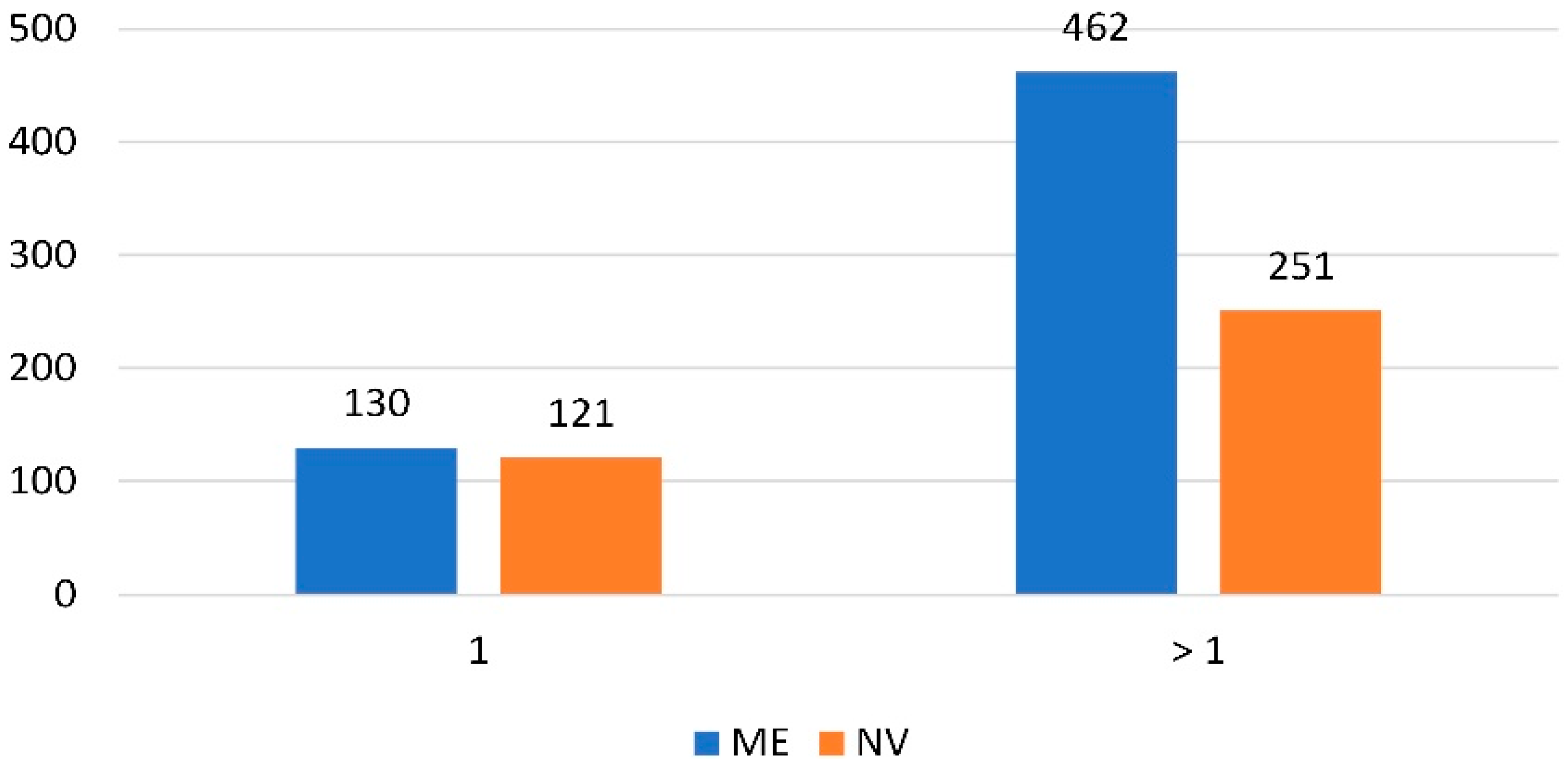
4.1. Data
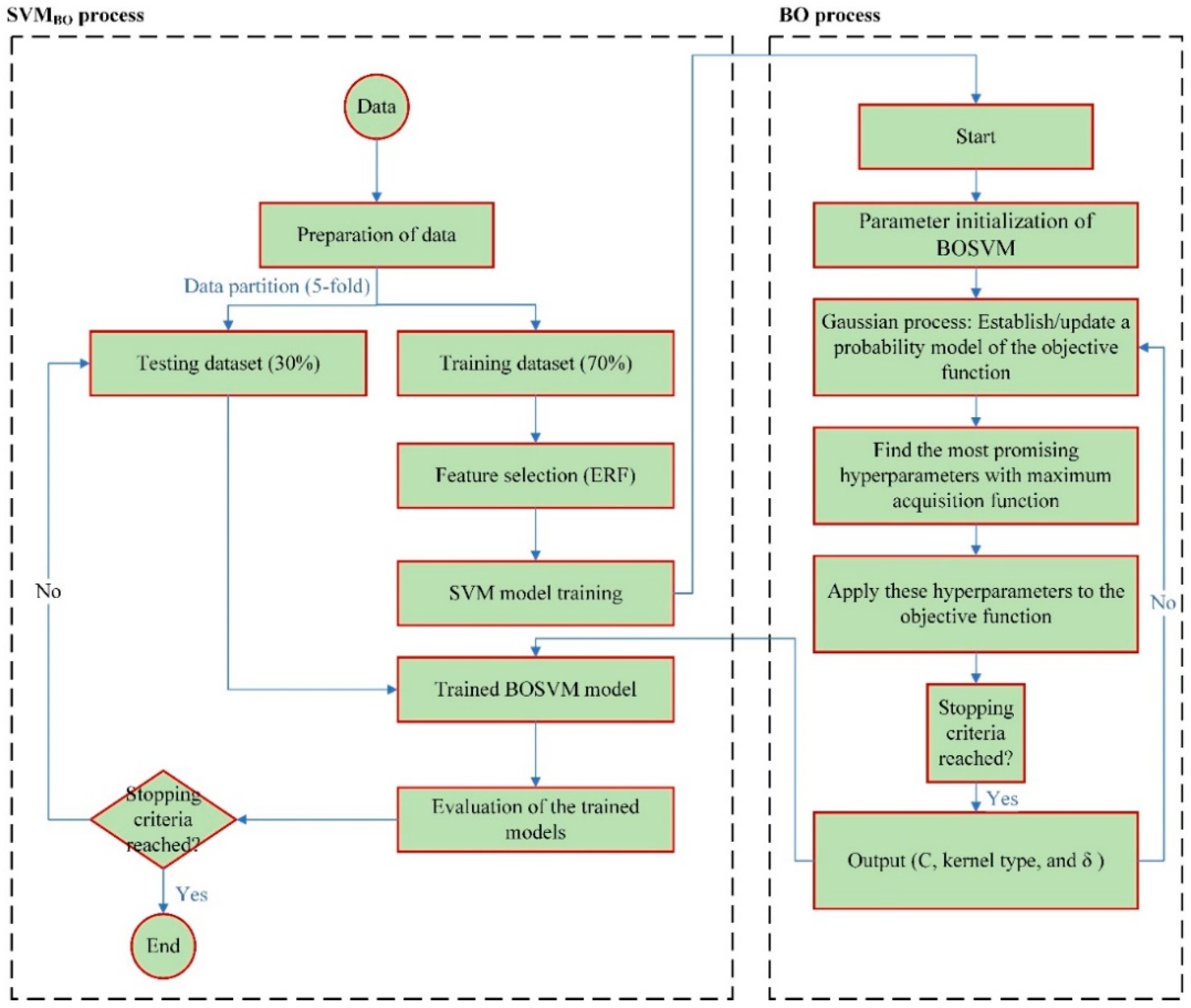
4.2. Support Vector Machines (SVM) and Bayesian Optimization (BO) Algorithm
4.3. Models’ Performance Assessment
5. Results
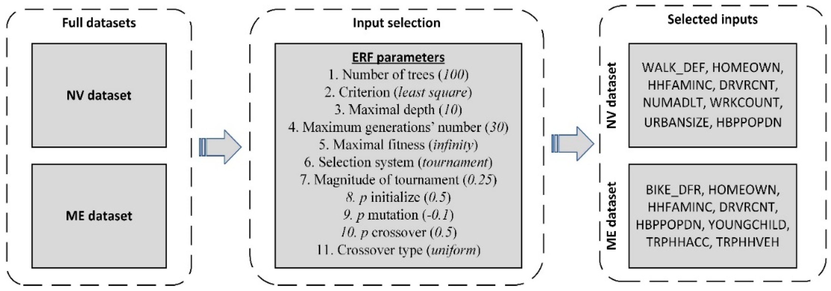
5.1. Input Selection
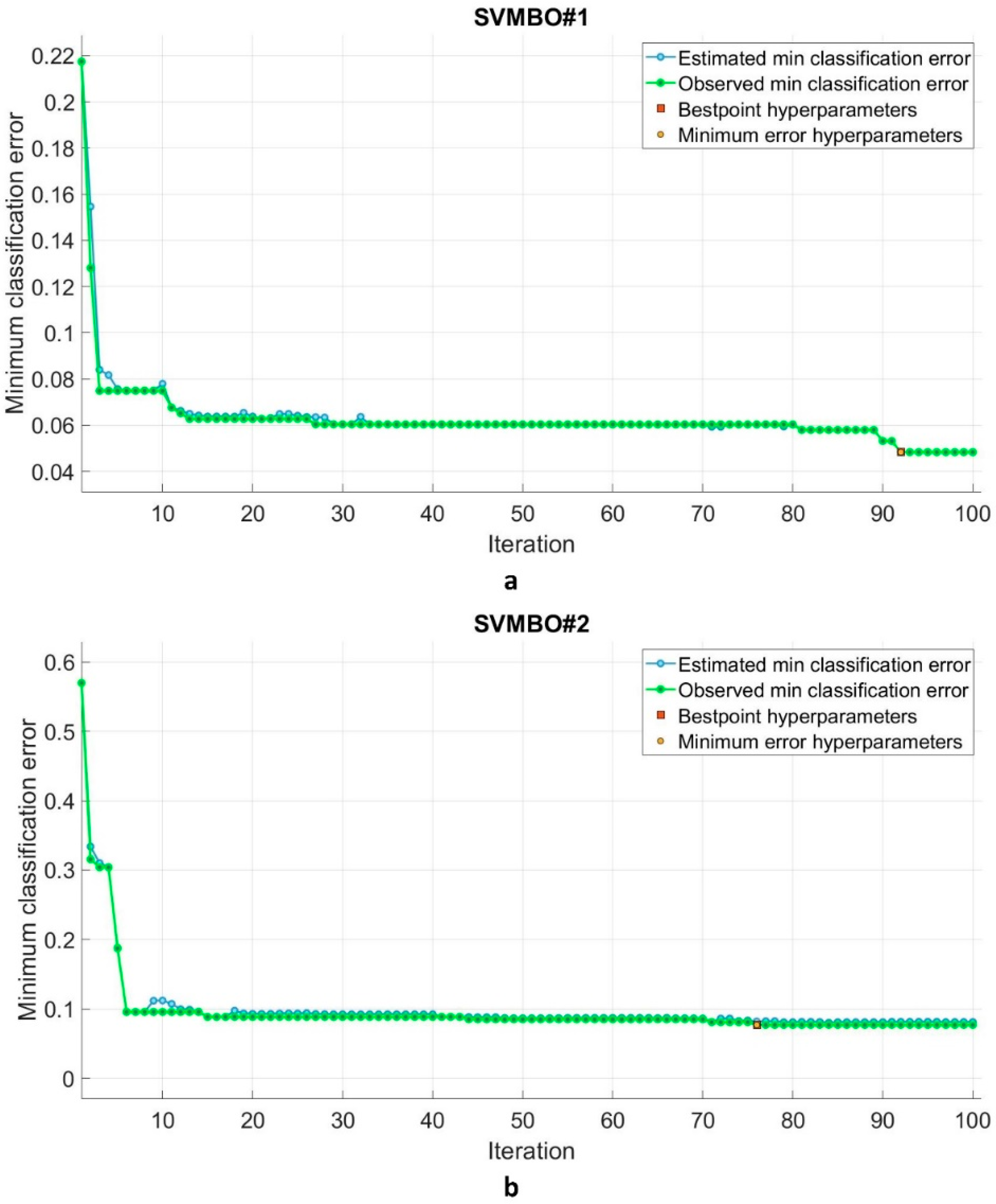
5.2. SVM and SVMBO Models’ Development and Assessment
- Processing and preparing data: randomly dividing the dataset into a training set and a testing set with an appropriate ratio (70:30).
- Assessment of fitness: before optimizing the target parameter value, estimate, and assess the fitness function.
- Adjustment of parameters: update the optimization criteria satisfied by the parameters based on every iteration’s finding.
- Halt condition inspection: once the optimization stop condition is fulfilled, the optimal parameters are determined.
6. Discussions
Implications for Academic and Policy-Making
7. Conclusions
- These two models took 375.55 s on average to train.
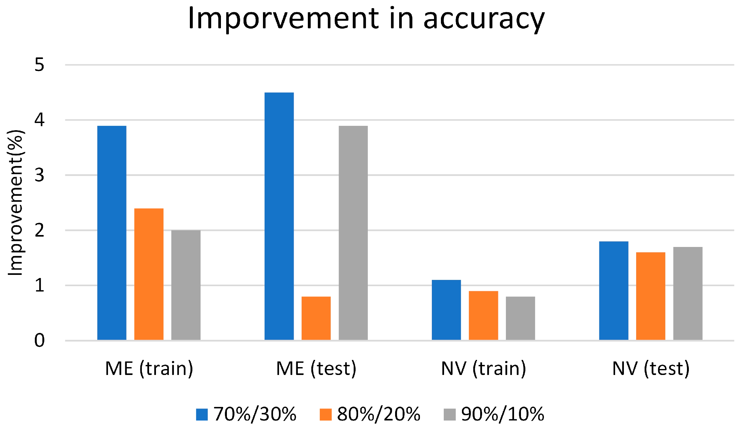
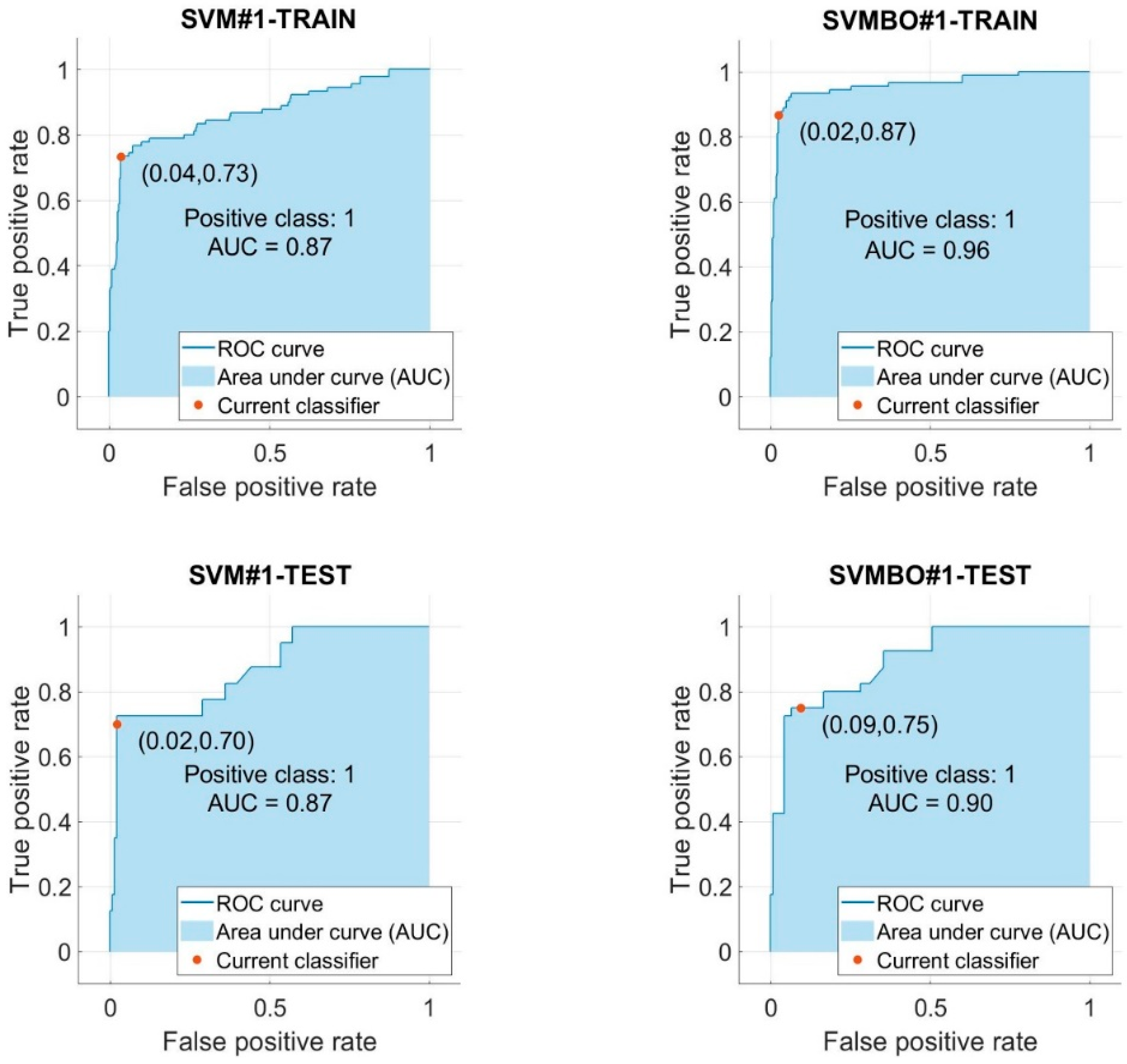
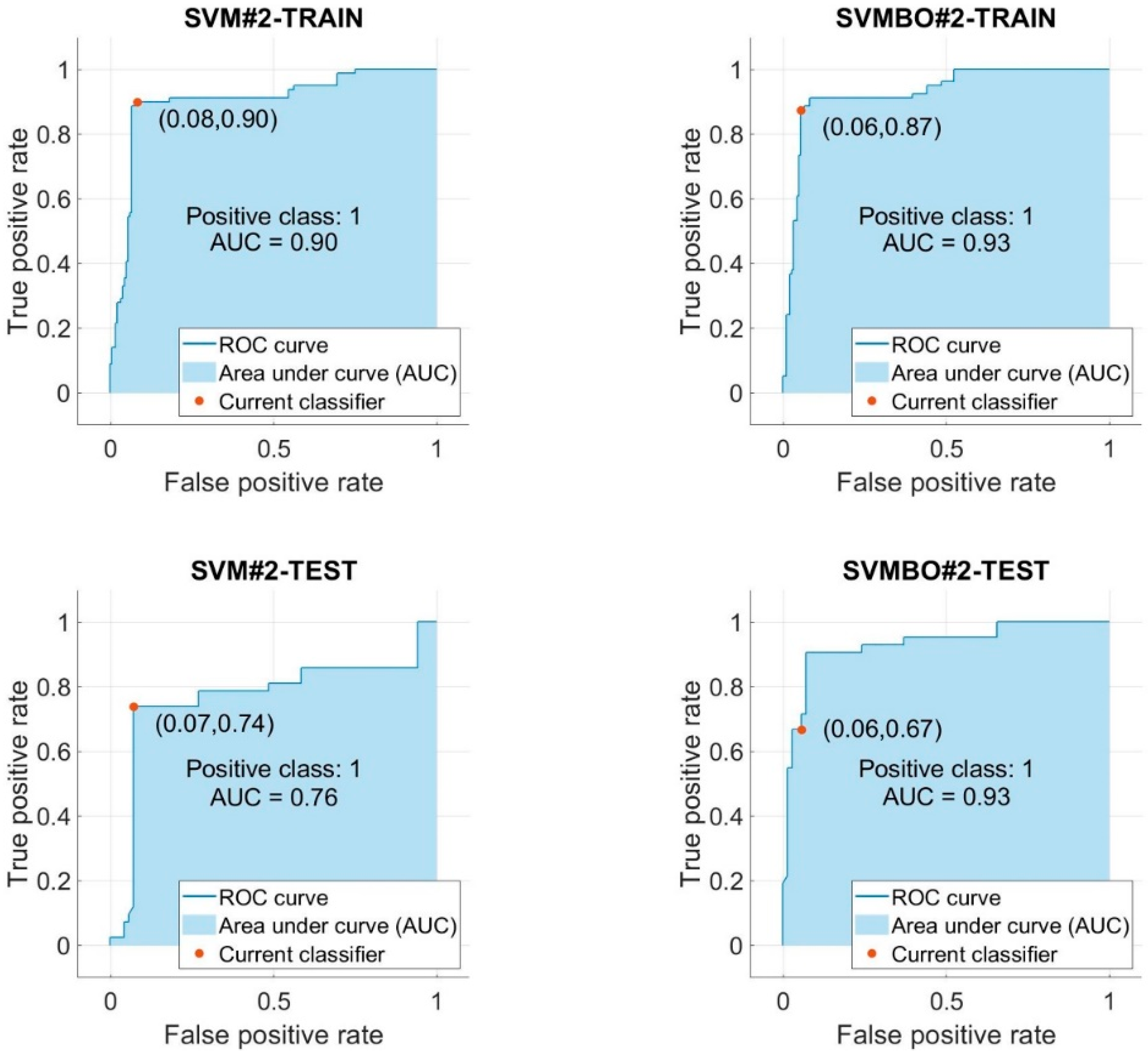
- The SVMBO approach outperformed the traditional SVM model in predicting the HVO.
- The BO technique concluded that the Gaussian kernel was the best kernel function for both datasets.
- The BO method enhanced the performance of the SVM#1 model by 4.27% and 5.16%, respectively, throughout the training and testing phases.
- For the SVM#2 model, the performance of this model was improved by 1.20% and 2.14% for the training and testing phases, correspondingly.
- The AUC of the SVM models used to predict the HVO was improved by using the BO technique.
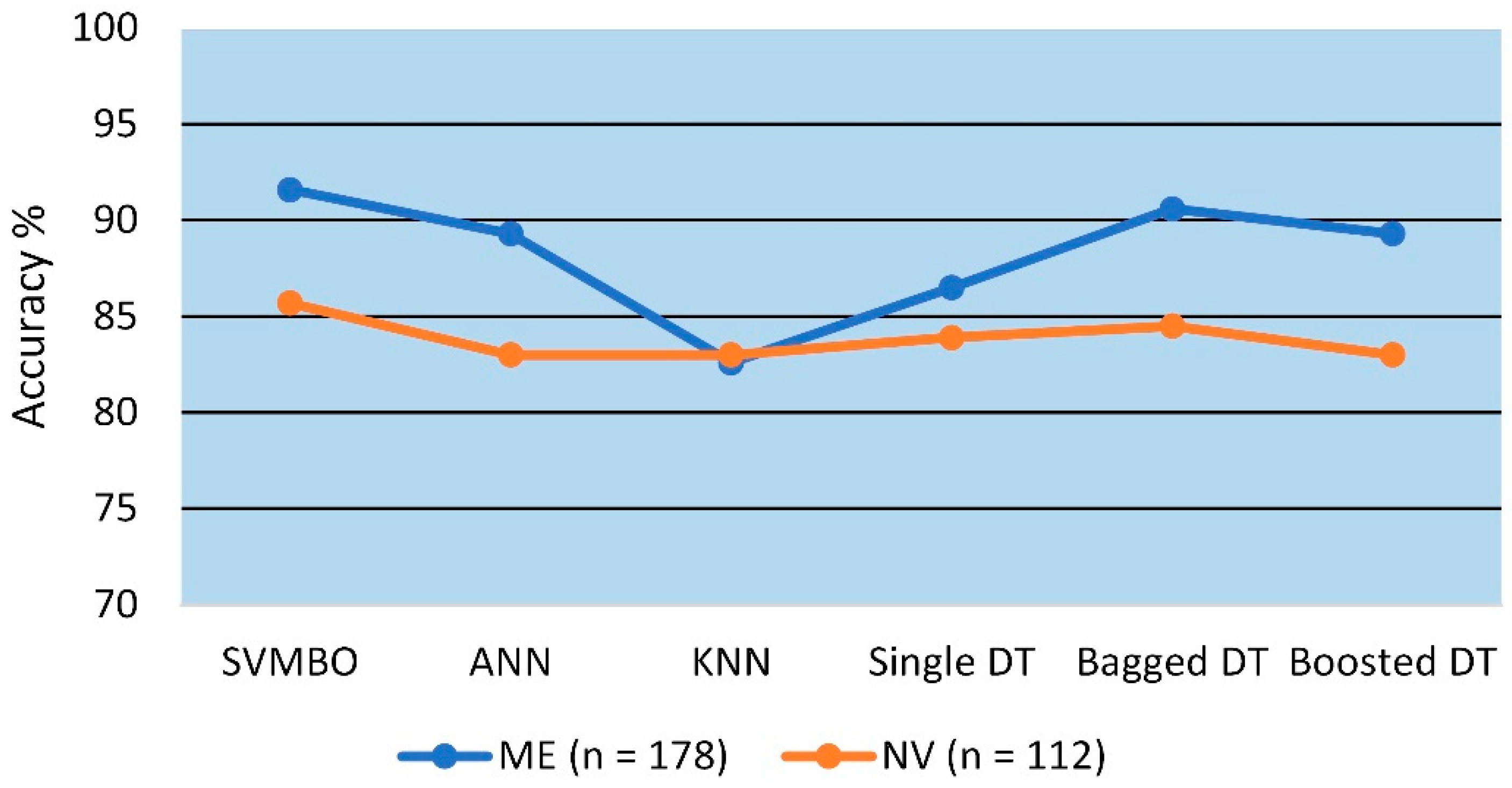
- In this study, the optimized SVM models did better than the other machine learning models that were applied.
Author Contributions
Funding
Institutional Review Board Statement
Informed Consent Statement
Acknowledgments
Conflicts of Interest
References
- Jain, T.; Rose, G.; Johnson, M. Changes in private car ownership associated with car sharing: Gauging differences by residential location and car share typology. Transportation 2022, 49, 503–527. [Google Scholar] [CrossRef] [PubMed]
- Zhou, F.; Zheng, Z.; Whitehead, J.; Perrons, R.K.; Washington, S.; Page, L. Examining the impact of car-sharing on private vehicle ownership. Transp. Res. A Policy Pract. 2020, 138, 322–341. [Google Scholar] [CrossRef]
- Bureau of Transportation Statistics. National Household Travel Survey Daily Travel Quick Facts. Available online: https://www.bts.gov/statistical-products/surveys/national-household-travel-survey-daily-travel-quick-facts (accessed on 1 April 2022).
- Handy, S.L.; Boarnet, M.G.; Ewing, R.; Killingsworth, R.E. How the built environment affects physical activity: Views from urban planning. Am. J. Prev. Med. 2002, 23, 64–73. [Google Scholar] [CrossRef]
- Zhao, P.; Zhang, Y. Travel behaviour and life course: Examining changes in car use after residential relocation in Beijing. J. Transp. Geogr. 2018, 73, 41–53. [Google Scholar] [CrossRef]
- Manjushree, N.; GH, S.G.; Swamy, S.C.; Giridharan, A. Household Vehicle Ownership Prediction Using Machine Learning Approach. In Proceedings of the 2022 International Conference for Advancement in Technology (ICONAT), Goa, India, 21–22 January 2022; pp. 1–8. [Google Scholar]
- Golroudbary, S.R.; Zahraee, S.M.; Awan, U.; Kraslawski, A. Sustainable Operations Management in Logistics Using Simulations and Modelling: A Framework for Decision Making in Delivery Management. Procedia Manuf. 2019, 30, 627–634. [Google Scholar] [CrossRef]
- Rashidi, S.; Ranjitkar, P.; Hadas, Y. Modeling bus dwell time with decision tree-based methods. Transp. Res. Rec. 2014, 2418, 74–83. [Google Scholar] [CrossRef]
- Stylianou, K.; Dimitriou, L.; Abdel-Aty, M. Big data and road safety: A comprehensive review. In Mobility Patterns, Big Data and Transport Analytics; Elsevier: Amsterdam, The Netherlands, 2019; pp. 297–343. [Google Scholar]
- Yan, X.; Richards, S.; Su, X. Using hierarchical tree-based regression model to predict train–vehicle crashes at passive highway-rail grade crossings. Accid. Anal. Prev. 2010, 42, 64–74. [Google Scholar] [CrossRef]
- Wahab, L.; Jiang, H. A comparative study on machine learning based algorithms for prediction of motorcycle crash severity. PLoS ONE 2019, 14, e0214966. [Google Scholar] [CrossRef]
- Wang, Y.; Zheng, Y.; Xue, Y. Travel Time Estimation of a Path Using Sparse Trajectories. In Proceedings of the 20th ACM SIGKDD International Conference on Knowledge Discovery and Data Mining, New York, NY, USA, 24–27 August 2014; pp. 25–34. [Google Scholar]
- Asif, M.T.; Mitrovic, N.; Dauwels, J.; Jaillet, P. Matrix and tensor based methods for missing data estimation in large traffic networks. IEEE Trans. Intell. Transp. Syst. 2016, 17, 1816–1825. [Google Scholar] [CrossRef]
- Kaewwichian, P. Multiclass Classification with Imbalanced Datasets for Car Ownership Demand Model–Cost-Sensitive Learning. Promet-Traffic Transp. 2021, 33, 361–371. [Google Scholar] [CrossRef]
- Nowicki, R.K.; Grzanek, K.; Hayashi, Y. Rough support vector machine for classification with interval and incomplete data. J. Artif. Intell. Soft Comput. Res. 2020, 10, 47–56. [Google Scholar] [CrossRef]
- Brand, L.; Baker, L.Z.; Wang, H. A Multi-Instance Support Vector Machine with Incomplete Data for Clinical Outcome Prediction of COVID-19. In Proceedings of the 12th ACM Conference on Bioinformatics, Computational Biology, and Health Informatics, Gainesville, FL, USA, 1–4 August 2021; pp. 1–6. [Google Scholar]
- Mohamed, M.; Cheffena, M. Received Signal Strength Based Gait Authentication. IEEE Sens. J. 2018, 18, 6727–6734. [Google Scholar] [CrossRef]
- Harrison, L.R.; Legleiter, C.J.; Overstreet, B.T.; Bell, T.W.; Hannon, J. Assessing the potential for spectrally based remote sensing of salmon spawning locations. River Res. Appl. 2020, 36, 1618–1632. [Google Scholar] [CrossRef]
- Qian, Y.; Aghaabbasi, M.; Ali, M.; Alqurashi, M.; Salah, B.; Zainol, R.; Moeinaddini, M.; Hussein, E.E. Classification of Imbalanced Travel Mode Choice to Work Data Using Adjustable SVM Model. Appl. Sci. 2021, 11, 11916. [Google Scholar] [CrossRef]
- Zhang, X.-H.; Hu, M.-Q.; Peng, X.-Y.; Gan, J.; Xiang, Q.-J. Prediction of Motor Vehicle Ownership in County Towns Based on Support Vector Machine. In Proceedings of the 2019 4th International Conference on Intelligent Transportation Engineering (ICITE), Singapore, 5–7 September 2019; pp. 311–315. [Google Scholar]
- Dou, J.; Yunus, A.P.; Bui, D.T.; Merghadi, A.; Sahana, M.; Zhu, Z.; Chen, C.-W.; Han, Z.; Pham, B.T. Improved landslide assessment using support vector machine with bagging, boosting, and stacking ensemble machine learning framework in a mountainous watershed, Japan. Landslides 2020, 17, 641–658. [Google Scholar] [CrossRef]
- Zhao, X.; Chen, W. Optimization of computational intelligence models for landslide susceptibility evaluation. Remote Sens. 2020, 12, 2180. [Google Scholar] [CrossRef]
- Li, J.; Walker, J.L.; Srinivasan, S.; Anderson, W.P. Modeling private car ownership in China: Investigation of urban form impact across megacities. Transp. Res. Rec. 2010, 2193, 76–84. [Google Scholar] [CrossRef]
- Song, S.; Diao, M.; Feng, C.-C. Effects of pricing and infrastructure on car ownership: A pseudo-panel-based dynamic model. Transp. Res. A Policy Pract. 2021, 152, 115–126. [Google Scholar] [CrossRef]
- Dargay, J.M.; Madre, J.-L.; Berri, A. Car ownership dynamics seen through the follow-up of cohorts: Comparison of France and the United Kingdom. Transp. Res. Rec. 2000, 1733, 31–38. [Google Scholar] [CrossRef]
- Yang, Z.; Jia, P.; Liu, W.; Yin, H. Car ownership and urban development in Chinese cities: A panel data analysis. J. Transp. Geogr. 2017, 58, 127–134. [Google Scholar] [CrossRef]
- Ruas, E.B. The Influence of Shared Mobility and Transportation Policies on Vehicle Ownership: Analysis of Multifamily Residents in Portland, Oregon. Ph.D. Dissertation, Portland State University, Portland, OR, USA, 2019. [Google Scholar]
- Cirillo, C.; Liu, Y. Vehicle ownership modeling framework for the state of Maryland: Analysis and trends from 2001 and 2009 NHTS data. J. Urban Plan. Dev. 2013, 139, 1–11. [Google Scholar] [CrossRef]
- Chu, M.Y.; Law, T.H.; Hamid, H.; Law, S.H.; Lee, J.C. Examining the effects of urbanization and purchasing power on the relationship between motorcycle ownership and economic development: A panel data. Int. J. Transp. Sci. Technol. 2020, 11, 72–82. [Google Scholar] [CrossRef]
- Dargay, J.; Hanly, M. Volatility of car ownership, commuting mode and time in the UK. Transp. Res. A Policy Pract. 2007, 41, 934–948. [Google Scholar] [CrossRef]
- Bhat, C.R.; Paleti, R.; Pendyala, R.M.; Lorenzini, K.; Konduri, K.C. Accommodating Immigration Status and Self-Selection Effects in a Joint Model of Household Auto Ownership and Residential Location Choice. Transp. Res. Rec. 2013, 2382, 142–150. [Google Scholar] [CrossRef]
- Li, S.; Zhao, P. Exploring car ownership and car use in neighborhoods near metro stations in Beijing: Does the neighborhood built environment matter? Transp. Res. D Transp. Environ. 2017, 56, 1–17. [Google Scholar] [CrossRef]
- Huang, X.; Cao, X.J.; Yin, J.; Cao, X. Effects of metro transit on the ownership of mobility instruments in Xi’an, China. Transp. Res. D Transp. Environ. 2017, 52, 495–505. [Google Scholar] [CrossRef]
- Matas, A.; Raymond, J.-L.; Roig, J.-L. Car ownership and access to jobs in Spain. Transp. Res. A Policy Pract. 2009, 43, 607–617. [Google Scholar] [CrossRef]
- Tyrinopoulos, Y.; Antoniou, C. Factors affecting modal choice in urban mobility. Eur. Transp. Res. Rev. 2013, 5, 27–39. [Google Scholar] [CrossRef]
- Sabouri, S.; Brewer, S.; Ewing, R. Exploring the relationship between ride-sourcing services and vehicle ownership, using both inferential and machine learning approaches. Landsc. Urban Plan. 2020, 198, 103797. [Google Scholar] [CrossRef]
- Jong, G.D.; Fox, J.; Daly, A.; Pieters, M.; Smit, R. Comparison of car ownership models. Transp. Rev. 2004, 24, 379–408. [Google Scholar] [CrossRef]
- Anowar, S.; Eluru, N.; Miranda-Moreno, L.F. Alternative modeling approaches used for examining automobile ownership: A comprehensive review. Transp. Rev. 2014, 34, 441–473. [Google Scholar] [CrossRef]
- Karlaftis, M.G.; Vlahogianni, E.I. Statistical methods versus neural networks in transportation research: Differences, similarities and some insights. Transp. Res. C Emerg. Technol. 2011, 19, 387–399. [Google Scholar] [CrossRef]
- Aghaabbasi, M.; Shekari, Z.A.; Shah, M.Z.; Olakunle, O.; Armaghani, D.J.; Moeinaddini, M. Predicting the use frequency of ride-sourcing by off-campus university students through random forest and Bayesian network techniques. Transp. Res. A Policy Pract. 2020, 136, 262–281. [Google Scholar] [CrossRef]
- Basu, R.; Ferreira, J. Understanding household vehicle ownership in Singapore through a comparison of econometric and machine learning models. Transp. Res. Procedia 2020, 48, 1674–1693. [Google Scholar] [CrossRef]
- Abdul Muhsin Zambang, M.; Jiang, H.; Wahab, L. Modeling vehicle ownership with machine learning techniques in the Greater Tamale Area, Ghana. PLoS ONE 2021, 16, e0246044. [Google Scholar] [CrossRef]
- Ha, T.V.; Asada, T.; Arimura, M. Determination of the influence factors on household vehicle ownership patterns in Phnom Penh using statistical and machine learning methods. J. Transp. Geogr. 2019, 78, 70–86. [Google Scholar] [CrossRef]
- Ma, T.; Aghaabbasi, M.; Ali, M.; Zainol, R.; Jan, A.; Mohamed, A.M.; Mohamed, A. Nonlinear Relationships between Vehicle Ownership and Household Travel Characteristics and Built Environment Attributes in the US Using the XGBT Algorithm. Sustainability 2022, 14, 3395. [Google Scholar] [CrossRef]
- Mohammadian, A.; Miller, E.J. Nested logit models and artificial neural networks for predicting household automobile choices: Comparison of performance. Transp. Res. Rec. 2002, 1807, 92–100. [Google Scholar] [CrossRef]
- Pineda-Jaramillo, J. Travel time, trip frequency and motorised-vehicle ownership: A case study of travel behaviour of people with reduced mobility in Medellín. J. Transp. Health 2021, 22, 101110. [Google Scholar] [CrossRef]
- Chaipanha, W.; Kaewwichian, P. Smote vs. Random Undersampling for Imbalanced Data-Car Ownership Demand Model. Communications 2022, 24, D105–D115. [Google Scholar] [CrossRef]
- Shao, Q.; Zhang, W.; Cao, X.J.; Yang, J. Nonlinear and interaction effects of land use and motorcycles/E-bikes on car ownership. Transp. Res. D Transp. Environ. 2022, 102, 103115. [Google Scholar] [CrossRef]
- Wang, X.; Pan, Z.; Wang, H.; Lu, Z.; Huang, J.; Yu, X. Forecast of Electric Vehicle Ownership Based on MIFS-AdaBoost Model. In Proceedings of the 2021 IEEE 4th International Conference on Automation, Electronics and Electrical Engineering (AUTEEE), Shenyang, China, 19–21 November 2021; pp. 4–8. [Google Scholar]
- Tanwanichkul, L.; Kaewwichian, P.; Pitaksringkarn, J. Car ownership demand modeling using machine learning: Decision trees and neural networks. GEOMATE J. 2019, 17, 219–230. [Google Scholar]
- Bas, J.; Cirillo, C.; Cherchi, E. Classification of potential electric vehicle purchasers: A machine learning approach. Technol. Forecast. Soc. Chang. 2021, 168, 120759. [Google Scholar] [CrossRef]
- Kash, G.; Mokhtarian, P.L. What Counts as Commute Travel? Identification and Resolution of Key Issues around Measuring Complex Commutes in the National Household Travel Survey. Transp. Res. Rec. 2021, 2676, 03611981211051346. [Google Scholar] [CrossRef]
- Sadeghvaziri, E.; Tawfik, A. Using the 2017 National Household Travel Survey Data to Explore the Elderly’s Travel Patterns. In Proceedings of the International Conference on Transportation and Development 2020, Seattle, WA, USA, 26–29 May 2020; pp. 86–94. [Google Scholar]
- Esekhaigbe, E.O.; Bills, T. Examining the Travel Behavior of Transport Disadvantaged Communities Using the 2017 National Household Travel Survey. In Proceedings of the Transportation Research Board 100th Annual Meeting, Washington, DC, USA, 5–29 January 2021. [Google Scholar]
- Kickhöfer, B.; Bahamonde-Birke, F.J.; Nordenholz, F. Dynamic modeling of vehicle purchases and vehicle type choices from national household travel survey data. Transp. Res. Procedia 2019, 41, 2–5. [Google Scholar] [CrossRef]
- Cortes, C.; Vapnik, V. Support-vector networks. Mach. Learn. 1995, 20, 273–297. [Google Scholar] [CrossRef]
- Chang, C.-C.; Lin, C.-J. LIBSVM: A library for support vector machines. ACM Trans. Intell. Syst. Technol. (TIST) 2011, 2, 27. [Google Scholar] [CrossRef]
- Smola, A.J.; Schölkopf, B. A tutorial on support vector regression. Stat. Comput. 2004, 14, 199–222. [Google Scholar] [CrossRef]
- Snoek, J.; Larochelle, H.; Adams, R.P. Practical bayesian optimization of machine learning algorithms. Adv. Neural Inf. Process. Syst. 2012, 25, 1–9. [Google Scholar]
- Greenhill, S.; Rana, S.; Gupta, S.; Vellanki, P.; Venkatesh, S. Bayesian optimization for adaptive experimental design: A review. IEEE Access 2020, 8, 13937–13948. [Google Scholar] [CrossRef]
- Kobliha, M.; Schwarz, J.; Očenášek, J. Bayesian optimization algorithms for dynamic problems. In Proceedings of the Workshops on Applications of Evolutionary Computation, Budapest, Hungary, 10–12 April 2006; pp. 800–804. [Google Scholar]
- Yu, Q.; Monjezi, M.; Mohammed, A.S.; Dehghani, H.; Armaghani, D.J.; Ulrikh, D.V. Optimized Support Vector Machines Combined with Evolutionary Random Forest for Prediction of Back-Break Caused by Blasting Operation. Sustainability 2021, 13, 12797. [Google Scholar] [CrossRef]
- Ke, B.; Khandelwal, M.; Asteris, P.G.; Skentou, A.D.; Mamou, A.; Armaghani, D.J. Rock-Burst Occurrence Prediction Based on Optimized Naïve Bayes Models. IEEE Access 2021, 9, 91347–91360. [Google Scholar] [CrossRef]
- Merghadi, A.; Yunus, A.P.; Dou, J.; Whiteley, J.; ThaiPham, B.; Bui, D.T.; Avtar, R.; Abderrahmane, B. Machine learning methods for landslide susceptibility studies: A comparative overview of algorithm performance. Earth-Sci. Rev. 2020, 207, 103225. [Google Scholar] [CrossRef]
- Rashedi, E.; Nezamabadi-Pour, H.; Saryazdi, S. GSA: A gravitational search algorithm. Inf. Sci. 2009, 179, 2232–2248. [Google Scholar] [CrossRef]
- Abdel-Basset, M.; Shawky, L.A. Flower pollination algorithm: A comprehensive review. Artif. Intell. Rev. 2019, 52, 2533–2557. [Google Scholar] [CrossRef]
- Kleinberg, J.; Ludwig, J.; Mullainathan, S.; Obermeyer, Z. Prediction policy problems. Am. Econ. Rev. 2015, 105, 491–495. [Google Scholar] [CrossRef] [PubMed] [Green Version]


| Variable | Description | Type |
|---|---|---|
| Independent variable | ||
| HHVEHCNT | The number of household vehicles | Binary (1, >1) |
| Dependent variables | ||
| HHFAMINC | Income of household ($) | Categorial |
| SIZE | Size of household | Continuous |
| HOMEOWN | Home ownership | Binary |
| NUMADLT | How many adults live in the household? | Continuous |
| WRKCOUNT | How many workers does the household have? | Continuous |
| YOUNGCHILD | How many children live in the household? | Continuous |
| DRVRCNT | How many drivers does a household have? | Continuous |
| TRPHHACC | How many household members are on the trip? | Continuous |
| TRPHHVEH | Is the household vehicle used for the trip? | Binary |
| BIKE_DFR | How inadequate is bicycle infrastructure? | Categorial |
| HBPPOPDN | Density of population | Categorial |
| URBANSIZE | What is the size of the urban area around the household? | Categorial |
| URBRUR | Does the household live in an urban or rural area? | Binary |
| WALK_DEF | How inadequate is walking infrastructure? | Categorial |
| Dataset | Model | Train | Test | |||||
|---|---|---|---|---|---|---|---|---|
| Actual | Prediction | Accuracy (%) | Prediction | Accuracy (%) | ||||
| 1 | 2 | 1 | 2 | |||||
| ME dataset | SVM#1 | 1 | 66 | 24 | 91.3 | 30 | 10 | 87.1 |
| 2 | 12 | 312 | 13 | 125 | ||||
| SVMBO#1 | 1 | 78 | 12 | 95.2 | 28 | 12 | 91.6 | |
| 2 | 8 | 316 | 3 | 135 | ||||
| NV dataset | SVM#2 | 1 | 71 | 8 | 91.2 | 28 | 14 | 83.9 |
| 2 | 15 | 166 | 4 | 66 | ||||
| SVMBO#2 | 1 | 69 | 10 | 92.3 | 31 | 11 | 85.7 | |
| 2 | 10 | 171 | 5 | 65 | ||||
| SVM#1 | SVMBO#1 | SVM#2 | SVMBO#2 | |
|---|---|---|---|---|
| Population size * | 414 | 414 | 260 | 260 |
| Kernel function | - | Gaussian | - | Gaussian |
| Gamma | - | 5.3103 | - | 4.1209 |
| C | - | 53.4787 | - | 9.4636 |
| Training time (sec) | 1.2986 | 324.5 | 3.8578 | 424.6 |
Publisher’s Note: MDPI stays neutral with regard to jurisdictional claims in published maps and institutional affiliations. |
© 2022 by the authors. Licensee MDPI, Basel, Switzerland. This article is an open access article distributed under the terms and conditions of the Creative Commons Attribution (CC BY) license (https://creativecommons.org/licenses/by/4.0/).
Share and Cite
Xu, Z.; Aghaabbasi, M.; Ali, M.; Macioszek, E. Targeting Sustainable Transportation Development: The Support Vector Machine and the Bayesian Optimization Algorithm for Classifying Household Vehicle Ownership. Sustainability 2022, 14, 11094. https://doi.org/10.3390/su141711094
Xu Z, Aghaabbasi M, Ali M, Macioszek E. Targeting Sustainable Transportation Development: The Support Vector Machine and the Bayesian Optimization Algorithm for Classifying Household Vehicle Ownership. Sustainability. 2022; 14(17):11094. https://doi.org/10.3390/su141711094
Chicago/Turabian StyleXu, Zhiqiang, Mahdi Aghaabbasi, Mujahid Ali, and Elżbieta Macioszek. 2022. "Targeting Sustainable Transportation Development: The Support Vector Machine and the Bayesian Optimization Algorithm for Classifying Household Vehicle Ownership" Sustainability 14, no. 17: 11094. https://doi.org/10.3390/su141711094