Forecasting Photovoltaic Power Generation with a Stacking Ensemble Model

Abstract

Nowadays, photovoltaics (PV) has gained popularity among other renewable energy sources because of its excellent features. However, the instability of the system’s output has become a critical problem due to the high PV penetration into the existing distribution system. Hence, it is essential to have an accurate PV power output forecast to integrate more PV systems into the grid and to facilitate energy management further. In this regard, this paper proposes a stacked ensemble algorithm (Stack-ETR) to forecast PV output power one day ahead, utilizing three machine learning (ML) algorithms, namely, random forest regressor (RFR), extreme gradient boosting (XGBoost), and adaptive boosting (AdaBoost), as base models. In addition, an extra trees regressor (ETR) was used as a meta learner to integrate the predictions from the base models to improve the accuracy of the PV power output forecast. The proposed model was validated on three practical PV systems utilizing four years of meteorological data to provide a comprehensive evaluation. The performance of the proposed model was compared with other ensemble models, where RMSE and MAE are considered the performance metrics. The proposed Stack-ETR model surpassed the other models and reduced the RMSE by 24.49%, 40.2%, and 27.95% and MAE by 28.88%, 47.2%, and 40.88% compared to the base model ETR for thin-film (TF), monocrystalline (MC), and polycrystalline (PC) PV systems, respectively.

1. Introduction

Currently, power plants employ traditional energy sources, including fossil fuel, gas, and coal, to generate electricity. Unfortunately, these sources significantly harm the environment by producing carbon dioxide (CO₂) and other toxic gases, contributing to global warming [1]. The problems of fossil energy pollution and energy scarcity are severely increasing as the social economy develops rapidly [2]. Due to their abundant and climate-friendly attributes, renewable energy resources are being introduced in the hope that they will mitigate these issues. Sustainable use and the growth of renewable and clean energy are primarily focused on wind and photovoltaics (PV), which are cost-effective, realistic, and feasible solutions to this challenge [3]. PV generation has already surpassed wind power generation as a new growth point in the renewable energy sector [4]. Because of the contrast between day and night illumination, photovoltaic generation is advantageous. However, regardless of PV’s advantages and the solutions it offers, PV generation is characterized by a high degree of uncertainty and an intermittent nature [5] due to the influence of climatic factors, such as cloudiness, temperature, and aerosols. In addition, the high PV penetration in the distribution system impacts the voltage at the buses negatively. A recent significant development in installing PV systems has resulted in reverse power flow along feeders, resulting in an overvoltage issue. During noon hours, when there is a large PV power injection but a low load demand, the overvoltage problem worsens significantly. It limits the power injection from not only PV systems but also any future integration of PV into the distribution system. These factors lead PV power generation that is grid-connected to affect the grid [6]. Consequently, if the PV output power could be accurately forecasted in real-time with insignificant delay, it would be essential for power grid dispatching or regulation and the steady operation of PV power stations [7] to maintain optimal planning and operation for the distribution networks [8,9,10]. Further, problems related to voltage regulation due to high PV penetration can be solved by taking into account the predictive power compensation [11] or by islanding the microgrids under limited communication to enhance the operation of the distribution system [12].

PV forecasting can be classified into four main horizons based on the period: ultra-short-, short-, medium-, and long-term forecasting [13]. In the case of ultra-short, forecasting is performed at the minute scale and can be defined as nowcasting, whereas short-term forecasting ranges from 48–72 h ahead. Finally, the medium- and long-term can vary between a few days to a week and a few months to a year or more, respectively [14]. When developing a power policy, the authority and decisionmakers focus primarily on long-term forecasting to account for future PV energy generation. On the other hand, utility companies mostly conduct short-term forecasting to establish a plan for electricity production, manage energy reserves, and assess purchase and sales agreements. In this study, the authors focused on a short-term, one-day-ahead PV power output forecasting model.

Forecasting techniques can be categorized into statistical and machine learning (ML) models. The statistical models mostly consist of auto-regression (AR), auto-regressive moving average (ARMA), autoregressive moving average with exogenous variable (ARMAX), and linear regression (LR). For instance, an ARMA model was proposed in [15] to forecast PV power output. Further, an ARMAX model was used in [16] to forecast the power generation of a PV system and verified by utilizing a grid-connected 2.1 kW PV system; the results showed that the ARMAX surpassed the ARMA by attaining better accuracy. A vector autoregression approach was presented in [17]; the main aim of the study was to forecast solar power six hours ahead utilizing distributed information. A short-term PV power forecasting system (up to 72 h ahead) utilizing a bottom-up framework and meteorological data was proposed in [18] to predict PV energy generation in Luxembourg. It is evident that statistical methods can be used to forecast PV power output, but these types of models are mainly based on linear relationships. In addition, they have restricted capabilities in showing nonlinear correlations.

ML was introduced and has gained more popularity for such applications to overcome these previous issues. ML differs from conventional statistical techniques in that it does not impose stringent criteria on data distribution, can handle high-dimensional data, and is straightforward in dimension reduction capability. Many researchers have developed robust solar PV forecast models based on the previous literature to focus on these concerns [19,20,21]. For example, the implementation of ensemble ML models, such as random forest (RF) [22], gradient boosting regression trees (GBRT) [23], and extreme gradient boosting (XGBoost) [24], has shown promising results in comparison to traditional models. Further, ensemble approaches are more stable and can decrease the uncertainty related to the input data [25]. For instance, Usman and Zhanle [26] developed a framework for assessing several ML techniques comprising RF, XGBoost, and artificial neural network (ANN), with feature selection algorithms to forecast short-term PV power generation. According to them, XGBoost is superior in contrast to other machine learning algorithms.

Nevertheless, since PV generation is characterized by periods of high variability on partly cloudy days and low variability on sunny days; the meteorological data for a given location are not always precise enough to forecast these periods with precision. To overcome this problem, Andrade et al. [24] proposed a forecasting framework by combining XGboost with feature engineering techniques. However, most studies have employed a single ML model, and the generalizability and reliability of these studies are still inadequate. Hybrid methods in ML are also generally used to deal with the single ML model’s drawbacks. For example, to forecast PV power one hour in advance, hybrid RF-PCA-K-means-HGWO [27] was used; the proposed model achieved MAE values 0.18, 0.14, and 0.19 percent lower than the optimal findings of the previous models. The short-term forecasting of PV power output was discussed in [28], and the RF-CEEMD-DIFPSOBPNN model was developed to enhance the forecasting performance under different weather conditions, including the sunny, cloudy, and rainy seasons. The proposed model also coped with the drawbacks of single models.

Recently, scholars have developed diverse ensemble learning models, including bagging, boosting, and stacking. Compared to the bagging and boosting methods, the stacking approach is distinguished by two primary aspects. First, the stacking model typically accounts for heterogeneous base learners (various learning methods are coupled), whereas bagging and boosting mostly account for homogeneous base learners. The stacking model integrates base models with the meta-model, whereas bagging and boosting incorporate base learners using deterministic algorithms. For instance, various stacking models were proposed in [29], utilizing different datasets for forecasting the PV output power production; the results disclosed that the Stacking-GBDT model performed better compared with other stacking models, achieving RMSE and MAE values with 47.7826 and 106.07, respectively. Further, staking XGBoost was proposed in [25] to predict PV output generation, whereas a stacking ensemble model with a recurrent neural network (RNN) as a meta-learner was discussed in [30] for one-to-three-day ahead PV power forecasting. The authors of [31] proposed five models of LSTM, such as LSTM with time step, LSTM using the window method, and stacked LSTM. The results showed that LSTM with time step achieved the lowest RSME. A hybrid model based on XGBoost and ANN that integrated its output using ridge regression was presented in [32]. Additionally, the authors concluded that hybrid models are more accurate and stable than single models. Recently, the authors of [33] suggested using RNN-LSTM to forecast the PV power output for three different PV systems; compared with other models, the proposed model achieved the lowest RMSE values, where the values attained were 39.2, 19.78, and 26.85 for TF, MC, and PV, respectively.

Table 1. Highlighting the considered parameters in the recent works from the literature.

Ref	Model	Input Variables	Horizon	PV Module			Dataset Duration	Target
				MC	PC	TF
[29]	Stacking-GBDT	Light intensity, wind speed and direction, weather temperature, PV module temperature, transfer efficiency	Ultra-short-term (5 min ahead)	Not mentioned			4 years	PV power output
[32]	XGBoost-DNN	Temperature, pressure, wind speed and direction, relative humidity, month number, clear sky index, time	Short-term (1 h ahead)	Not included			10 years	Solar irradiance
[33]	RNN-LSTM	Time, solar irradiance, wind speed, ambient temperature, PV module temperature, actual output power	Short-term (1 h ahead)	✓	✓	✓	4 years	PV power output
[34]	ELM	Solar irradiance, wind speed, ambient temperature, PV module temperature, actual output power	Short-term (1 day ahead and 1 h ahead)	✓	✓	✓	1 year	PV power output
[31]	LSTM-RNN	Actual output power	Short-term (1 h ahead)	Not mentioned			1 year	PV power output
[35]	LSTM	Actual output power and sky images	Ultra-short-term (1, 2, 5, 10 min ahead)	Not mentioned			Not mentioned	PV power output
[36]	DPNN	Temperature, wind speed and direction, relative humidity, sky condition, time, solar irradiance, sea level pressure	Short-term (1-9 h ahead)	✓	✕	✕	2 weeks	PV power output
[37]	DSE-XGB	Hour, day, month, previous day, same-time historical PV generation, previous 15 min, previous hour, solar irradiance, relative humidity, temperature	Ultra-short and short-term (15 min and 1 h ahead)	✓	✕	✕	3 years	PV power output
Proposed Research	Stacking-ETR	Time, solar irradiance, wind speed, ambient temperature, PV module temperature, actual output power	Short-term (1 day ahead)	✓	✓	✓	4 years	PV power output

summarizes the main differences between previous works and the proposed work in different aspects, including input variables, forecasting horizon, PV module type, dataset duration, and primary target.

Most prior research on the ML ensemble model approached solar PV production as a regression task by employing statistical models and random forest at the base level [32,38,39]. However, the dynamic nature of solar PV timeseries data, with its weather dependence and autoregressiveness, makes them difficult to predict using solely computational intelligence techniques such as the single ensemble model. Moreover, they are ineffective at recognizing nonlinear timeseries behavior and have poor prediction abilities. Therefore, to overcome these limitations, this research employed a one-level stack ensemble model, including the RFR, ETR, XGBoost, and Adaboost models. This study utilized XGBoost’s ability to capture data characteristics in PV power forecasting, AdaBoost’s capacity for prediction tasks with low bias errors while not being easily overfitted during training, and RFR’s superior fitting ability and high tolerance for poor information. In addition, the ensemble ML technique ETR was used to aggregate each base model’s prediction. Utilizing ETR as a meta-learner included quantifying individual model errors and data noise uncertainty, resulting in better prediction accuracy.

The contribution of this study to the literature can be summarized as follows:

• An ensemble stacking model (Stack-ETR) was developed that can be utilized as a baseline model for one-day-ahead PV power output forecasts, utilizing metrological data without heavy hyperparameter tuning.
• A performance evaluation of the proposed Stack-ETR was conducted on three different actual Malaysian PV systems over four years (2018 to 2021).
• In addition, the proposed model was compared with existing models and works to highlight the superiority of the proposed model.

This paper’s remaining sections are structured as follows: Section 2 offers the conceptual underpinning for constructing the stacked ensemble model. Section 3 presents the modeling outcomes, and Section 4 discusses broad directions and issues for future research.

2. Methodology

This part of the paper explains the proposed methodology and comprehensively explains the development of the proposed Stacking-ETR model. After developing the Stacking-ETR model, the validation of the proposed model was conducted on three practical Malaysian PV systems. In addition, the performance was evaluated using performance metrics. The data collection and processing were performed at the Power Electronics and Renewable Energy Research Laboratory (PEARL) at the University of Malaya, which included an overview of the grid-linked PV system installed on the engineering tower roof. The sequence of stages necessary for creating and assessing the proposed model is depicted in Figure 1.

2.1. The Machine Learning Models

The methodologies used in this investigation are described in this section. This method evaluates and categorizes supervised learning techniques for several independent variables into three groups: bagging and boosting ensemble approaches, as well as the proposed Stack-ETR model.

2.1.1. Bagging Ensemble Model

An ensemble of regressions aims to develop a more efficient model by combining the results of many regression models. Bagging ensemble also reduces the model’s variance and trains weak models in parallel. Random forest regressor (RFR) and extra trees regressor (ETR) are the most common bagging methods.

Random Forest Regressor (RFR)

The RFR is an ensemble-based machine learning technique based on the bagging approach, which combines many trees. In RFR, a voting mechanism is used to improve the performance of several base learners, decision trees (DT) in this study. The distinguishing characteristics of random forest are bootstrap sampling, random feature selection, out-of-bag (OOB) error estimation, and full-depth DT construction [39,40]. The RFR is built from a series of decision trees. For instance, classification and regression trees (CARTs) are one example of decision tree methods. A CART undergoes some enhancement when paired with the RFR. The RFR does not require cross-validation because it can perform out-of-bag error estimation natively throughout the forest construction process. It is asserted that OOB error estimation is impartial across numerous tests.

The training process for an RFR may be summed up as follows. In the first step, the RFR draws a bootstrap sample from the initial dataset. For each bootstrap sample obtained in the first step, it will develop an unpruned regression tree with the following modifications in the second step: At each node, it will take a random sample (n) of the input variables and determine the optimal split among them. After that, it will repeat steps 1 and 2 until the total number of identical trees has developed; then, it will forecast new data by averaging the predictions of the total trees’ numbers.

Extra Trees Regressor (ETR)

ETR, or extremely randomized trees, is a tree-based ensemble ML technique based on the bagging approach [41]. This approach was designed as an extension of the random forest algorithm and is relatively new. The ETR approach builds an ensemble of unpruned regression trees via a traditional top-down procedure. Like RFR, ETR uses a random selection of characteristics to train each base estimator. However, rather than picking the best split in each node, ETR chooses, at random, the best feature and matching value for dividing the node [38]. In addition, RFR uses bootstrap replication to train the prediction model, whereas ETR employs the entire training set to train every regression tree in the forest. These significant modifications reduce the likelihood that ET will overfit data, as a higher performance was documented in [41].

2.1.2. Boosting Ensemble Model

Boosting ensemble methods attempt to reduce the model’s bias by successively training several models to enhance each previously created model. The most common boosting methods are AdaBoost and XGBoost.

Extreme Gradient Boosting (XGBoost)

XGBoost is a supervised ensemble ML method based on boosted trees [42]. XGBoost is an enhanced and scalable implementation of the gradient boosting (GB) method that iteratively combines weak base models into a more robust model. XGBoost fits the input data to the first base model. Then, a second model is fitted to its residual to enhance the learning capacity of the first learner. This procedure of residue buildup is continued until the specified requirements are reached. The result is computed by aggregating the results of all the base models. It also prevents overfitting by integrating a regularization term into the goal function. GB’s learning process is quicker than XGBoost’s due to system optimization, parallel computing, and distributed computing [37]. GB utilizes a stopping criterion for tree splitting dependent on a negative loss criterion, whereas XGBoost applies a depth-first strategy. Using the maximum depth option, XGBoost prunes the tree reversely. In the XGBoost technique, sequential tree construction is accomplished through parallel implementation. XGBoost’s outer and inner loops are interchangeable. The inner loop computes a tree’s characteristics, while the outer loop enumerates its leaf nodes. This switching method improves the efficiency of the algorithm.

Adaptive Boosting (AdaBoost)

The AdaBoost ensemble ML algorithm is based on the boosting approach, and many algorithms were developed from its focus on classification and regression issues [43,44]. However, in contrast to other boosting algorithms, the AdaBoost method is an iterative algorithm that modifies the learning pattern based on the error produced by base learners. The core concept of the AdaBoost algorithm is to create a robust learner by merging weak base learners generated in each iteration; hence, it is crucial to weigh and combine base learners appropriately. Several models can be used as base learners in AdaBoost. The most common base learners used in AdaBoost are decision tree regression (DTR) and linear regression (LR). In this work, the authors utilized LR as a base learner for AdaBoost.

2.1.3. Stack Generalization

Stacked generalization, often known as stacking, is an additional ensemble learning approach developed by Wolpert [45] that has been utilized extensively in several domains since its creation. In stacking, the results of various models (random forest, AdaBoost, etc.) are stacked to train a new meta-learner for the final prediction. Stacking’s fundamental premise is built on two tiers of algorithms. The first level comprises several algorithms known as base learners, while the second is made of a meta-learner known as a stacking algorithm. First-level learners are frequently different base models; however, stack ensembles may also be constructed from the same base learner model [46]. First-level learners are trained to predict the result using the original dataset. Then, each base learner’s prediction is compiled to generate a new dataset. The new dataset comprises forecasts made by weak learners. Then, this dataset is utilized by the second-level meta-learner to produce the final prediction. The purpose of the meta-learner model is to correct the errors produced by the base models by adjusting the final output prediction. Multiple stacking layers are possible, with each level’s prediction serving as an input for the next. Stacking is the most advanced ensemble learning technique. It can effectively reduce both bias and variance by avoiding overfitting.

This work highlights the capacity of stacked machine learning models by presenting an adaptable implementation that considers ensemble architecture. The primary goal of stacking is to determine the optimal mix of models for the PV output power forecast. Therefore, four stack models are formed; the stack models are shown in Table 2. Ten-fold cross-validation of the base models was used to prepare the training dataset for the meta-model, while the out-of-fold predictions served as the basis for the training dataset. The entire process of the proposed Stack-ETR model is shown in Figure 2. The steps of the proposed Stack-ETR are elaborated as follows:

Step 1: The first step is data collection, including solar irradiance, ambient and PV module temperature, wind speed, time, and the actual power produced by the three types of PV.

Step 2: The next stage is data preprocessing and scaling. The collected data is daily averaged and scaled, as detailed in Section 2.2; the data is divided into training and testing sets, with a ratio of 80:20.

Step 3: The first level of the Stack-ETR consists of the base models (RFR, XGBoost, and AdaBoost). The base models predict the PV power output utilizing 10-fold cross-validation.

Step 4: The second level of the Stack-ETR consists of a meta-regressor (ETR), which takes all the predictions of base models as an input (M × P_i) to produce the final forecast.

Step 5: The proposed Stack-ETR model is evaluated using the performance metrics described in Section 2.2.

Table 2. Stack ensemble models.

Model Name	Base Learners	Meta-Learner
Stack-RFR	ETR, XGBoost, AdaBoost	RFR
Stack-ETR	RFR, XGBoost, AdaBoost	ETR
Stack-XGBoost	RFR, ETR, AdaBoost	XGBoost
Stack-AdaBoost	RFR, ETR, XGBoost	AdaBoost

Table 2. Stack ensemble models.

Model Name	Base Learners	Meta-Learner
Stack-RFR	ETR, XGBoost, AdaBoost	RFR
Stack-ETR	RFR, XGBoost, AdaBoost	ETR
Stack-XGBoost	RFR, ETR, AdaBoost	XGBoost
Stack-AdaBoost	RFR, ETR, XGBoost	AdaBoost

Figure 2. The entire process of the proposed Stack-ETR model.

Figure 2. The entire process of the proposed Stack-ETR model.

2.2. Performance Metrics Utilized to Assess the Model’s Effectiveness

Equations (1)–(4) assess the forecast accuracy for all models based on the evaluation metrics. The root mean square error (RMSE), as stated in Equation (1), is the first measurement metric. Mean square error (MSE) is described in Equation (2), while the coefficient of determination (R²) and mean absolute error (MAE) are stated in Equations (3) and (4), respectively. Finally, the values $P$ and $\widehat{P}$ represent the actual values and forecasted values, respectively. The value $P_{avg}$, on the other hand, represents the average of the actual values.

$$\mathrm{RMSE}=\sqrt{\frac{1}{H}{\displaystyle \sum }_{i=1}^H{\left(\widehat{P}-P\right)}^2}\hspace{1em}\hspace{1em}\hspace{1em}\hspace{1em}\left(\mathrm{Wh}/{\mathrm{m}}^2\right)$$

(1)

$$\mathrm{MSE}=\frac{1}{H}{\displaystyle \sum }_{i=1}^H{\left(\widehat{P}-P\right)}^2\hspace{1em}\hspace{1em}\hspace{1em}\hspace{1em}\hspace{1em}\hspace{1em}\hspace{1em}\left(\mathrm{Wh}/{\mathrm{m}}^2\right)$$

(2)

$$R^2=1-\frac{{{\displaystyle \sum }}_{i=1}^H{\left(\widehat{P}-P_{avg}\right)}^2}{{{\displaystyle \sum }}_{i=1}^H{\left(P-P_{avg}\right)}^2}$$

(3)

$$\mathrm{MAE}=\frac{1}{H}{\displaystyle \sum }_{i=1}^H|(\widehat{P}-P)|\hspace{1em}\hspace{1em}\hspace{1em}\hspace{1em}\hspace{1em}\hspace{1em}\left(\mathrm{Wh}/{\mathrm{m}}^2\right)$$

(4)

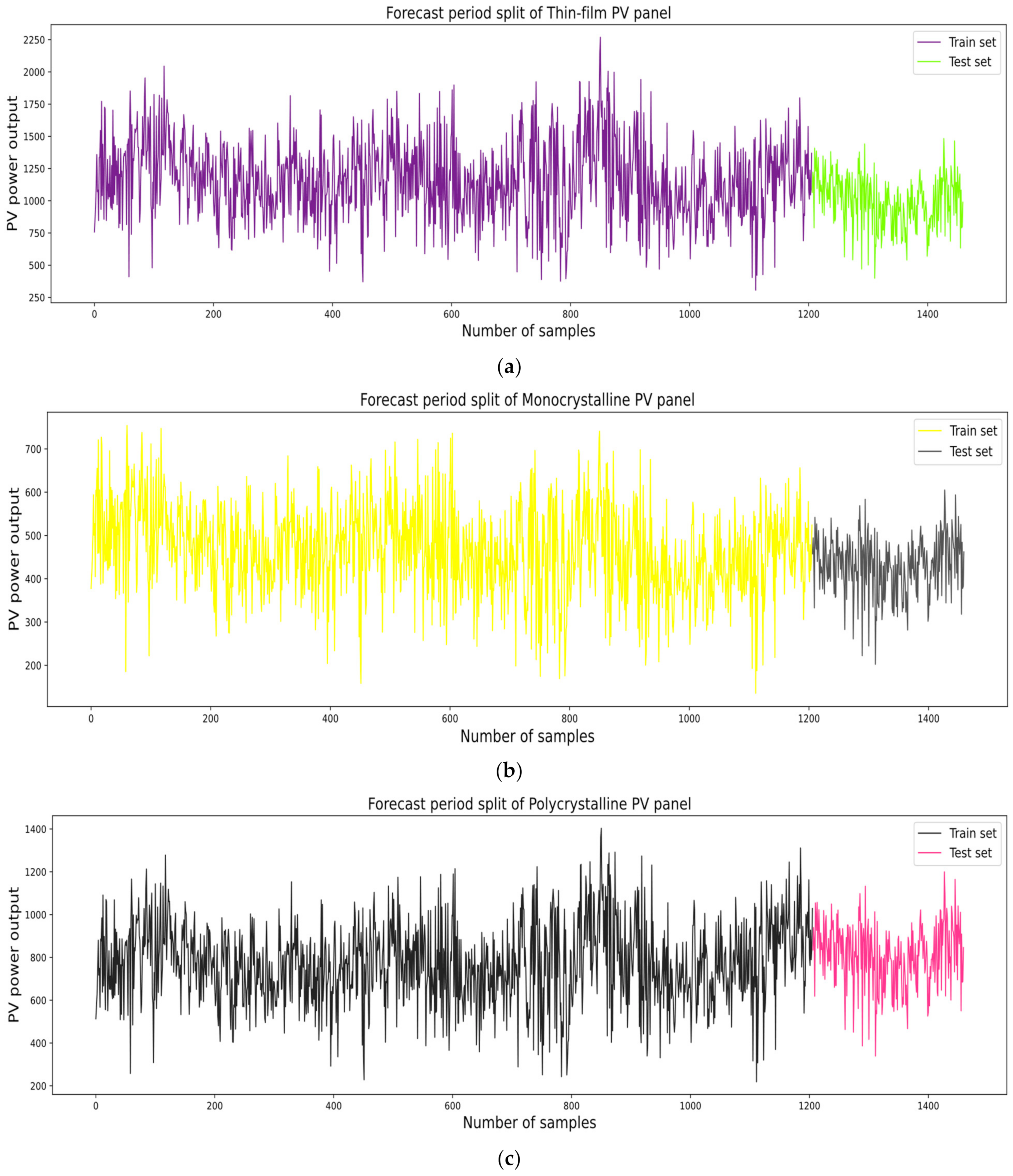
2.3. Data Preparation and Partitioning

Data preparation and partitioning confirmed the positive impacts on model convergence. It involves multiple steps, such as collecting data, arranging inputs and outputs, dividing it, and standardizing it utilizing different techniques. The dataset was gathered between 1 January 2018 and 31 December 2021 at 5-min intervals. The objective was to forecast the PV power output of each module daily; hence, the dataset was the daily average. Sunrise and sunset in Malaysia happen between 6:50 and 7:20 and 18:55 and 19:15, respectively. Consequently, the PV output from 7:00 to 19:00 was utilized for training and testing the proposed forecasting models. The collected data had 12 readings per hour and 12 h per day. For daily averaging, the readings were summed and then divided by the total number of readings per day. Hence the daily reading was obtained. The dataset was divided into training and testing sets with an 80:20 ratio, as this ratio provides better model forecasting performance, and many similar research works have used this ratio. Figure 3 illustrates the training test sets for the three distinct PV panel types. In this study, the seventh time-lagged readings of solar irradiance for the TF power output, MC power output, and PC power output, along with the wind speed and time, were used to forecast the PV output power for each PV module. Finally, the standard deviation was employed to normalize the data. The process of these stages is represented by Equations (5)–(8):

$$\mu =\frac{1}{H}{\displaystyle \sum }_{h=1}^H{D}_{Collected}$$

(5)

$$\sigma =std\left(D_{Collected}\right)=\sqrt{\frac{\sum {\left(d_i-\mu \right)}^2}{H}}$$

(6)

$$D_{Collected}{}^{normalized }=\frac{\left(D_{Collected}-\mu \right)}{\sigma }$$

(7)

$$P_{Fore.-Actual }=\sigma ·P_{Fore.-normalized }+\mu$$

(8)

The μ refers to the mean, while the σ indicates the standard deviation of the utilized dataset. Furthermore, H corresponds to the dataset’s size, while $d_i$ represents the value of each datapoint in the dataset. Equation (7) denotes the pretraining standardization of the data, and Equation (8) includes the actual data forecasted, $P_{Fore.-Actual }$, to examine the effectiveness of the testing in comparison to the trained network. All experiments utilized in this study were conducted using Python 3.8 on a local machine with six Core i7-9750H microprocessors, 16 GB memory, and NVIDIA GeForce GTX 1660 Ti with Max-Q design.

2.4. A Summary of the Grid-Connected PV Systems Utilized for Forecasting

The PV system with interconnected modules was installed and put into service in 2015, including three separate PV systems. Three different PV systems were constructed at a latitude of 3.07° N and a longitude of 101.39° E, about 66 m above sea level on the engineering tower’s top. A total of 6.575 kWP of PV capacity was installed between three of the various PV types. The first one was thin-film (SHARP/NS-F135G5 type); all arrays were made of amorphous silicon, and a total capacity of 2.7 kWP was attained by merging 20 modules with 135 WP each. Polycrystalline (MITSUBISHI/PV-AE125MF5N model) is another kind of photovoltaic system, and it consisted of 16 modules with a total capacity of 2.0 kWP. The final solar array was monocrystalline (SHELL/SQ75 type), with a total capacity of 1.875 kWP and 25 modules, each with 75 WP. According to the IEC 61,730 regulations issued by the Sustainable Energy Development Authority (SEDA) [47], PV modules were installed appropriately at a suitable distance. In Malaysia, SEDA is responsible for the development of renewable energy initiatives. Malaysia’s climate is tropical, with only two distinct seasons: sunny and rainy. Consequently, the lack of a winter season is seen as a benefit. Therefore, the shading effect was drastically reduced. It is also worth mentioning that the tilt angle plays a vital role in reducing the shading impact. Accordingly, 5° is the optimal tilt angle for achieving that goal [48].

The whole array of PV panels was firmly fixed in a configuration aligned with true south at 0° azimuth and 10° tilt. For a stable topological system, the azimuth angle was defined as the PV modules’ angle with regard to the southerly direction. The tilt angle was selected from the horizontal plane to correlate with the angle of the solar modules. As discussed in [49], regarding the optimization of azimuth and tilt angles, the results indicated that both angles were adequately positioned. Moreover, according to a study conducted by [50], a ten-degree tilt angle enables PV panels in Kuala Lumpur to receive the maximum levels of sunlight power. Furthermore, the shadowing effects and dust accumulation on the solar panels are limited at this angle. In Malaysia, the optimal orientation for PV panels to obtain the greatest annual average solar energy is at an azimuth angle of 0° toward true south [51]. By including modules with an open back, natural cooling was included in the PV systems installed on the engineering tower of the University of Malaya. Figure 4 displays the solar system as a whole, consisting of three different types and grid-linked inverters for each type, whereas Figure 5 depicts grid-linked inverters at PEARL.

Figure 6 depicts the entirety of PEARL’s grid-linked PV systems. The data for this study were collected between 1 January 2018 and 31 December 2021. Monthly data were logged in an Excel spreadsheet, with the web server connected to the three inverters registering data every five minutes for the three different PV system types. For this, three inverters were utilized, with the monocrystalline (MC) and polycrystalline (PC) inverters rated at 1600 W and the thin-film (TF) inverter rated at 2500 W.

An SMA SUNNY SENSOR BOX was utilized to determine various parameters, including the temperature of the PV module and surrounding environment, solar irradiance, and wind speed. The SMA power injector provided electricity to the sensor box linked through a communication bus to the SMA SUNNY WEBBOX. The WEBBOX arranged and saved the measured data collected by the sensors and grid-linked inverters and was connected to residential networks and desktop computers. The data could be accessed within five, fifteen, or thirty minutes, depending on the need. The data from previous years were still available and could be downloaded when needed.

3. Results and Discussions

This section provides forecast results for the PV power generated by the three practical Malaysian PV systems utilizing metrological data from 2018 to 2021 based on the performance metrics. In addition, the section contains a comparison between the proposed approach and existing machine learning methods to highlight the superiority of the suggested stack ensemble ML method.

3.1. Evaluation of Stack-ETR for Forecasting Thin-Film PV System Output Power

This subsection provides forecast results for TF PV panel output power using performance measurements for the proposed stack ensemble model and other ML models. The prediction accuracy of the decision tree regressor (DTR) model was the lowest, as shown in

Table 3. Forecast results utilizing various ML models for the TF PV panel-based system over the forecast period (2018–2021).

Model	Thin-Film
	MSE (Wh/m2)	RMSE (Wh/m2)	MAE (Wh/m2)	R2
RFR	1967.3	44.35	33.26	0.9949
XGB	2013.01	44.87	33.64	0.9947
DTR	3038.29	55.12	41.01	0.9921
ADA	2622.19	51.21	38.33	0.9931
ETR	2395.43	48.94	36.38	0.9937
Stack-RFR	1826.15	42.73	31.63	0.9952
Stack-ETR	1365.16	36.95	25.87	0.9964
Stack-ADA	1755.79	41.9	30.88	0.9954
Stack-XGB	1575.48	39.69	28.8	0.9959

. Compared to the DTR, the prediction performance of the single ensemble ML model was superior. By comparing the prediction accuracy of RFR, ETR, XGBoost, and AdaBoost, we determined that the MAEs of the four models rise in the following order: RFR (33.26), XGBoost (33.64), ETR (36.38), and AdaBoost (38.33). It was demonstrated that the stacking model’s forecasting error was generally less than that of the single ensemble learning model. Comparing the forecast accuracies of various stacking models, we discovered that the MAEs rise in the following order: Stack-ETR (25.87), Stack-XGBoost (28.8), Stack-AdaBoost (30.88), and Stack-RFR (31.63). This was similar to the RMSEs, with values of 36.95, 39.69, 41.9, and 42.73, respectively. Compared to the other models, the stack ETR achieved the lowest RMSE and MAE values with the highest R². Figure 7 shows that the proposed stack ETR was closest to the ground truth compared to the other models.

3.2. Evaluation of Stack-ETR for Forecasting Monocrystalline PV System Output Power

As with thin-film,

Table 4. Forecast results employing different ML models for the MC PV panel-based system over the forecast period (2018–2021).

Model	Monocrystalline
	MSE (Wh/m2)	RMSE (Wh/m2)	MAE (Wh/m2)	R2
RFR	939.12	30.65	23.68	0.9711
XGB	1038.73	32.23	25.09	0.968
DTR	1933.63	43.97	33.04	0.9405
ADA	1213.94	34.84	30.1	0.9627
ETR	950.04	30.82	24.93	0.9708
Stack-RFR	414.43	20.36	14.38	0.9872
Stack-ETR	339.6	18.43	13.16	0.9896
Stack-ADA	375.01	19.37	13.74	0.9885
Stack-XGB	383.74	19.59	13.91	0.9882

displays the predicted output power of monocrystalline (MC) PV panels for the proposed Stack-ETR and other ML methods. The ensemble ML model achieved acceptable results. By comparing the prediction accuracy of RFR, ETR, XGBoost, and AdaBoost, we discovered that the MAEs of the four models increase as follows:

Stack-ETR (13.16), Stack-XGBoost (13.91), Stack-AdaBoost (13.74), and Stack-RFR (14.38). However, the single models achieved the worst results compared to the stacking model, with the following values: RFR, 23.68; ETR, 24.93; XGBoost, 25.09; and AdaBoost, 30.1. This was comparable to the RMSEs for the stack models, with respective values of 18.43, 19.56, 19.37, and 20.36. According to Table 4, the prediction accuracy of the DTR model was the lowest. It can be seen from Figure 8 that the proposed stack ETR was nearly the same as the actual values, with less error compared to the rest of the models.

3.3. Evaluation of Stack-ETR for Forecasting Polycrystalline PV System Output Power

As with thin-film and monocrystalline systems,

Table 5. Forecast results utilizing many ML models for the PC PV panel-based system over the forecast period (2018–2021).

Model	Polycrystalline
	MSE (Wh/m2)	RSME (Wh/m2)	MAE (Wh/m2)	R2
RFR	1518.1	38.96	27.57	0.9898
XGB	1163.5	34.11	23.37	0.9922
DTR	1340.41	36.61	27.85	0.991
ADA	1261.89	35.52	27.05	0.9915
ETR	1027.2	32.05	24.53	0.9931
Stack-RFR	619.92	24.9	17.39	0.9958
Stack-ETR	533.33	23.09	14.5	0.9964
Stack-ADA	604.05	24.58	16.76	0.9959
Stack-XGB	574.4	23.97	15.8	0.9961

depicts the forecasted output power of the polycrystalline (PC) PV panels using the proposed Stack-ETR and other machine learning approaches. The ensemble ML model offered adequate results. Comparing the prediction accuracy of RFR, ETR, XGBoost, and AdaBoost reveals that the MAEs of the four models grow as follows: XGBoost (23.37), ETR (24.53), AdaBoost (27.05), and RFR (27.57). RFR had the lowest prediction accuracy compared to the single ensemble models, MC and TF. However, the stack ensemble models achieved superior outcomes: Stack-ETR, 14.5; Stack-XGBoost, 15.8; Stack-AdaBoost, 16.76; and Stack-RFR, 17.39. These values were identical to the RMSEs, with respective values of 23.09, 23.97, 24.58, and 24.9. Despite this, Stack-RFR scored the lowest forecast precision among stack ensemble models for the three practical PV systems. Figure 9 demonstrates the accuracy of each model compared to the ground truth. All the models followed the same pattern with a marginal error value, and the proposed Stack-ETR was nearest to the real values, i.e., the negligible errors.

3.4. Discussion

As can be seen from the results, the proposed Stack-ETR model outperformed other stack ensemble and single ensemble ML models across the forecasted period in terms of all performance metrics used to evaluate forecasting accuracy for all three PV systems. Combining the XGBoost, RFR, and AdaBoost models at the base level of the stacked ensemble, the XGBoost and RFR explicitly captured the dependence of the solar PV power output forecast, while AdaBoost extracted trends from the data. ETR, a bagging method, was used to integrate the predictions from the three base learners due to its faster computing performance and ability to effectively forecast with a smaller training set in a high-dimensional space. Furthermore, the ETR meta-learner made sense of the underlying models’ outputs to generalize testing data. Hence, the stack model combined learning algorithms with complementary strengths and allowed their deficiencies to be compensated. For this purpose, we developed a stack ensemble model (Stack-ETR) for PV power output in which each base learner contributed crucial information for prediction and allowed the ETR to successfully manage uncertainty by aggregating the output of several strong learners. Through the four selected single ensemble models (RFR, ETR, XGBoost, and AdaBoost), the RFR model performed the best in predicting the power output for TF and MC panels. At the same time, XGBoost achieved the highest prediction accuracy for the PC panel. However, the AdaBoost model performed the worst for all PV panel-based types. Consequently, the suggested stack ensemble ML model effectively forecasted the daily power output of three different PV systems over four years. In addition, our proposed Stack-ETR can be used to predict PV panel output power in real grid-connected PV systems, thereby enhancing the dependability and stability of the distribution network.

Figure 10 shows the total reduction in RMSE and MAE for the stack models compared with the base ETR model for the three PV module types. It can be seen that Stack-ETR recorded the highest reduction in RMSE and MAE for all PV module types, especially in MC, with a value of 40.2% and 47.2%, respectively, followed by the Stack-XGBoost and Stack-AdaBoost. Finally, Stack-RFR had the lowest decrease in RMSE and MAE, particularly in the TF PV panel-based system, with 18.9 and 20.8 percent, respectively. The coefficient of determination (R²) is demonstrated in Figure 11, representing the agreement between the actual and forecasted values. It can be observed from Figure 11 that Stack-ETR attained the highest R² values out of the three PV models, followed by Stack-XGBboost and Stack-AdaBoost. For example, in the PC PV panel-based system, the Stack-ETR achieved a value of 0.9964. In contrast, in the TF and MC PV panel-based systems, the results were 0.9964 and 0.9964, respectively, implying a superior and satisfactory forecasting performance. The worst R² result was for the AdaBoost model.

3.5. Comparative Studies

Table 6. A comparative study to evaluate the proposed Stack-ETR model’s performance compared with existing models.

Predicting Method	Year	Ref.	RMSE (Wh/m2)	MAE (Wh/m2)
Stack-ETR (TF)	-	Present Study	37.37	23.36
Stack-ETR (MC)			13.95	8.79
Stack-ETR (PC)			20.41	12.24
Stack-GBDT	2022	[29]	47.7826	106.0726
RNN-LSTM (TF)	2022	[33]	39.2	-
RNN-LSTM (MC)			19.78	-
RNN-LSTM (PC)			26.85	-
XGBoost-DNN	2021	[32]	51.35	-
DPNN	2020	[36]	52.8	-
Kmeans-AE-CNN-LSTM	2020	[52]	45.11	-
LSTM-RNN	2019	[31]	82.15	-
LSTM	2018	[35]	139.3	-
ELM (TF)	2018	[34]	90.41	-
ELM (MC)			59.93	-
ELM (PC)			54.96	-

evaluates the proposed Stack-ETR model’s performance compared to existing models for predicting PV power output. The Stack-ETR model attained the lowest RMSE values (Wh/m²), with 37.37, 13.95, and 20.41 for TF, MC, and PC, respectively. Further, the Stack-ETR model achieved the smallest MAE values (Wh/m²), with 23.36, 8.79, and 12.24 for TF, MC, and PC, respectively. The other models attained the highest RMSE values compared to the Stack-ETR. For instance, the Stack-GBDT in [29] achieved a 47.7826 RMSE value, whereas the RNN-LSTM model in [33] attained values of 39.2, 19.78, and 26.85 for the TF, MC, and PV, respectively. In addition, the obtained results in [34], utilizing the ELM, perform poorly compared to the proposed model, with RMSE values of 90.41, 59.93, and 54.96 for TF, MC, and PV, respectively. The MAE and RMSE values in Table 6 reveal that our suggested stack ensemble model surpassed all previously published PV output power forecast models for the same and other climates and appears to be comparable with the best performers. Further, it is evident that the Stack-ETR attained the best results with less error compared to other models in the literature. Hence, based on the overall findings, the proposed Stack-ETR model may be recommended for PV power output forecasting.

4. Conclusions

Photovoltaics (PV) has gained popularity among other renewable energy sources due to its many attractive characteristics. Due to the substantial penetration of PV into the existing distribution system, the instability of the system’s output has become a serious issue. In order to integrate additional PV systems into the grid and improve energy management further, it is crucial to have an accurate PV power output forecasting system. Hence, a stacked ensemble algorithm (Stack-ETR) was proposed to forecast daily PV output power. The assessment of PV power output was carried out by considering three machine learning algorithms, namely, random forest regressor (RFR), extreme gradient boosting (XGBoost), and adaptive boosting (AdaBoost). Further, the validation of the forecasted PV power output was carried out using the real-time data of three PV systems, namely, thin-film, monocrystalline, and polycrystalline technologies. The Stack-ETR was effective at recognizing nonlinear timeseries behavior as compared to a single ensemble model, where the results demonstrated that the proposed Stack-ETR achieved the lowest RMSE and MAE and the highest R², as compared to other models. The Stack-ETR model attained the lowest RMSE values (Wh/m²), with 37.37, 13.95, and 20.41 for TF, MC, and PC, respectively. Further, the Stack-ETR model achieved the smallest MAE values (Wh/m²), with 23.36, 8.79, and 12.24 for TF, MC, and PC, respectively. Moreover, implementing the stack on the ETR model exhibited the most significant reduction in RMSE and MAE for all PV module types, particularly in MC, with values of 40.2% and 47.2%, respectively, compared with the single ensemble ETR model. The following recommendations can be drawn from the study:

• For all investigated PV systems, the proposed Stack-ETR model consistently outperformed earlier models in varied climates, showing that the proposed model is superior and acceptable. Consequently, extending the model’s predictions to other regions is simple.
• Due to its efficacy in forecasting daily PV output power, Stack-ETR could potentially be applied to other studies, such as global horizontal irradiance, electricity consumption, and wind speed and power.
• A real-time evaluation of the proposed model’s performance and practical applicability to building energy management systems would also be interesting.

References

1. Yu, J.; Tang, Y.M.; Chau, K.Y.; Nazar, R.; Ali, S.; Iqbal, W. Role of solar-based renewable energy in mitigating CO2 emissions: Evidence from quantile-on-quantile estimation. Renew. Energy 2022, 182, 216–226. [Google Scholar] [CrossRef]
2. Kanwal, S.; Mehran, M.T.; Hassan, M.; Anwar, M.; Naqvi, S.R.; Khoja, A.H. An integrated future approach for the energy security of Pakistan: Replacement of fossil fuels with syngas for better environment and socio-economic development. Renew. Sustain. Energy Rev. 2022, 156, 111978. [Google Scholar] [CrossRef]
3. Zahoor, Z.; Khan, I.; Hou, F. Clean energy investment and financial development as determinants of environment and sustainable economic growth: Evidence from China. Environ. Sci. Pollut. Res. 2022, 29, 16006–16016. [Google Scholar] [CrossRef] [PubMed]
4. Couto, A.; Estanqueiro, A. Assessment of wind and solar PV local complementarity for the hybridization of the wind power plants installed in Portugal. J. Clean. Prod. 2021, 319, 128728. [Google Scholar] [CrossRef]
5. Mlilo, N.; Brown, J.; Ahfock, T. Impact of intermittent renewable energy generation penetration on the power system networks–A review. Technol. Econ. Smart Grids Sustain. Energy 2021, 6, 25. [Google Scholar] [CrossRef]
6. Zandrazavi, S.F.; Guzman, C.P.; Pozos, A.T.; Quiros-Tortos, J.; Franco, J.F. Stochastic multi-objective optimal energy management of grid-connected unbalanced microgrids with renewable energy generation and plug-in electric vehicles. Energy 2022, 241, 122884. [Google Scholar] [CrossRef]
7. Zhu, Y.; Xu, X.; Yan, Z.; Lu, J. Data acquisition, power forecasting and coordinated dispatch of power systems with distributed PV power generation. Electr. J. 2022, 35, 107133. [Google Scholar] [CrossRef]
8. Mubarak, H.; Muhammad, M.A.; Mansor, N.N.; Mokhlis, H.; Ahmad, S.; Ahmed, T.; Sufyan, M. Operational Cost Minimization of Electrical Distribution Network during Switching for Sustainable Operation. Sustainability 2022, 14, 4196. [Google Scholar] [CrossRef]
9. Mubarak, H.; Mansor, N.N.; Mokhlis, H.; Mohamad, M.; Mohamad, H.; Muhammad, M.A.; Al Samman, M.; Afzal, S. Optimum Distribution System Expansion Planning Incorporating DG Based on N-1 Criterion for Sustainable System. Sustainability 2021, 13, 6708. [Google Scholar] [CrossRef]
10. Mubarak, H.; Mokhlis, H.; Mansor, N.N.; Mohamad, M.; Khairuddin, A.S.M.; Afzal, S. Optimal Distribution Networks Expansion Planning with DG for Power Losses Reduction. In Proceedings of the 2021 Innovations in Power and Advanced Computing Technologies (i-PACT), Kuala Lumpur, Malaysia, 27–29 November 2021; IEEE: Piscataway, NJ, USA, 2021; pp. 1–5. [Google Scholar]
11. Zhang, Z.; Mishra, Y.; Yue, D.; Dou, C.; Zhang, B.; Tian, Y.-C. Delay-tolerant predictive power compensation control for photovoltaic voltage regulation. IEEE Trans. Ind. Inform. 2021, 17, 4545–4554. [Google Scholar] [CrossRef]
12. Zhang, Z.; Dou, C.; Yue, D.; Zhang, B. Predictive voltage hierarchical controller design for islanded microgrids under limited communication. IEEE Trans. Circuits Syst. I Regul. Pap. 2021, 69, 933–945. [Google Scholar] [CrossRef]
13. Samu, R.; Calais, M.; Shafiullah, G.M.; Moghbel, M.; Shoeb, M.A.; Nouri, B.; Blum, N. Applications for solar irradiance nowcasting in the control of microgrids: A review. Renew. Sustain. Energy Rev. 2021, 147, 111187. [Google Scholar] [CrossRef]
14. Dimd, D.; Völler, S.; Cali, U.; Midtgård, O.-M. A Review of Machine Learning-Based photovoltaic Output Power Forecasting: Nordic Context. IEEE Access 2022, 10, 26404–26425. [Google Scholar] [CrossRef]
15. Chu, Y.; Urquhart, B.; Gohari, S.M.; Pedro, H.T.; Kleissl, J.; Coimbra, C.F. Short-term reforecasting of power output from a 48 MWe solar PV plant. Sol. Energy 2015, 112, 68–77. [Google Scholar] [CrossRef]
16. Li, Y.; Su, Y.; Shu, L. An ARMAX model for forecasting the power output of a grid connected photovoltaic system. Renew. Energy 2014, 66, 78–89. [Google Scholar] [CrossRef]
17. Bessa, R.J.; Trindade, A.; Silva, C.S.; Miranda, V. Probabilistic solar power forecasting in smart grids using distributed information. Int. J. Electr. Power Energy Syst. 2015, 72, 16–23. [Google Scholar] [CrossRef]
18. Koster, D.; Minette, F.; Braun, C.; O’Nagy, O. Short-term and regionalized photovoltaic power forecasting, enhanced by reference systems, on the example of Luxembourg. Renew. Energy 2019, 132, 455–470. [Google Scholar] [CrossRef]
19. Wang, H.; Lei, Z.; Zhang, X.; Zhou, B.; Peng, J. A review of deep learning for renewable energy forecasting. Energy Convers. Manag. 2019, 198, 111799. [Google Scholar] [CrossRef]
20. Ahmed, R.; Sreeram, V.; Mishra, Y.; Arif, M. A review and evaluation of the state-of-the-art in PV solar power forecasting: Techniques and optimization. Renew. Sustain. Energy Rev. 2020, 124, 109792. [Google Scholar] [CrossRef]
21. Ahmad, T.; Zhang, H.; Yan, B. A review on renewable energy and electricity requirement forecasting models for smart grid and buildings. Sustain. Cities Soc. 2020, 55, 102052. [Google Scholar] [CrossRef]
22. Demolli, H.; Dokuz, A.S.; Ecemis, A.; Gokcek, M. Wind power forecasting based on daily wind speed data using machine learning algorithms. Energy Convers. Manag. 2019, 198, 111823. [Google Scholar] [CrossRef]
23. Persson, C.; Bacher, P.; Shiga, T.; Madsen, H. Multi-site solar power forecasting using gradient boosted regression trees. Sol. Energy 2017, 150, 423–436. [Google Scholar] [CrossRef]
24. Wang, J.; Li, P.; Ran, R.; Che, Y.; Zhou, Y. A short-term photovoltaic power prediction model based on the gradient boost decision tree. Appl. Sci. 2018, 8, 689. [Google Scholar] [CrossRef]
25. Guo, X.; Gao, Y.; Zheng, D.; Ning, Y.; Zhao, Q. Study on short-term photovoltaic power prediction model based on the Stacking ensemble learning. Energy Rep. 2020, 6, 1424–1431. [Google Scholar] [CrossRef]
26. Munawar, U.; Wang, Z. A framework of using machine learning approaches for short-term solar power forecasting. J. Electr. Eng. Technol. 2020, 15, 561–569. [Google Scholar] [CrossRef]
27. Liu, D.; Sun, K. Random forest solar power forecast based on classification optimization. Energy 2019, 187, 115940. [Google Scholar] [CrossRef]
28. Niu, D.; Wang, K.; Sun, L.; Wu, J.; Xu, X. Short-term photovoltaic power generation forecasting based on random forest feature selection and CEEMD: A case study. Appl. Soft Comput. 2020, 93, 106389. [Google Scholar] [CrossRef]
29. Zhang, H.; Zhu, T. Stacking Model for Photovoltaic-Power-Generation Prediction. Sustainability 2022, 14, 5669. [Google Scholar] [CrossRef]
30. Lateko, A.A.; Yang, H.-T.; Huang, C.-M.; Aprillia, H.; Hsu, C.-Y.; Zhong, J.-L.; Phương, N.H. Stacking Ensemble Method with the RNN Meta-Learner for Short-Term PV Power Forecasting. Energies 2021, 14, 4733. [Google Scholar] [CrossRef]
31. Abdel-Nasser, M.; Mahmoud, K. Accurate photovoltaic power forecasting models using deep LSTM-RNN. Neural Comput. Appl. 2019, 31, 2727–2740. [Google Scholar] [CrossRef]
32. Kumari, P.; Toshniwal, D. Extreme gradient boosting and deep neural network based ensemble learning approach to forecast hourly solar irradiance. J. Clean. Prod. 2021, 279, 123285. [Google Scholar] [CrossRef]
33. Akhter, M.N.; Mekhilef, S.; Mokhlis, H.; Almohaimeed, Z.M.; Muhammad, M.A.; Khairuddin, A.S.M.; Akram, R.; Hussain, M.M. An Hour-Ahead PV Power Forecasting Method Based on an RNN-LSTM Model for Three Different PV Plants. Energies 2022, 15, 2243. [Google Scholar] [CrossRef]
34. Hossain, M.; Mekhilef, S.; Danesh, M.; Olatomiwa, L.; Shamshirband, S. Application of extreme learning machine for short term output power forecasting of three grid-connected PV systems. J. Clean. Prod. 2017, 167, 395–405. [Google Scholar] [CrossRef]
35. Zhang, J.; Verschae, R.; Nobuhara, S.; Lalonde, J.-F. Deep photovoltaic nowcasting. Sol. Energy 2018, 176, 267–276. [Google Scholar] [CrossRef]
36. Zjavka, L. PV power intra-day predictions using PDE models of polynomial networks based on operational calculus. IET Renew. Power Gener. 2020, 14, 1405–1412. [Google Scholar] [CrossRef]
37. Khan, W.; Walker, S.; Zeiler, W. Improved solar photovoltaic energy generation forecast using deep learning-based ensemble stacking approach. Energy 2022, 240, 122812. [Google Scholar] [CrossRef]
38. Ahmad, M.W.; Reynolds, J.; Rezgui, Y. Predictive modelling for solar thermal energy systems: A comparison of support vector regression, random forest, extra trees and regression trees. J. Clean. Prod. 2018, 203, 810–821. [Google Scholar] [CrossRef]
39. Benali, L.; Notton, G.; Fouilloy, A.; Voyant, C.; Dizene, R. Solar radiation forecasting using artificial neural network and random forest methods: Application to normal beam, horizontal diffuse and global components. Renew. Energy 2019, 132, 871–884. [Google Scholar] [CrossRef]
40. Breiman, L. Random forests. Mach. Learn. 2001, 45, 5–32. [Google Scholar] [CrossRef]
41. Geurts, P.; Ernst, D.; Wehenkel, L. Extremely randomized trees. Mach. Learn. 2006, 63, 3–42. [Google Scholar] [CrossRef] [Green Version]
42. Chen, T.; Guestrin, C. Xgboost: A scalable tree boosting system. In Proceedings of the 22nd ACM SIGKDD International Conference on Knowledge Discovery and Data Mining, San Francisco, CA, USA, 13–17 August 2016; pp. 785–794. [Google Scholar]
43. Barrow, D.K.; Crone, S.F. A comparison of AdaBoost algorithms for time series forecast combination. Int. J. Forecast. 2016, 32, 1103–1119. [Google Scholar] [CrossRef]
44. Kim, S.-G.; Jung, J.-Y.; Sim, M.K. A two-step approach to solar power generation prediction based on weather data using machine learning. Sustainability 2019, 11, 1501. [Google Scholar] [CrossRef]
45. Wolpert, D.H. Stacked generalization. Neural Netw. 1992, 5, 241–259. [Google Scholar] [CrossRef]
46. Breiman, L. Stacked regressions. Mach. Learn. 1996, 24, 49–64. [Google Scholar] [CrossRef]
47. SEDA Malaysia. SEDA Malaysia Grid-Connected PV System Course Design; SEDA Malaysia: Putrajaya, Malaysia, 2016. [Google Scholar]
48. Anang, N.; Azman, S.S.N.; Muda, W.; Dagang, A.; Daud, M.Z. Performance analysis of a grid-connected rooftop solar PV system in Kuala Terengganu, Malaysia. Energy Build. 2021, 248, 111182. [Google Scholar] [CrossRef]
49. Farhoodnea, M.; Mohamed, A.; Khatib, T.; Elmenreich, W. Performance evaluation and characterization of a 3-kWp grid-connected photovoltaic system based on tropical field experimental results: New results and comparative study. Renew. Sustain. Energy Rev. 2015, 42, 1047–1054. [Google Scholar] [CrossRef]
50. Saadatian, O.; Sopian, K.; Elhab, B.; Ruslan, M.; Asim, N. Optimal solar panels’ tilt angles and orientations in Kuala Lumpur, Malaysia. In Proceedings of the 1st WSEAS International Conference on Energy and Environment Technologies and Equipment (EEETE’ 12), Zlin, Czech Republic, 20–22 September 2012. [Google Scholar]
51. Ahmed, T.; Mekhilef, S.; Shah, R.; Mithulananthan, N. An assessment of the solar photovoltaic generation yield in Malaysia using satellite derived datasets. Int. Energy J. 2019, 19, 61–76. [Google Scholar]
52. Zhen, Z.; Liu, J.; Zhang, Z.; Wang, F.; Chai, H.; Yu, Y.; Lu, X.; Wang, T.; Lin, Y. Deep learning based surface irradiance mapping model for solar PV power forecasting using sky image. IEEE Trans. Ind. Appl. 2020, 56, 3385–3396. [Google Scholar] [CrossRef]
Figure 1. The flowchart for evaluating the performance of the proposed model.
Sustainability 14 11083 g001
Figure 3. Training and testing data for different PV panels: (a) thin-film, (b) monocrystalline, (c) polycrystalline.
Sustainability 14 11083 g003
Figure 4. Three PV systems on the engineering tower’s roof at the University of Malaya.
Sustainability 14 11083 g004
Figure 5. Grid-linked inverters at PEARL.
Sustainability 14 11083 g005
Figure 6. Schematic of PEARL’s grid-linked PV systems.
Sustainability 14 11083 g006
Figure 7. Forecast results using the proposed Stack-ETR for the TF PV panel-based system for 7 sample days.
Sustainability 14 11083 g007
Figure 8. Forecast outcome utilizing the proposed Stack-ETR for the MC PV panel-based system for 7 sample days.
Sustainability 14 11083 g008
Figure 9. Forecast outcome using the proposed Stack-ETR for the PC PV panel-based system for 7 sample days.
Sustainability 14 11083 g009
Figure 10. The reduction in RMSE and MAE for the stack models compared to the ETR model.
Sustainability 14 11083 g010
Figure 11. The coefficient of determination for different ML models conducted on three different types of PV panels.
Sustainability 14 11083 g011