1. Introduction
In the past few years, the focus of the automobile sector is on electric vehicles to combat the invariant climatic conditions across the universe and to decrease gas emission to the most possible extent. With the rapid growth of EV technology, it has become a key sector in the employment, economy and power sector. Fundamentally, EVs operate on electric motors, replacing the internal combustion (IC) engines that employ gaseous fuels. These electric vehicles are powered with electricity from off-vehicle resources or possess battery or solar panels within itself to charge itself. Numerous variants of EVs exist, which include plug-in EVs, airborne EV, seaborne EV, on-off road electric vehicle, range extension electric vehicle and so on. The most commonly developed are the plug-in electric vehicles, which fall into two categories—battery powered EVs and plug-in hybrid EVs. Plug-in hybrid electric vehicles are the ones wherein charging of batteries takes place by plugging-in into an external power source or with an on-board module. Pure electric vehicles are the battery EVs wherein it employs the chemical form of energy stored in the rechargeable batteries and they donot possess an internal combustion engine.
In purview of the varied merits of electric vehicles: reduction of greenhouse emissions, health hazards of pollution in the air, decrease in the requirement of diesel or petroleum, overcome the energy consumption at stationary conditions, increased tank-to-wheel efficacy of EVs, minimized vehicle vibration, lesser noise production, no need for gear boxes for torque conversion, simple mechanical design, higher power output for full speed range, and so on. Under this scenario, the rapid supply of millions of electric vehicles all over the globe has achieved its utility rate to the highest extent possible. Globally, in the year 2021, 6.8 million battery vehicles were used and around three million battery electric vehicles were newly manufactured. In India, the EV industry has shown an increase of 168% in the year 2021 with 329,190 vehicles sold compared to 122,607 units sold in the year 2020.
Figure 1 provides a comparison of the EVs sold in major countries with China in the lead followed by USA.
At this juncture, with the advent increase in population and millions of electric vehicles across the globe, the charging of these electric vehicles is of major concern. Charging of EVs requires a direct current (DC) supply to the battery of the vehicle and, as electric power distribution is alternating current (AC) in nature, a converter is essential to supply the DC power to the battery source.
Table 1 presents the generic power rating and charging modes of an electric vehicle. Conductive charging will be done on EV whether through DC or AC mode.
In the case of AC charging, an on-board charger acts to receive the AC power and converts it into DC. On the other hand, with DC charging, it converts the power externally and the DC power is supplied directly to the battery source without the need of an on-board charger. Thus, it is highly required to charge the battery source as and when required for effective operation and running of the electric vehicle. With the increased requirement of electric power and installation base of EVs, it is needed to predict the electric vehicle charging demand which facilitates the company and the users to have knowledge on the charging needs with respect to the distance travelled and time taken. The EV charging demand prediction will enable the consumers to plan for their distance to be travelled and also to locate other charging stations in the near locations when the battery gets drained.
Fuels are not employed for combustion in electric vehicles, and hence no exhaust of gases is there, which confirms the eco-friendly environment nature of the electric vehicles. As these vehicles operate on electricity, they tend to be a renewable source of energy rather than the burning of gaseous fuels in traditional vehicles. Compared to the price of petrol and diesel, the electricity price is low and the battery recharging is cost-effective when solar power is employed at home and by industries. Electric vehicles are maintenance free, as there is minimal wear and tear of auto parts compared to conventional vehicles. Maintenance expenses are simpler compared to the use of combustion engines. The government has initiated several incentives to make the public utilize electric vehicles as a mandate for go-green technology. On the other hand, the limitations of electric vehicles include: high initial cost and not affordable like the traditional ones, and there is limitation of the charging stations across the travelling zone. More time is required for recharging unlike filling petrol or diesel, which is completed in a few minutes. The driving range for EVs are also minimal and are not suited for long-distance travelling like the traditional combustion vehicles.
Considering the required demand for EV charging, the main aim of this paper is to design and develop a predictive model for forecasting the charging demand of electric vehicles and this will facilitate in maintaining the balance between the distance travelled, time travelled, time to be taken for charging and the cost incurred. With the increased requirement of electric power and installation base of EVs, it is needed to predict the electric vehicle charging demand which facilitates the company and the users to have knowledge on the charging needs with respect to the distance travelled and time taken. The EV charging demand prediction will enable the consumers to plan for their distance to be travelled and also to locate other charging stations in the near locations when the battery gets drained.
The remaining section of the paper is segmented as follows:
Section 2 presents detailed related works carried out in this area in the previous literature and provides the motivation for the research study.
Section 3 elucidates the development of the proposed predictive model and the datasets employed in this study. Simulated results and the discussions made with respect to the attained solution set are provided in
Section 4.
Section 5 discusses the comparative analysis made based on the results, and the conclusions are presented in
Section 6 of the paper.
2. Related Works and Motivations
Numerous related works have been carried out in the past few years for predicting the charging demand of the electric vehicles including non-linear programming approaches and machine learning based prediction models. This section of the research study presents a detailed review of the literature on previous works carried out for forecasting the charging requirement of the electric vehicles.
Wang et al. (2014) predicted the state of charge of the energy storage in hybrid electric vehicles and used Bayesian extreme learning machine for the prediction process [
1]. Grubwinkler and Lienkamp (2015) presented the application of machine learning algorithms for an accurate estimation of the energy consumption of electric vehicles [
2]. Majidpour et al. (2015) proposed an algorithm based on cell phones for the prediction of energy consumption at electric vehicle charging stations at the University of California [
3]. Chen et al. (2016) presented a multimode switched logic control strategy, targeting fuel economy improvement and forecasting process for the plug-in hybrid electric vehicle team for a particular route [
4]. Li et al. (2017) modeled a forecasting method that is based on machine learning for predicting the capacity of the charging stations [
5]. Foiadelli et al. (2018) extracted statistical features from the electric vehicles and employed supervised learning technique for predicting energy consumed by EVs [
6]. Fukushima et al. (2018) proposed a transfer learning approach, a variant of machine learning that constructs prediction models using other sufficient data on EV models [
7].
Liu et al. (2019) integrated short-term predictions into a hybrid electric vehicle energy management strategy and have the potential to improve its energy efficiency [
8]. Mao et al. (2019) proposed forecasting models for schedulable capacity and energy demand of electric vehicles through the parallel gradient boosting decision tree algorithm [
9]. Saputra et al. (2019) proposed novel approaches using state-of-the-art machine learning techniques, aiming at predicting energy demand for electric vehicles [
10]. McBee et al. (2020) developed a long-term forecasting approach by combining all attributes required to predict energy demand of EV penetration [
11]. Zhang et al. (2020) presented a prediction-based optimal energy management of electric vehicles usinganextreme learning machine algorithm and also to provide the driver torque demand prediction [
12]. Huang et al. (2020) performed forecasting of electric vehicle charging loads using machine learning methods [
13]. Sun et al. (2020) proposed an EV charging behavior prediction scheme based on the hybrid artificial intelligence to identify targeted EVs [
14].
Khan et al. (2021) presented a network model ‘DB-Net’ by incorporating a dilated convolutional neural network (DCNN) with bidirectional long short-term memory for forecasting power consumption in EVs [
15]. Deb et al. (2021) developed machine learning approaches in combination with Bayesian optimization for prediction analysis of plug-in electric vehicles state-of-charging [
16]. Pan et al. (2021) modeled the fuzzy logic control strategy based on driving condition prediction of electric vehicles, which is optimized by using the grey wolf optimizer algorithm [
17]. Quan et al. (2021) proposed model predictive control and the total power demand was forecasted via the Markov speed predictor and imported into the energy management system response prediction model to improve the control performance [
18]. Schmid et al. (2021) presented an energy management strategy for parallel plug-in-hybrid electric vehicles based on Pontryagin’sminimum principle [
19]. Lin et al. (2021) developed an ensemble learning velocity prediction-based energy management strategy considering the driving pattern adaptive reference state of charge for plug-in EVs [
20]. Xin et al. (2021) employedaradial basis function neural network as the predictor to obtain the short-term velocity in the future for fuel cell hybrid electric vehicles [
21].
Thorgeirsson et al. (2021) demonstrated the performance advantage of probabilistic prediction models over deterministic prediction models for energy demand prediction of electric vehicles [
22]. Shahriar et al. (2021) proposed the usage of historical charging data in conjunction with weather, traffic, and events data to predict EV session duration and energy consumption using popular machine learning algorithms [
23]. Cadete et al. (2021) studied long short-term memory and autoregressive and moving average models to predict charging loads with temporal profiles from three EV charging stations [
24]. Liu et al. (2021) modeled a driving condition prediction model based on a BP neural network for parallel hybrid electric vehicles [
25]. Zhao et al. (2021) presented a novel data-driven framework for large-scale charging energy predictions by individually controlling the strongly linear and weakly nonlinear contributions of EVs [
26]. Lin et al. (2021) modeled a novel velocity prediction method using prediction error of back propagation neural network (BPNN)-based method for forecasting charging demand of EV [
27]. Malek et al. (2021) introduced a speed forecasting method based on the multi-variate long short-term memory (LSTM) model for EVs [
28].
Basso et al. (2021) presented the time-dependent Electric Vehicle Routing Problem with Chance-Constraints and partial recharging using probabilistic Bayesian machine learning and also to predict the expected energy consumption [
29]. Aguilar-Dominguez et al. (2021) propose a machine learning (ML) model to predict the availability of an electric vehicle (EV) and their charging demands [
30]. Lin et al. (2021) proposed an online correction predictive energy management strategy using fuzzy neural network for EVs [
31]. Zeng et al. (2021) proposed an optimization-oriented adaptive equivalent consumption minimization strategy based on demand power prediction for electric vehicles [
32]. Al-Gabalawy (2021) developed deep reinforcement learning that decreases the convergence time for predicting charging demand in electric vehicles and providing reliable backup power for the grid [
33]. Ye et al. (2021) studied intelligent network connectivity technology to obtain forward traffic state data and employed a deep learning algorithm to model vehicle speed prediction and validated with a plug-in hybrid vehicle model [
34]. Petkevicius et al. (2021) proposed deep-learning models that are built from electric vehicle tracking data and for predicting EV energy use [
35]. Few researchers worked on velocity predictions of electric vehicles using machine learning algorithms, and thereby carried out effective energy management [
36,
37,
38,
39,
40,
41,
42].
Sheik Mohammed et al. (2022) proposed algorithms to schedule EV charging based on the availability of solar PV power to minimize the total charging costs [
43]. Asensio et al. (2022) predicted the power demand profile based on an autoregressive (AR) model for electric vehicles and a Kalman Filter scheme [
44]. Liu et al. (2022) modeled a fast-charging demand prediction model based on the intelligent sensing system of dynamic electric vehicles [
45]. Shi et al. (2022) proposed a deep auto-encoded extreme learning machine to attain better prediction accuracy and model complexity for predicting charging load of EVs [
46]. Akbar et al. (2022) used machine learning to develop a reliable state of health prediction model for batteries of electric vehicles [
47]. Wang et al. (2022) developed a generalized regression neural network (GRNN) to predict future velocity, and thereby charging demand need of electric vehicles [
48]. Malik et al. (2022) developed a hybrid model combining empirical mode decomposition (EMD) and neural network (NN) for multi-step ahead load forecasting for virtual power plants with application in EVs [
49].
Yan et al. (2022) proposed an artificial intelligence model predictive control framework for the energy management system (EMS) of the series hybrid electric vehicle [
50]. Shen et al. (2022) proposed a hybrid deterministic-stochastic methodology utilizing the route information, the driver’s characteristics, and the traffic flow’s uncertainties for predicting the EV’s future velocity profile and energy consumption [
51]. Eddine and Shen (2022) proposed temporal encoder-decoder-LSTM concatenated with temporal LSTM (T-LSTM-Ori-TimeFeatures) for addressing the issue of charging demand prediction in electric vehicles [
52]. Eagon et al. (2022) proposed a novel approach using two recurrent neural networks (RNNs) for predicting the remaining range of battery of electric vehicles [
53]. Wang and Abdallah (2022) modeled a federated learning for qualified local model selection algorithm and semi-decentralized robust network of electric vehicles (NoEV) integration system for power management and prediction of electric vehicles [
54].
Table 2 provides an overview of the related works carried out in this specific area.
In connection with the detailed literature review made on different prediction models employed for forecasting the charging demand of the plug-in electric vehicles and battery electric vehicles, each of the prediction techniques were with their own merits and demerits. With the penetration of millions of electric vehicles across the globe, there is always a requirement for enhancing the charging mechanism adopted. Considering the review made, the various limitations observed in the existing prediction models for the same application is listed to be:
- -
Presence of dissimilarity measures in the algorithms [
1,
9,
13,
15]
- -
Lack of mapping the required feature parameters [
2,
3,
4,
5,
6,
7]
- -
Certain techniques require more data pertaining to the movement and tracking of electric vehicles for performing the prediction [
3,
8,
10,
11,
12]
- -
Invariant data results in bad prediction results [
18,
19,
20,
21,
22,
23,
24]
- -
Occurrence of over-fitting and under-fitting issues [
27,
28,
29,
30,
31,
32,
33]
- -
Heterogeneous data results in non-linear problem and it is difficult to get primary data to model the problem [
14,
16,
17,
25]
- -
Low prediction accuracy rate for new EVs than the popular EVs using the same prediction model [
36,
37,
38,
39,
40,
41,
42]
- -
Requirement to analyze the fuel economy and drivability, else higher error variations [
44]
- -
Different time scales for charging elapses more prediction time [
34,
35,
43]
- -
Lack in frequent data sharing between the charging stations and charging station providers [
26]
- -
Existence of non-linearity with time-dependent data [
45]
- -
Pre-matured and delayed convergence of few machine learning algorithms [
9,
47]
- -
Presence of local and global optima without attaining the saturation limit [
10,
11,
12,
13,
14,
46]
- -
High mobility and low reliability of electric vehicles [
47]
- -
Environmental factors and occupant behavior affects the performance of existing prediction models [
48]
- -
Difficulty in analyzing the long-term energy consumption prediction [
49]
- -
Dependency on the level of state-of-charge [
50]
- -
Implication of driving capacity on maintaining the charging capacity of electric vehicles [
51]
- -
Sparse charging infrastructure and non-linear data [
27,
36,
52]
- -
Poor descriptive ability of linear networks for complex environments [
53]
- -
Highest rate of public charging demand [
41,
47]
- -
Certain predictive models are limited to short-term based prediction [
54]
- -
Difficulty of algorithms to handle temporal profiles [
42]
Aim and Objectives of the Research Study
The motivations of this research study are attained by observing the above limitations; so, to overcome these limitations it is required to design and develop a better predictive model for forecasting the charging demand most accurately for the electric vehicles based on the considered input parameters and their features derived. The importance of an accurate predictive model for electric vehicle charging demand is that it will caution the users and the drivers to take precaution when charging has to be done. A more suitable predictive model for forecasting the charging demand of electric vehicles will help in maintaining the balance between the distance travelled, time travelled, time to be taken for charging and the cost incurred.
The predictor model is designed to forecast the charging demand of many electric vehicles that will be charged at a particular sector. For example, with respect to the considered datasets, during the morning session peak hours, if 50 vehicles have to be charged, then the required demand will be high compared to that of the mid-afternoon hour when only five vehicles will be charged. So, in respect of the sectors and with respect to the time zones, once the charging demand is analyzed and forecasted then the charging stations shall more effectively cater the need. In a lane, if more than 100 EVs pass by, then the increased demand and the forecast will help us in installing the charging stations so that the waiting time for charging the EVs will be reduced. Based on this, the objectives of the research study include:
- -
To model a novel deep learning based recurrent neural network model that employs auto-encoder and decoder for handling the non-linear data of the electric vehicle charging.
- -
Employing the empirical mode decomposition (EMD) to decompose the data and attain the temporal features using the intrinsic frequency components.
- -
Applying the arithmetic optimizer algorithm (AOA) to find the optimal weights and bias values of the designed deep learning neural model.
- -
Designing the structure of the deep long-short term memory (DLSTM) neural network for performing the prediction with proposed training and training algorithms.
- -
Testing and validating the EMD–AOA–DLSTM on the electric vehicle charging dataset of Georgia Tech, Atlanta, USA.
- -
To ensure that for charging EVs, based on the prediction done, the waiting time gets reduced for charging in a 24-h time period.
3. Methods and Materials
The design and development of the novel deep long-short term memory neural network for performing the prediction of charging demand of electric vehicle is presented in this section. An overview of the empirical mode decomposition technique and the arithmetic optimizer algorithm are also given. The proposed EMD–AOA–DLSTM predictor model with its complete working flow is also detailed in this section of the paper.
3.1. Empirical Mode Decomposition
The raw time series data obtained directly from the plant (Georgia Tech, Atlanta, GA, USA) shall be decomposed into a different set of sub-series using empirical mode decomposition that can be detected, then individually predicted and finally reconstructed to attain the overall forecasting demand value. The original electric vehicle charging data is reprsented as,
In Equation (1),
Xj(
t) for
j=1,2,…,
m specifies the intrinsic mode functions (IMF) for various decompositions and
Dm(
t) indicates the residue derived after the specified number of IMFs are carried out. For performing EMD, a suitable IMF should be defined satisfyingthe number of extrema and the zero crossing shall be equal or be different atleast by one and at any specific point, the average value of the envelop indicated by the local maxima and minima should be ‘0’ [
55,
56]. The steps to perform EMD for the electric vehicle charging time-series data are as follows:
Step 1: Locate all the extrema (both local minima and maxima) of the series [S(t)].
Step 2: Generate the upper envelope [Supp(t)] by connecting all the local maxima by a cubic spline and generate the lower envelope [Slow(t)] by connecting all the local minima.
Step 3: Evaluate the average value of the envelope [
A(
t)] using the upper and lower envelopes obtained from step 2.
Step 4: Extract the information from the original signal and average signal.
Step 5: Test for Y(t) to be an intrinsic mode function.
- -
On [Y(t)] being an IMF then set X(t) = Y(t) and also replace [S(t)] with the residual [D(t) = S(t) − X(t)].
- -
On [Y(t)] not an IMF, replace [S(t)] with [Y(t)].
Repeat steps 2–4, until the stopping condition gets satisfied. The stopping condition is defined to be,
In Equation (4), ‘n’ represents the signal length, ‘μ’ is the stopping parameter from 0.2 to 0.3 and ‘k’ indicates the number of iterative cycles.
Step 6: Carry out the steps 1–5, until all the intrinsic mode functions are determined.
3.2. Arithmetic Optimization Algorithm—Revisited
The arithmetic optimization algorithm, as developed by Abualigah et al. (2021), operates with the distribution behavior of the fundamental arithmetic mathematic operations multiplication (
M), division (
D), subtraction (
S) and addition (
A) and attempts to find the optimal solutions covering abroad range of search space [
57,
58,
59].
Figure 2 presents the hierarchy of operators used in the AOA process flow.
The AOA technique operates based on the four phases—inspiration, initialization, exploration and exploitation. The algorithmic steps adopted to attain the optimal solution employing the AOA approach is as follows:
Step 1: Inspiration—The algorithm is inspired by the operation of the simple arithmetic operators for determining the best value subject to certain criterion from the wide range of candidate solutions. The inspiration is based on the applicability of arithmetic operators for finding solutions to arithmetic problems. The hierarchy of operations adopted is—division, multiplication, subtraction and addition and the dominance decreases from division to addition.
Step 2:
Initialization—The candidate solution is defined to be,
Compute the math optimizer acceleration (
moa) coefficient,
In Equation (6), αmax and αmin specifies the maximum and minimum values of accelerated functions, ‘Itercurrent’ indicates the current iteration and ‘Itermax’ specifies the maximum iteration.
Step 3: Exploration—The exploratory operators of the AOA approach are the division (D) operator and multiplication (M) operator. The exploration mechanism identifies the near optimal solution that shall be obtained after numerous iterations. The exploration operators D and M operate to support the exploitation stage through an effective communication. High dispersion possibility does not allow these exploration operators to near the optimal solution easily.
The division search strategy and multiplication search strategy perform aposition update in this phase and are evolved with the following equation,
In Equation (7),
r1 and
r2 are small random numbers and the division operator performs when
r2 < 0.5 and the multiplication operator do not perform until ‘
D’ operator completes the current operation. The best solution evaluated so far is ‘
yj_Best’, ‘
λ’ represents the control parameter for adjusting the search mechanism, ‘
ε’ is the small integer number,
LBj and
UBj specifies the lower bound and upper bound of the present position, and ‘
mop’ is math optimizer probability given by,
where, ‘
β’ specifies the sensitivity parameter defining the exploration accuracy.
Step 4: Exploitation—The exploitation is carried out by the operators subtraction (S) and addition (A), which moves through the search space and obtains high dense solutions. Due to low dispersion, these two operators aremorecapable of nearing the best solution point than that of the high dispersion operators D and M.
The addition search strategy and subtraction search strategy evolves the position of the best near optimal solution by moving through deep dense regions and the update equation is given by,
The operators S and A helps the algorithm to overcome the occurrence of local minima and this exploitation mechanism facilitates the exploration mechanism to attain the optimal solution by maintaining the diversity of the candidate solutions. The stochastic parameter ‘λ’ is chosen suitable to maintain the exploration starting from first to last iteration. The hierarchical order of the arithmetic operators D, M, S and A estimates the position of the near-optimal solution and this will overcome the optimal stagnation presence towards the end of last iterations.
3.3. LSTM Recurrent Neural Model
Long-short term memory neural network is the recurrent neural network model with an additional memory component included. Long-term categorizes the memory and the short-term categorizes the data part and the LSTM model assigns weights in a way that it has the capability to include new data or forget data or the output is attained based on the earlier stored information of the data samples. In order to remember and retain data of the inputs for a longer time duration and to make necessary operations on the memory (read, write and delete), LSTM models are most suited [
60,
61,
62].
LSTM configures memory in the form of gated cell and this cell decides whether to store or delete the data from the network model. The decision is made by the gated cell based on the weight coefficients and the change of weights during the progressive training. The information with the higher significance will be retained in the LSTM memory during the training process and the others will be deleted moving towards achieving a better predicted value.
Figure 3 presents the basic LSTM neural internal structure. The internal structures of LSTM are designed with three gated cell memories—an input gate for identifying and permitting the new inputs into the model, a forget gate for deleting the irrelevant information and the output gate for determining the final output corresponding to the current state.
LSTM neural performs back-propagation based gradient descent learning and overcomes the occurrence of vanishing gradient and exploding gradient by steep gradient formation and with minimized training time and higher prediction accuracy.
Figure 4 illustrates the architecture of the LSTM neural network model.
LSTM expands the memory module and these units construct the recurrent neural network model. In LSTM neural network, data get classified to be the short-term and the memory cells become the long-term. The need for recurrent LSTM in this paper include:
- -
For overcoming the saturation of the training model and enabling to get convergence
- -
For maintaining the balanced weights and bias at the time of training
- -
Choosing suitable activation function to evaluate the network output
- -
Unwarranted termination of training process is overcome
- -
To possess a better slope value so that the gradient enables an efficient training mechanism
- -
To increase the memory cells and classify the data; thereby formulating better training and testing process
- -
The designed recurrent neural network model will be prevented from instability occurrences.
The algorithmic steps of the training of the LSTM network are as given below.
Step 1: The network sets the initial weights and other learning parameters. Sigmoidal function of the network determines the data that have to be taken forward from gated cells and the data that should be deleted in the specific time period. The current input ‘
xt’ and the previous state ‘
zt−1′ compute the function and is defined by,
In Equation (10), ‘ggt’ specifies the forget gate, ‘α’ is the learning rate metric, ‘Wgt’ represents the weights of the model and ‘Wogt’ indicating the bias of the neural model.
Step 2: In this step, it is required to add the memory units to the current state and the activation functions—tangential and sigmoidal operates to add memory units. Data to be passed (0 or 1) is decided by the sigmoidal function and the weights of the data to be passed through are done by the tangential function. The operations are indicated by the following equations,
where,
kgt indicates the input gate and
Ygt assigns weights to the data through the sigmoidal function.
Step 3: The memory cell state from which the output has to be attained is decided in this step. The sigmoidal layer activates to find the output and the part of memory cell which will compute the output. Then, the corresponding cell states gets through the tangential layer for getting values between −1 and +1 and the final output from the LSTM neural model is computed to be,
In the Equation (13), ‘Rgt’ represents the output gate and this gate presents the output from the memory cells and ‘zt’ specifies the current state from which the output is computed.
3.4. Proposed EMD–AOA–Deep LSTM Recurrent Neural Predictor
With the background on LSTM neural model, this section of the research study develops the novel deep long-short term memory (DLSTM) neural network, and the EMD and AOA approach is employed for time-series EV data decomposition and neural parameter optimization, respectively. A combined version of EMD–AOA–DLSTM is modeled as a predictor for forecasting the electric vehicle charging demand using the considered datasets, and thereby this research study forecasts the charging demand for any electric vehicle. In the proposed DLSTM model, deep and dense layers are stacked to form the deep learning structure and this intends to develop the crucial predictor model.
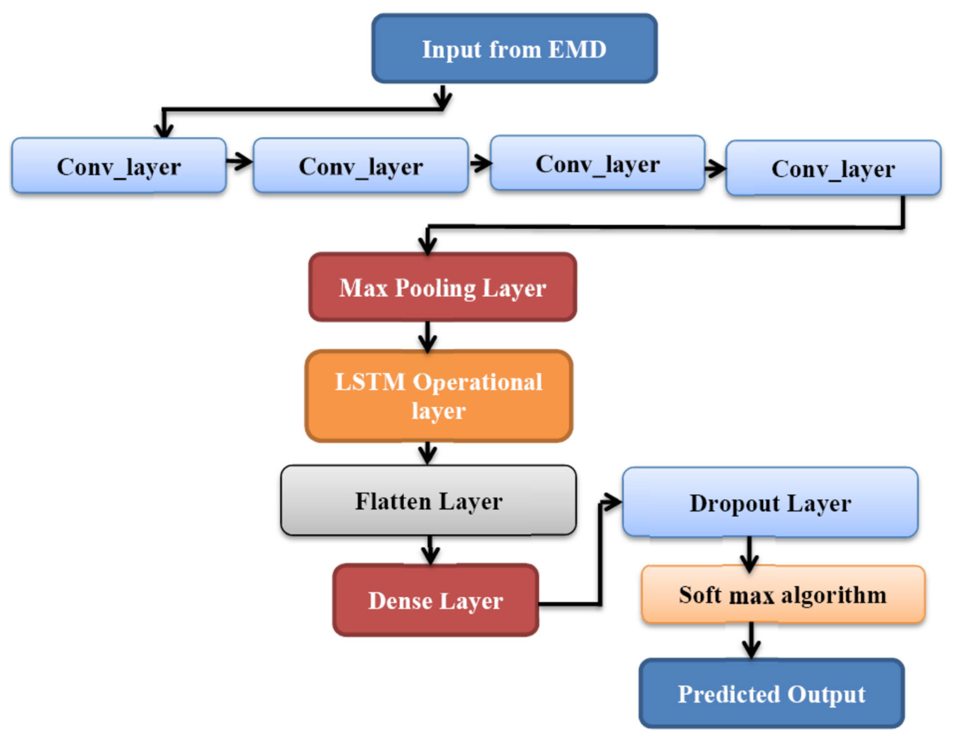
Figure 5 presents the developed DLSTM neural network in this research study for EV charging demand forecasts.
This research study attempts to perform a prediction of charging demand in respect of electric vehicles; the charging time in respect of the electric vehicles are important, and here, the output of the convolutional layer exceeds the input. This is avoided by padding the input data with zeros, and hence the output from the respective convolutional layers shall be identical and perform the deep layer training. The convolutional layer of the proposed DLSTM neural model extracts the significant time series features from the decomposed sub-series signals from EMD and passes the extracted EV charging features to the max-pooling layer of the predictor model. The DLSTM model proposed in this research study is modeled with convolutional layers, pooling layer, dense layer, LSTM layer, dropout layer and, finally, soft_max for presenting the output of the predictor model. In the new DLSTM predictor model, the convolutional operation is carried out for the input-to-state transition and for the state-to-state transition. The equations modified for the new deep learning based DLSTM model is derived as,
In Equation (14), ‘°’ represents the convolutional operator and * indicates the element-wise operator. The corresponding gates of the DLSTM model are defined by state variable at time t, kgt, ggt and Rgt that combines with the cell output.
The structure of the DLSTM model is designed with four convolutional layers with 30 neurons and a kernel size of four and for non-linear transformations the ReLU (rectified linear unit) is built with these convolutional layers. The output of the convolutional layer is a matrix of
U50×30, as there are 30 convolutional filters placed. The output matrix of the convolutional layer contains the weight of one filter and at the end of the fourth convolutional layer, a single dimension max pooling layer (pool size −2) exist and attains the output
U25×30. An LSTM operational layer follows the max pooling layer with 70 neurons, and here, there is a 30% recurrent dropout probability and a vector of
U1×70 is computed. Finally, a fully connected network with 70 neurons is formed with linear activations and then the final soft-max layer acts as the predictor. The EMD–AOA based DLSTM model evaluates the mean square error value along with the recurrent drop out, which facilitates in circumventing the over-fitting occurrences.For the modeled novel DLSTM, its encoder activation function ‘
Gencode’ and the labeled sample data points ‘
Xdata’ formulates the encode matrix as,
From the DLSTM, the reconstructed time-series data output is given by,
The designed deep learning layers with auto-encoder and decoder adapts to minimize the error criterion and achieve better prediction metrics during reconstruction operation. The loss function of the new DLSTM is given by,
During the deep learning process, the presence of non-linearity is evaluated using,
In Equation (18), ‘
gf_encode’ and ‘
gf_decode’ specifies the encoder and decoder activation function of the deep learning predictor model, ‘
W0′ represents the bias element and the weight matrices are ‘
Wx’ and ‘
’. The error is evaluated during deep training process using,
For all the deep LSTM layers, the encoder vectors are evaluated using,
The final predicted output from the DLSTM neural model is,
In Equation (21), ‘
GencodeN+1′ represents the trained values at the LSTM output layer and the new weights based on the gradients are evaluated to be,
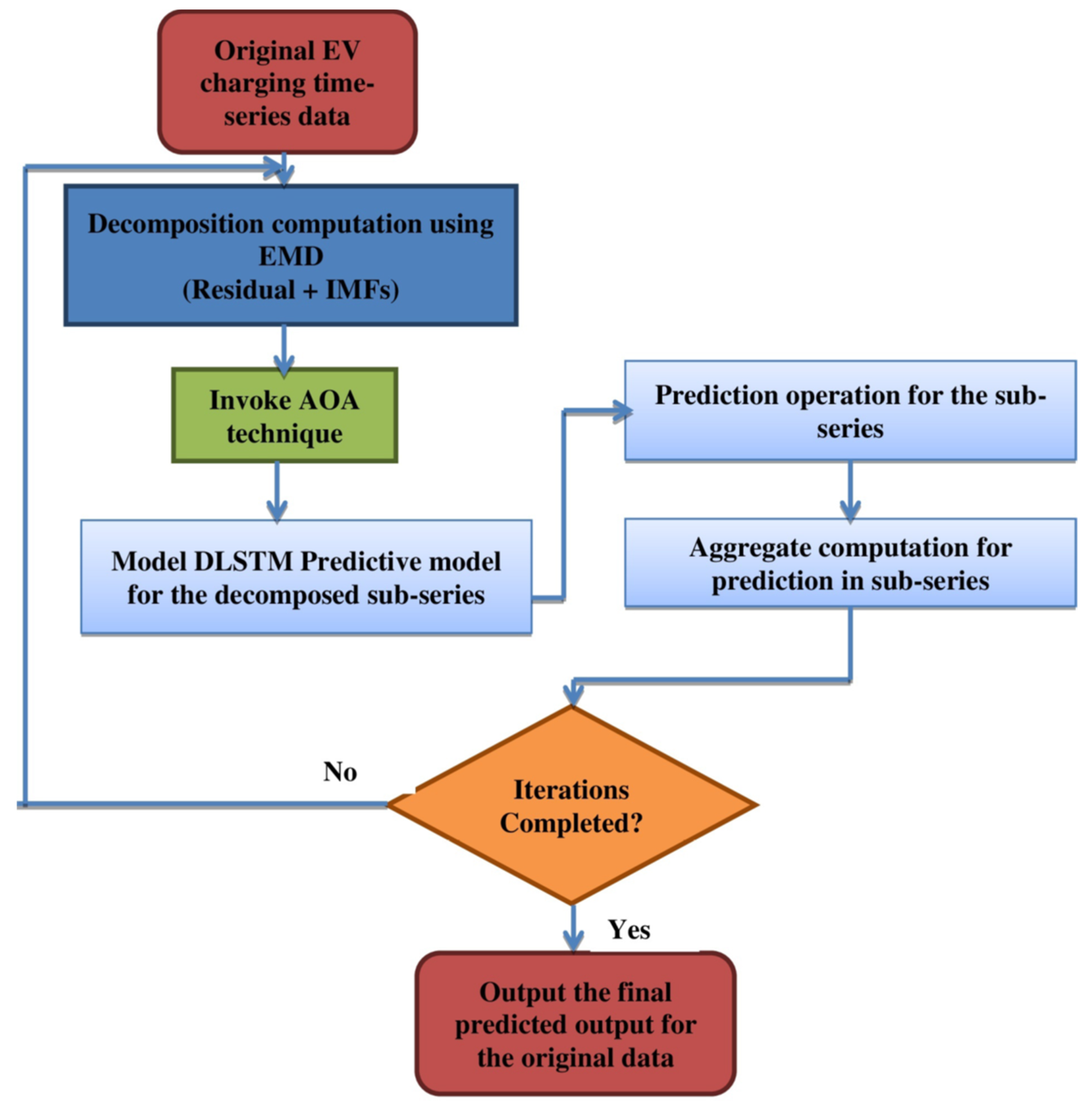
Figure 6 illustrates the complete process flow of the proposed EMD–AOA–DLSTM neural predictor model. The approach AOA tunes to obtain the optimized weight and bias component to be presented as initial values during the deep learning LSTM training. The above steps are repeated for the proposed DLSTM predictor model until the error value comes to the most possible minimal value. In respect of the evaluated predicted output and the original data, the mean square error metric is evaluated with,
Finally, the weights are updated during training and the predicted output corresponds to the point of attaining minimized MSE prediction value.
3.5. EV Charging Datasets
The dataset employed for testing and validating the proposed DLSTM predictor model pertains to the usage of electric vehicles within the campus of Georgia Tech, Atlanta, USA and the vehicles were charged at the conference center parking station and around 150 vehicles were flying around the campus [
63]. The average driving distance of the vehicles is 31 km.
Figure 7 provides the histogram plot of the duration of charging and a probability distribution curve.
Table 3 provides the sample electric vehicle charging datasets used in this research study. From the datasets, the input variables include Charging Time (hh:mm:ss), Energy (kWh), Greenhouse Gas (GHG) savings (kg), Gasoline savings (gallons) and cost incurred (USD). The output variable corresponds to predicting the charging demand of energy (kWh). The proposed EMD–AOA–DLSTM model is designed and simulated to operate on this electric vehicle dataset for predicting its charging demand.
4. Results and Discussions
The developed novel EMD–AOA–DLSTM predictor model is tested for its superiority and effectiveness for prediction of electric vehicle charging energy demand for the charging stations at Georgia Tech, Atlanta, USA. A simulation process is carried out in MATLAB R2021a environment on an Intel dual core i5 processor of 8GB physical memory. For the original EV charging time-series data, empirical mode decomposition is applied and residual and other IMFs are extracted, the data gets decomposed and the sub-series data forms the input for the deep LSTM neural network model. The basic AOA algorithm gets invoked on completion of the first trial run of the prediction algorithm, and subsequently, the weight coefficients and bias entities of the DLSTM neural predictor are tuned for their optimal values and then the deep learning algorithm performs its training. Based on the data decomposition of the sub-series using EMD and tuned optimal coefficients computed from the AOA technique, the deep learning-based long-short term memory network attempts to locate the best possible forecast value for the EV charging energy demand metric.
Table 4 lists the parametric values used during the training process of the proposed EMD–AOA–DLSTM neural predictor.
The proposed EMD–AOA–DLSTM predictor is tested for its superiority based on the performance metrics as given—mean absolute error (
MAE), mean square error (
MSE), root mean square error (
RMSE) and accuracy of prediction (
Apre) and they are evaluated with the following equations,
In Equation (24), ‘
N’ represents the total number of data samples, ‘
Yactual’ represents the original EV charging farm data and ‘
Ypredicted’ is the predicted output obtained using the proposed predictor model.
Figure 8 shows the EMD decomposed sub-series output of the considered EV data samples and these sub-series data are presented as input to the DLSTM model.
Figure 9 presents the design of the proposed DLSTM predictor model in the deep network designer of the MATLAB environment and simulation results are attained henceforth by training the predictive model created.
The decomposed sub signals, in respect of the EV charging datasets, are presented to the deep learning based long-short term memory neural network model. The deep LSTM is designed in the network designer with input layer of five neurons (charging time, energy, GHG savings, gasoline, and fee), nine deep dense layers and one output layer with single output neuron for the prediction of charging energy. At the initial iteration, the weights and bias coefficients are set to small random values and during the iterative learning process they are tuned for their optimal values using the AOA optimization process. The weights and bias will form the number of populations and the hierarchy of D, M, S and A will be adopted along with the position update of moa to attain the better optimal solutions, and subsequently deep learning progresses. Reaching the minimal mean square error value is the convergence point for the proposed predictive algorithm for the considered EV charging plant datasets.
The simulation process is done for the EV charging station datasets, the predicted EV charging energy (kWh) is computed using the decomposed sub-series data from EMD and the values of
MAE,
MSE,
RMSE and
Apre are evaluated and listed in
Table 5.
Figure 10 shows the plots of the predicted charging energy level with that of the actual charging energy level of the EV charging station. It is clear from
Figure 10 that the predicted EV charging energy is on par with the original charging energy level for the EV charging station.
Figure 11 depicts the convergence curve attained during the deep learning process of the proposed predictor model. At the time of training, the convergence was obtained at 251st epoch with an
MSE of 4.25516 × 10
−10 and for testing and validation the evaluated
MSE value is 5.96333 × 10
−10 and 5.5317 × 10
−10,respectively. The prediction accuracy attained during the convergence of the DLSTM predictor model is 97.14% with a minimal
MSE and an
MAE of 0.1083.
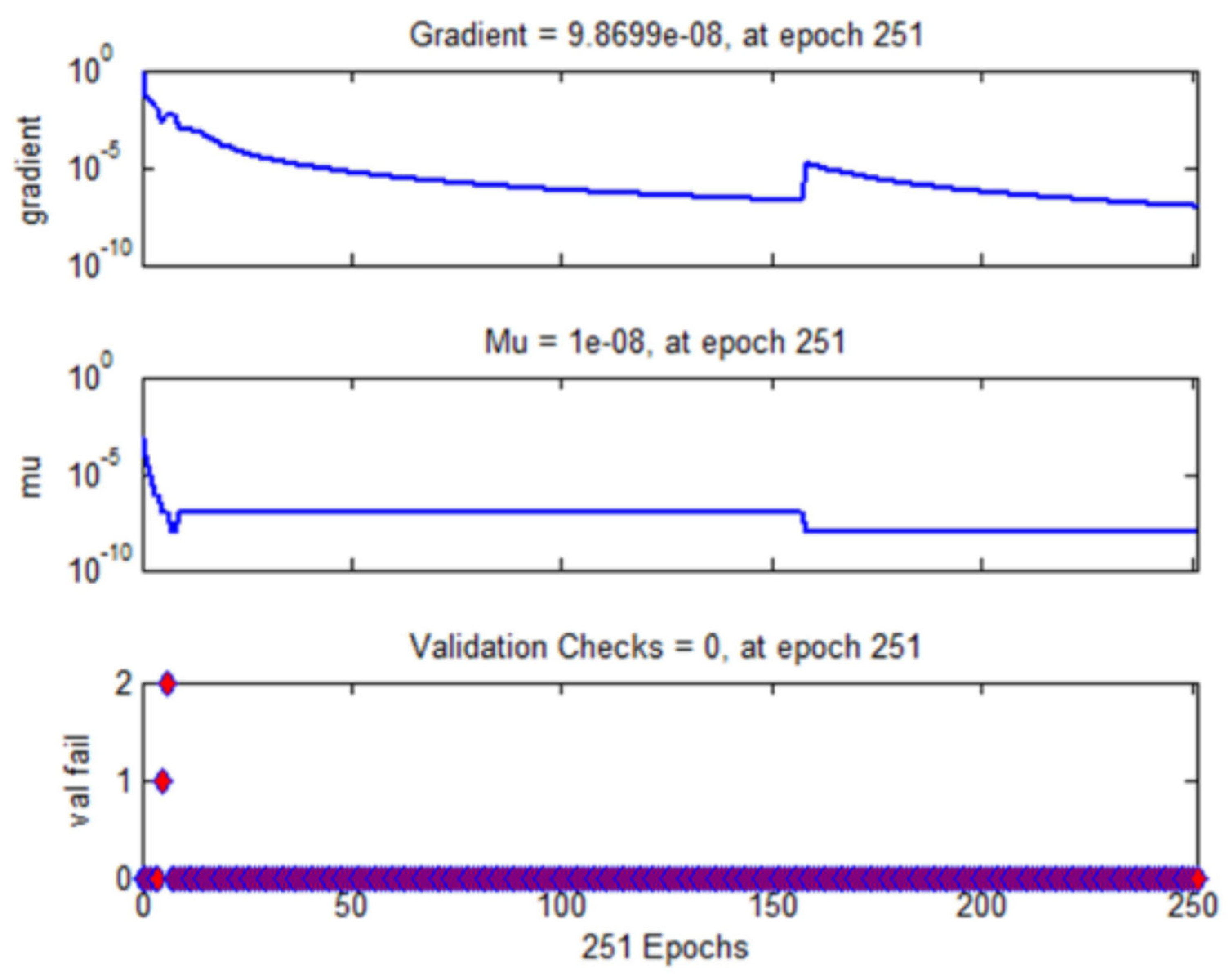
Figure 12 presents the variation in the gradient value, the momentum factor (Mu) and the validation fail checks carried out at the convergence point of 251st epoch. The plot confirms that a minimal value of gradient is obtained proving the efficacy of the developed predictor model. The regression plot at the time of prediction confirms that the value of regression coefficient R = 1 for training, testing and validating proving the validity and applicability of the proposed EMD–AOA–DLSTM predictor model. This figure has three metrics for a better understanding of the proposed EMD–AOA–DLSTM predictor model. The Gradient during the training process ranges in the limit between 0 to 10
−10. This indicates that the proposed predictor model will be able to improve its learning phase only when there is a small change in its weights and bias. This is well supported by the plot shown in
Figure 11.
Similarly, in the second part of the
Figure 12, the momentum factor (Mu) is plotted for the convergence point of 251st epoch. It may be observed from this plot that when the training epoch numbers increases, the momentum factor starts decreasing. Thus, establishing the proposed predictor model learning process is intact. The third part of
Figure 12 is the validation check plot. Which confirms the proposed predictor model is not trapped in a local minima. The all zero plot justifies that the network parameters adopted in this proposed predictor model is optimally chosen. Thus, with the evidence of all these three plots shown in
Figure 12, the proposed EMD–AOA–DLSTM predictor model demonstrates itself as a robust predictor model.
Figure 13 shows the regression plots obtained during the progressive training of the deep learning predictor. A good regression plot is the one where the predicted output value should be close to the target output value; thereby, the regression value R = 1. Thus, the proposed EMD–AOA–DLSTM predictor model again establishes itself as a robust predictor model.
The values of gradient value, the momentum factor (Mu),
MSE and the performance during the training process is presented in
Figure 14.
MSE values computed with respect to the number of iterations elapsed during the training and testing process is provided in
Table 6 for the EV charging station datasets. The convergence occurred by obtaining an
MSE value of 4.25516 × 10
−10 elapsed at 251st epoch for training process and during testing process, the
MSE was 5.96333 × 10
−10 at 251st for testing process.
Table 7 provides the sample of predicted EV charging demand value with that of the actual EV charging demand value at the Georgia Tech charging outlet. The predicted values prove their values are on par and near equal to that of the actual EV charging energy (kWh) for the considered charging station dataset. At the 251st Epoch, it has reached the convergence and attained the minimal
MSE value.
Employing the developed novel EMD–AOA–DLSTM predictor model, better prediction accuracy with minimized error values has been evaluated. The superiority of the predictor lies in its ability to carry out prediction process based on the memory states of the recurrent LSTM model. The new DLSTM model retains the information of the previous past, present, and thereby, considering the memory states, predicts the future value.
Deep learning procedure incorporated with the LSTM neural model intends to extract the significant features from the data through the convolutional layers and processing with sigmoidal functions takes place at the fully connected dense layers. This enables the proposed predictor to forecast the charging energy level for the future demand based on the previous history of electric vehicles and their charging energy levels. Furthermore, applying the classis arithmetic optimizer algorithm the optimal weight and bias coefficients are tuned and this helps the DLSTM predictor to overcome the over-fitting occurrences. A 4-fold cross validation is carried out on the EV datasets for training, testing and validating with the EMD–AOA–DLSTM predictor model and the results are computed during the simulation process.
5. Comparative Analysis
The novel predictor neural model proposed and simulated in this research study performed the prediction of charging demand energy level of the electric vehicles [
64,
65,
66]. The charging demand was predicted with respect to the charging time taken, charging energy in kWh, greenhouse emission savings, gasoline and the cost incurred for saving. With respect to the EV charging station considered in this research study, the EMD–AOA–DLSTM model resulted in better prediction accuracy and minimal mean square error during both training and testing process.
Table 8 provides a comparative analysis of the developed EMD–AOA based deep LSTM predictor with that of the earlier prediction techniques from existing works [
1,
10,
13,
16,
22,
24,
27,
50,
52]. The same Georgia Tech EV datasets were presented as input to all the comparison models for the respective codes in github.com and their comparison metrics—
MSE, training efficiency, testing efficiency, computational time and prediction accuracy was evaluated. It is clear from
Table 8 that the novel EMD–AOA–DLSTM model with
MSE of 4.25516 × 10
−10 and prediction accuracy of 97.14% has proved its superiority than other previous techniques from earlier works. The proposed model incurred a minimized computational time of 7.4 s than the Bayesian ELM model, which incurred 16.14 s [
1]. The average training and testing efficiency of proposed predictor was 98.62% and 98.03%, better than other compared models proving the efficacy of deep learning mechanism.TheEMD based sub-series decomposition and the AOA presence to attain optimal training parameters has enhanced the proposed DLSTM model to achieve predicted charging energy demand on par with that of the actual EV charging energy level.
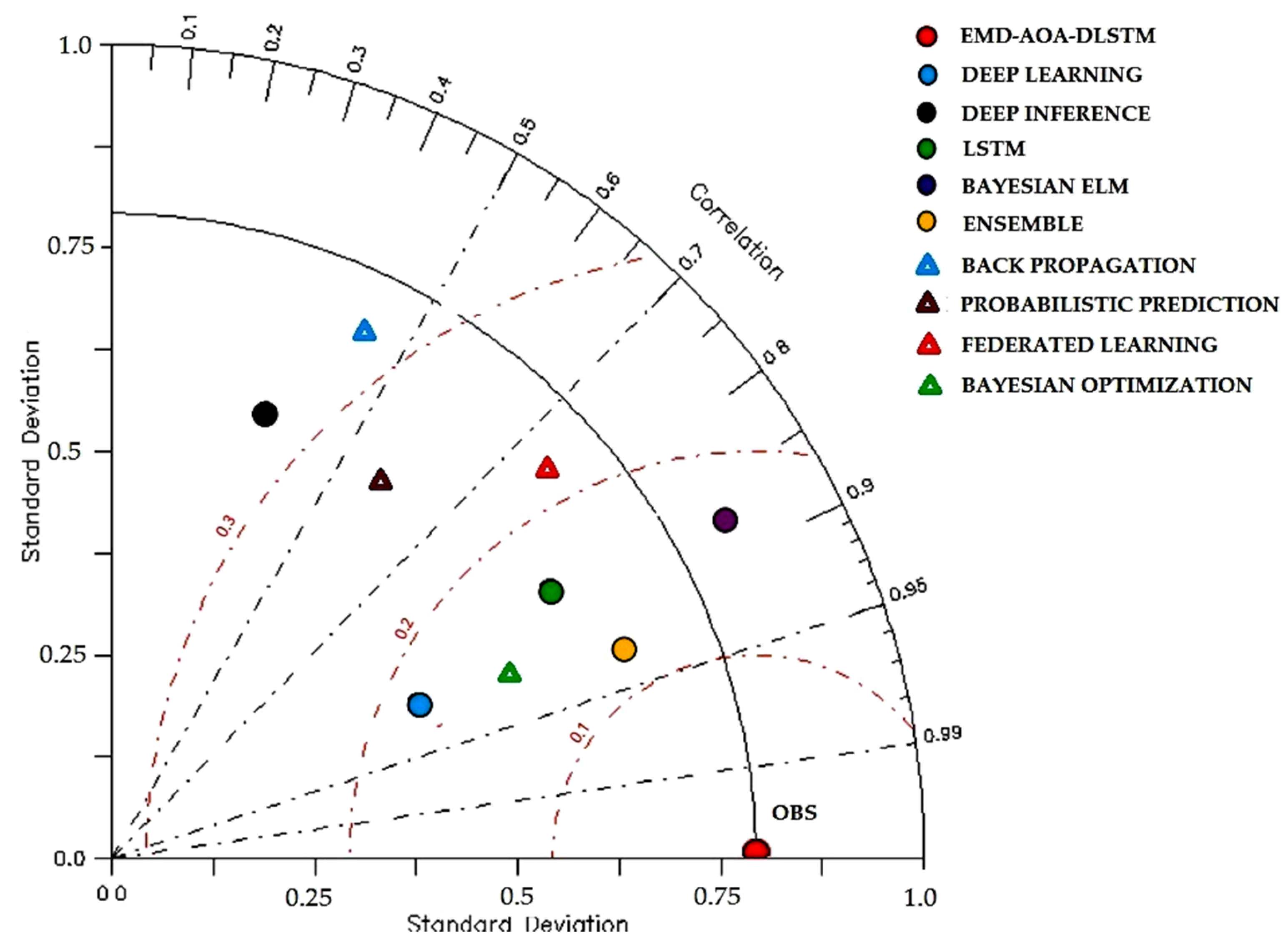
The Taylor diagram is another option to graphically summarize the proximity between the trained and tested data. The similarity between the two datasets is quantified in terms of their correlation, their root mean square error and the standard deviations. The Taylor diagram is widely used to understand the performance of various complex models used for prediction. Any model which has relatively high correlation and low RMSE will be marked as OBS in the X-axis of the Taylor diagram. The RMSE calculated using Equation (24) and the correlation value are used to arrive at the observed (OBS) value. The standard deviation of the test data can be related to the radial distance from the origin of the plot.
Here, amongst the ten well established models tabulated in
Table 8, all the prediction models, including the one proposed in this paper, are plotted in the Taylor diagram shown in
Figure 15. The position of the colored dots establishes the closeness of the models’ efficiency in predicting the test data using the trained data. The OBS value as per the diagram is 0.81.
It may be inferred from
Figure 15 that any model which has high correlation and low
RMSE will be declared as the successful prediction model. Accordingly, both the Bayesian ELM model (violet dot) and the probabilistic prediction model (brown triangle) has high
RMSE, but low correlation. Similarly, the federated learning (red triangle) model has a better
RMSE and correlation. It was followed by the ensemble learning model (yellow dot) followed by the LSTM model (green dot) and the Bayesian optimization (green triangle). As far as the deep inference framework (black dot) and back propagation (blue triangle) are concerned, both have performed very poorly in establishing both correlation and
RMSE. The deep learning (blue dot) model performed reasonably. Finally, the proposed EMD–AOA–DLSTM predictor (red dot) is demonstrated for its superiority based on the performance metrics by achieving relatively high correlation and low
RMSE, as depicted in the Taylor diagram.
Another widely adopted statistical plot to establish the comparison of prediction errors of various prediction models is shown in
Figure 16. The box plots are comprised of five components to portray the error statistics, namely, the three quartiles (lower, median and upper), and minimum and maximum error values. Accordingly, the box plot is shown here, such that the rectangle box conveys the range in which the prediction error is attained by the prediction models. The black lines show the median absolute error and the + signs conveys the prediction error outliers.
Another widely adopted statistical plot to establish the comparison of prediction errors of various prediction models is shown in
Figure 16. The normalized
RMSE is plotted for all the prediction models listed in
Table 8, including the proposed EMD–AOA–DLSTM prediction model. The box plots are comprised of five components to portray the error statistics. Accordingly, the box plot is shown here, such that the box conveys the range in which the prediction error is attained by the prediction models. The black lines show the median absolute error and the + signs conveys the prediction error outliers. For clarity in the figure, the different predictor models are abbreviated as follows: EAD: EMD–AOA–DLSTM; FEL: federated learning approach; ENS: ensemble learning; BOP: Bayesian optimization with ML; LST: LSTM model; BP: back propagation model; DPI: deep inference framework; DPL: deep learning model; BEL: Bayesian ELM neural model.
From the box plot it is clear that the proposed EMD–AOA–DLSTM predictor has the narrowest error range; on the contrary, the BP has the widest error range. In addition, the outliers and median error for the proposed model is also almost small compared to other predictor models. The DPL and DPI models almost produced the same error statistics. Similarly, BOP and ENS performed very much the same. BEL, LST, FEL and BP are very poor in reducing errors as well as in predicting the test data.
As the proposed deep LSTM neural model has a random initialization of weights, it is highly important to statistically validate the developed predictor model. In this study, two statistical parameters coefficient of determination and correlation coefficient are evaluated for the proposed neural model. When the values of both of these coefficients are nearer to 1, this confirms the statistical validity of the proposed neural network model.
Table 9 shows the evaluated values of the statistical parameters. From the table, it is clear that both of these values are closer to 1, proving that the proposed model is statistically valid.


