Article

Analysis of the Working Response Mechanism of Wrapped Face Reinforced Soil Retaining Wall under Strong Vibration

1
Key Laboratory of Earthquake Engineering and Engineering Vibration, Institute of Engineering Mechanics, China Earthquake Administration, Harbin 150080, China
2
College of Geological Engineering, Institute of Disaster Prevention, Sanhe 065201, China
3
Hebei Key Laboratory of Earthquake Disaster Prevention and Risk Assessment, Sanhe 065201, China
4
Key Laboratory of Building Collapse Mechanism and Disaster Prevention, China Earthquake Administration, Sanhe 065201, China
*
Author to whom correspondence should be addressed.
Sustainability 2022, 14(15), 9741; https://doi.org/10.3390/su14159741
Submission received: 4 July 2022 / Revised: 30 July 2022 / Accepted: 2 August 2022 / Published: 8 August 2022

Abstract

:
A series of shaking table tests were carried out to explore the dynamic characteristics and working mechanisms of wrapped-face reinforced soil-retaining walls under strong vibration. Under the 0.1–1.0 g horizontal peak ground acceleration (HPGA), the damping ratio of sand shows a downward trend as a whole, so the acceleration amplification coefficient decreases with the increase of HPGA. However, when HPGA reaches 1.0 g, the acceleration amplification coefficient increases; the range of acceleration amplification coefficient at the top of the wall is 1.69–1.36. When HPGA is 1.0 g, the maximum cumulative residual displacement of the panel is 2.96% H, and the maximum uneven settlement of the sand is 3.57% H, both of which have exceeded the limit of the specification. With the increase of HPGA, the ratio of the dynamic earth force increment to the total dynamic earth force gradually approaches 50%. Since the reinforcement effect of geogrid is not considered, the predicted value of traditional earth pressure theory is different from the measured value. According to the Washington State Department of Transportation displacement index, the deformation range of wrapped-face reinforced soil-retaining walls is divided into three stages: the quasi-elastic stage, the plastic stage, and the failure stage.

1. Introduction

The wrapped-face reinforced soil-retaining wall is a kind of flexible panel retaining wall composed of geosynthetics back-packed with geobag inclusions. By sowing grass seeds in the geobag to form a green landscape panel, the total carbon emission of the structure in the whole life cycle is negative [1], which responds to the current strategic goal of carbon neutrality. At present, this structure is widely used in many fields such as in highways [2], railways [3,4], embankments [5], and substations [6]. During the 2011 Tohoku earthquake (off the pacific coast), the appearance and performance of a wrapped-face reinforced soil-retaining wall in the Miyagi prefecture were not affected (Figure 1) [7], which preliminarily proved that the seismic performance of the structure was superior.
The stiffness of the wrapped-face reinforced soil-retaining wall is less than that of the rigid panel retaining wall, and its strong deformation coordination ability allows the panel to produce partial deformation in the construction stage, making it difficult to ensure the compactness of the backfill behind the panel. In the seismic design, the design method of the rigid panel reinforced earth-retaining wall is still used, Therefore, it is necessary to study the seismic failure mechanism of such retaining walls.
Many scholars have conducted in-depth studies on the seismic performance of the wrapped -ace reinforced soil-retaining wall. Krishna [8,9] studied the influence of fill compactness on the seismic dynamic response of wrapped-face reinforced soil-retaining walls under different excitation load frequencies. Sakaguchi [10] studied the dynamic characteristics of the wrapped-face reinforced soil-retaining wall and the influence of different factors on the horizontal displacement of the retaining wall, and proposed a calculation method of horizontal displacement considering seismic effect. Ramakrishnan [11] deduced a critical acceleration analysis method and found that the critical acceleration of the wrapped-face reinforced soil-retaining wall as a flexible panel retaining wall was only half of that of the rigid panel retaining wall. However, when the peak acceleration of local vibration was less than 0.5 g, the wrapped-face reinforced soil-retaining wall could play a sufficient role without damage. Huang [12] calculated the dynamic earth pressure increment distribution of the retaining wall in the model test by the tensile force of the reinforcement. The results show that the lateral earth pressure distribution of the wrapped-face reinforced soil-retaining wall is irregular trapezoidal along the height of the wall, under earthquake action. Roessing [13,14] did not observe the obvious failure surface of the backfill during the test and suggested that the deformation of the wrapped-face reinforced soil-retaining wall was related to the density of the backfill, the stiffness and spacing of the reinforcement, and the slope of the wall. Yang [15] explored the amplification effect of the wrapped-face reinforced soil-retaining wall acceleration, and believed that the horizontal acceleration inside the retaining wall showed an uneven distribution law with the increase of the retaining wall height, and changed with the change of the input acceleration. Zhu [16] suggested that the peak dynamic earth pressure distribution of the wrapped-face reinforced soil-retaining wall and rigid panel reinforced soil-retaining wall under an earthquake was the opposite. Duan [17] used the quasi-static method to calculate the internal and external stability coefficient of the wrapped-face reinforced soil-retaining wall and compared it with the theoretical value. Model tests and details of the dynamic characteristics of wrapped-face reinforced soil-retaining wall are summarized in Table 1.
The shaking table test has been carried out to study the deformation mode, horizontal displacement calculation method, and soil pressure distribution of the wrapped-face reinforced soil-retaining wall, but there are still some problems that have not been discussed. For example, the deformation and failure stage of the wrapped-face reinforced soil-retaining wall under an earthquake is not clear, which hinders the development of the performance-based seismic design method [18]. The acceleration amplification coefficient in some specifications is not consistent with the actual situation [19], which is crucial in seismic design. In addition, it is necessary to study the natural frequency and damping [20,21] of wrapped-face reinforced soil-retaining walls to explore the dynamic characteristics. Focusing on these problems, the dynamic response analysis of the wrapped-face reinforced soil-retaining wall under strong vibration was carried out. According to the acceleration amplification effect and the dynamic characteristics, the seismic working mechanism was revealed. Based on the horizontal residual displacement, the deformation stages are divided, which provides references for the seismic design of wrapped-face reinforced soil-retaining walls.
Table 1. Summary of dynamic model test of wrapped face reinforced soil retaining wall.
ReferenceTest Type aHeight ModelLength to Height RatioInput
Motion b
ReinforcementAmax c
Krishna [8,9]ST0.60 m1.25Sine.geotextile0.2 g
Sakaguchi [10]ST1.50 m2.30Sine.geogrid0.72 g
Sakaguchi [10]CST0.15 m2.30Sine.geotextile12 g
Ramakrishnan [11]ST0.81 m2.50Sine.geotextile0.6 g
Huang [12]ST0.60 m1.40Sine.geotextile1.72 g
Roessing [13,14]CST0.38 m1.60EQgeotextile/metallic strips1.0 g
Yang [15]CST0.16 m1.20Sine.geotextile1.0 g
Zhu [16]ST1.60 m1.56EQgeogrid0.616 g
Duan [17]ST2.00 m1.40EQgeogrid0.616 g
Sabermahani [22]ST1.00 m-Sine.geotextile/geogrid0.3 g
a: ST = Shaking table test, CST = Centrifuge shaking table test. b: Sine. = sinusoid, EQ = scaled earthquake. c: Amax = peak acceleration, g = acceleration of gravity. The backfill behind the panel is inviscid soil in all tests.

2. Shaking Table Model Test

The test was carried out on a three-dimensional and six-degree-of-freedom electromagnetic vibration table in the Key Laboratory of Building Collapse Mechanism and Disaster Prevention, China Earthquake Administration, Institute of Disaster Prevention. The maximum horizontal acceleration of the system was ±2.0 g. The maximum effective load was 1.5 t; the maximum horizontal travel was ±10 cm. The rigid model box used in the test was 1.5 m × 0.5 m × 1.2 m (length × width × height). In order to reduce the influence of boundary conditions on the test results, vaseline was smeared on the side wall of the model box to reduce the friction between the side wall and the model, and an 8 cm thick sponge was placed on the back wall of the vibration direction of the model box to reduce the reflection of the wave [20,23]. At the same time, the sensor was arranged along the center line of the width direction of the model to minimize the boundary constraints on the model.

2.1. Similitude Laws

In order to ensure the test model truly reflected the response law of prototype engineering under earthquake action, and comprehensively consider the size and performance of the test device, the design similarity ratio was defined as 1:3, which is used to simulate the prototype retaining wall with a height of 3 m. The similarity relationship used in the test is shown in Table 2.

2.2. Model Design

The size of the test model and the location of the sensor are shown in Figure 2. The model is 1 m in length, 0.5 m in width, and 1 m in height. It is composed of five reinforcement layers and the reinforcement spacing is 0.2 m. The horizontal LVDT (Linear Variable Differential Transformer) is arranged at the center of each reinforcement layer to monitor the horizontal displacement of each reinforcement layer during an earthquake. At the top of the model from 0 cm, 35 cm, 70 cm, and 80 cm away from the panel, the vertical LVDT is set to monitor the vertical settlement of the reinforced area and the non-reinforced area during the earthquake. Horizontal accelerometers are arranged behind the panel of each layer and in the reinforcement area to record the acceleration response at each position of each layer during the earthquake. Earth pressure cells are arranged behind the panel of each layer to record static and dynamic earth pressure behind the panel; and fixed strain gauge on geogrid 1 cm away from the panel to monitor strain increment during vibration. In addition, the acceleration is set on the shaking table to record the input ground motion time history of the test model.

2.3. Backfill Material

The backfill used in the test model was medium sand, the gradation curve of the sand is shown in Figure 3. A series of geotechnical tests were carried out to measure the following physical and mechanical properties of sand: the coefficient of uniformity Cu = 2.055, the curvature coefficient Cc = 1.262, the internal friction angle φ = 41°, and the specific gravity Gs = 2.86. The maximum dry density was 1.99 g/cm3 and the minimum dry density was 1.52 g/cm3. According to the Unified Soil Classification System (USCS), the sand used in this paper is classified as poorly graded sand (SP). In the process of model construction, each 100 mm thick sand layer was compacted once. By controlling the quality of each layer of sand, the relative density of sand was controlled to Dr = 0.7, and the corresponding sand density was 1.82 g/cm3.

2.4. Reinforcement

The geogrid used in the test is EG50R unidirectional high-density polyethylene (HDPE) geogrid. According to ASTM D6637 [24], the tensile strength T2% of the geogrid under 2% strain is 17.4 kN/m and the ultimate tensile strength, Tult = 57.9 kN/m, was measured by MTS electro-hydraulic servo universal testing machine. Due to the limitation of material types, it is impossible to strictly scale the geogrid according to the similarity ratio design. Therefore, the mechanical properties of materials were used as the key points of similarity design [25,26] to scale the materials. The geogrid was treated with rib removal at the similarity ratio of 1:3, and 2/3 of the geogrid longitudinal ribs were eliminated. The geogrids were horizontally arranged in the reinforcement area, and the reinforcement spacing was 0.2 m. The length of geogrid-reinforced section was 0.7 m.

2.5. Panel

Geogrid was used to back-pack geobag inclusions to form the panel of the retaining wall. The geobag is made of YG-M polypropylene by self-cutting and sewing. The transverse/longitudinal tensile strength is 1.1 kN/m, and the transverse/longitudinal elongation at break is 71%. The panel is lapped by the backpack geobag staggered joints. There are two sizes of geobags: the A-type geobag size is 0.25 m × 0.1 m × 0.1 m (length × width × height) and the B-type geobag size is 0.125 m × 0.1 m × 0.1 m (length × width × height). The sand in the geobag is completely consistent with the sand behind the panel.

2.6. Input Motions

The Wolong wave (referred to as WL wave) collected by NS to Wolong station during the Wenchuan earthquake, and the El Centro wave (referred to as El wave) collected by NS to El Centro station during the Imperial Valley earthquake in the United States were selected as the input ground motion time history. The ground motion time history with the similarity ratio of 1:3 after normalization is shown in Figure 4.
The time history of ground motion is input in the order of peak value, from small to large. After the end of each change in wave magnitude, white noise with a peak acceleration of 0.05 g is used to sweep frequency, and the change of natural vibration frequency after the earthquake is monitored. The test loading conditions are shown in Table 3.

3. Results

3.1. Model Damage Phenomena

In the process of model building, a thin layer of blue sand is laid every 10 cm, and the initial position of the blue sand as well as the position after the end of each working condition are recorded to facilitate the statistics of the settlement of each reinforced layer. Figure 5 is the seismic damage phenomenon of the retaining wall model after the end of the El wave 1.0 g working condition. It can be seen from the figure that the settlement of each reinforced layer was relatively uniform, and the panel had obvious displacement, but there was no sand leakage. As the panel moves outward, the settlement of sand behind the panel is obvious, which is also a common problem in retaining walls [15]. The deformation mode of retaining walls is a combination of base sliding and overturning [27], which is consistent with the phenomenon observed by Koseki [28].

3.2. Acceleration Response
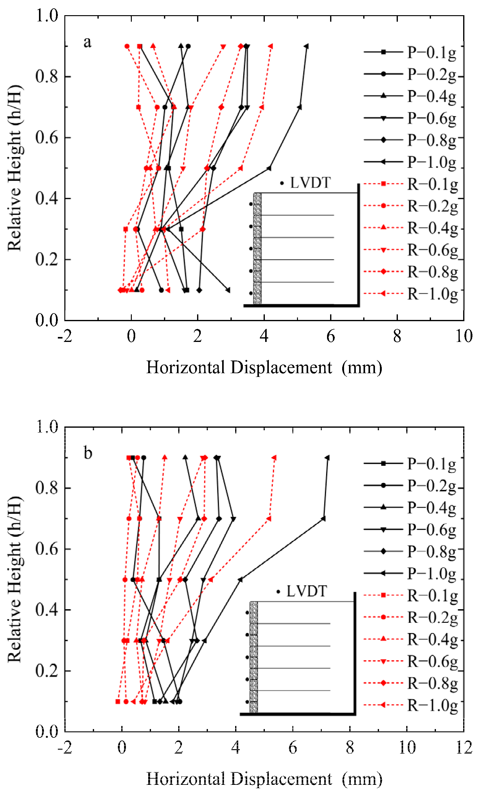
The ratio of the root mean square acceleration of each measuring point to the root mean square acceleration of the table surface is defined as the acceleration amplification factor. The calculation method for root mean square acceleration is shown in Equation (1).
a r m s 2 = 1 T d 0 T d a 2 ( t ) d t
Note: arms stands for root mean square acceleration; Td for vibration duration; a(t) for acceleration time histories.
Figure 6 shows the acceleration amplification coefficients behind the panel (referred to as S) and the reinforcement area (referred to as N) of the retaining wall model along the wall height. When the height is the same, the acceleration amplification coefficient at the panel is slightly smaller than that at the reinforcement area under the same working condition, and the percentage difference is between 0.35% and 2.08%. The acceleration distribution inside the retaining wall is relatively uniform. Therefore, the acceleration difference between the panel and the reinforcement area can be ignored in the seismic design.
The time-domain analysis of the model white noise sequence is carried out to obtain the first-order natural vibration frequency and damping ratio of the wrapped-face reinforced soil-retaining wall, as shown in Figure 7. Combined with Figure 6 and Figure 7, the acceleration amplification factor decreases first and then increases with the increase of the peak acceleration of the input ground motion due to the influence of the nonlinear characteristics of the soil; this phenomenon is consistent with the model results reported by Zhu [17]. The reason is that with the increase of the dynamic load level of the model, the natural vibration frequency of the retaining wall decreases, and the damping ratio increases, so that the seismic isolation effect of the sand is enhanced. This results in the acceleration amplification factor of the peak acceleration less than 1.0 g decreasing with the increase of the amplitude of the input ground motion. However, when the peak acceleration reaches 1.0 g, the acceleration amplification factor increases with the increase of input ground motion amplitude.
There are mainly two kinds of calculation methods for the design acceleration of retaining walls in the current specification. The first method does not consider the height. For example, AASHTO (American Association of State Highway and Transportation Officials, Washington, DC, USA), NCMA (National Concrete Masonry Association, Herndon, VA, USA), NCHRP (National Cooperative Highway Research Program, Washington, DC, USA), and other specifications use Equation (2) to calculate the design acceleration of retaining walls. The second method considers the wall height, FHWA (U.S. Department of Transportation Federal Highway Administration, Washington, DC, USA) uses Equation (3) to calculate the acceleration amplification coefficient of the retaining wall. The ‘Code for Seismic Design of Railway Engineering’ (Chinese Highway Specification) takes 12 m as the boundary to calculate the acceleration amplification coefficient, as shown in Equation (4). The ‘seismic code for highway engineering’ (Chinese Railway Specification) adopts Equation (5) to calculate the linear acceleration amplification factor.
A m = ( 1.45 A ) A
a = 1 + 0.01 H [ 0.5 ( F V S 1 A ) ] 1
Note: When the height of retaining wall is less than 20 feet (about 6.1 m) and the foundation condition is very strong, the acceleration amplification factor is about 1.
a = { 1 H 12 m 1 + h i H H > 12 m
a = { 1 3 h i H + 1.0 ( 0 h i 0.6 H ) 3 2 h i H + 0.3 ( 0.6 H < h i H )
Note: Am is the design acceleration; A is the peak acceleration; a for acceleration amplification factor; H is the height of retaining wall; FV is site coefficient; S1 is the spectral acceleration of period 1 s; hi for retaining wall toe to section i height.
It can be seen from Figure 6 that with the increase of layer height, the acceleration amplification coefficient shows a nonlinear increasing trend, and the maximum acceleration amplification coefficient occurs at the top of the retaining wall, reaching 1.69 times, indicating that with the increase of layer height, the seismic wave energy gradually gathers to the top of the wall. However, AASHTO, FHWA (less than 6.1 m), and the Chinese Railway Specification (less than 12 m) did not consider the distribution difference of acceleration amplification coefficient along the wall height, which was inconsistent with the actual situation [8,9,13,16].
The calculation method considering the height of retaining wall is compared with the measured acceleration amplification coefficient. It can be seen from Figure 5 that the trend of the Chinese Highway Specification value is consistent with the measured value, but the value is slightly conservative, especially at 0.6 H. That is, there is a certain error between the standard values and the test results, and the standard value needs to be corrected. For practical engineering, the design value can be calculated according to the measured results of the original size shaking table test when the test conditions and economic conditions are satisfied. If there is no condition for the original size test, the analogy method can be used for calculation, according to the results of the scaled model shaking table test. In this paper, according to the measured results of the shaking table test, the acceleration amplification coefficient distribution formula of the wrapped-face reinforced soil-retaining wall is summarized, as shown in Equation (6):
a = { 2 3 h i H + 1.0 ( 0 h i 0.6 H ) 3 4 h i H + 0.95 ( 0.6 H < h i H )
Note: a is for acceleration amplification factor; H is the height of retaining wall; hi for retaining wall toe to section i height.

3.3. Deformation

Figure 8 shows the distribution of horizontal peak displacement (referred to as P) and residual displacement (referred to as R) along the wall height. It can be seen from the figure that the peak dynamic displacement has a nonlinear relationship with the wall height and peak acceleration. The higher the wall height, the greater the peak acceleration, and the greater the peak dynamic displacement of the wall. When the peak acceleration ≤ 0.2 g, the maximum peak dynamic displacement does not exceed 0.2% H, which has little effect on the retaining wall. This verified Ramakrishnan’ s conclusion that the critical acceleration of the wrapped-face reinforced soil-retaining wall is 0.25 g [12]; when the peak acceleration is between 0.2 and 0.8 g, the maximum displacement occurs at 0.7 times the wall height; when the peak acceleration reaches 1.0 g, the maximum displacement occurs at the top of the wall, reaching 0.72% H.
The unrecovered part of the horizontal displacement of the retaining wall model after an earthquake is residual displacement, and excessive residual displacement will affect the safety of the retaining wall. The distribution of residual displacement in Figure 8 shows that when the peak acceleration is less than 0.2 g, the residual displacement at each position is close to 0, which is similar to a straight line; when the peak acceleration >0.2 g, the residual displacement increases with the increase of wall height and peak acceleration, and the maximum residual displacement basically occurs at the top of the wall. Under the condition of 1.0 g peak acceleration, the maximum residual displacement is 0.54% H (5.4 mm in this paper). Affected by the local deformation of the back-packed geotextile bags, the residual displacement distribution curve of the wrapped-face retaining wall is less smooth than that of the rigid panel retaining wall [29,30].
Since the horizontal displacement of the retaining wall is intuitive and easy to measure, displacement index is often used in the current specification and as a method to quickly determine the state of the retaining wall [31,32]. WSDOT uses 1.7% H residual displacement as the failure criterion for wrapped-face reinforced soil-retaining walls. The maximum cumulative residual displacement after each peak acceleration condition is summarized in Figure 9. When the peak acceleration condition of 1.0 g is over, the maximum cumulative residual displacement of the model is 2.96% H, which exceeds the WSDOT limit. The deformation range of the retaining wall is defined as three main stages: quasi-elastic stage, plastic stage, and failure stage. The quasi-elastic stage represents the non-permanent displacement or the lateral displacement that can be ignored with small values. The failure stage is that the maximum residual displacement of the retaining wall exceeds the WSDOT specification value, and the plastic stage is located between the first two. It can be seen from Figure 7 that when the peak acceleration is between 0.6 g and 0.8 g, the damping ratio of the sand in the test model decreases. Combined with Figure 7 and Figure 9, the critical failure acceleration of the test model of the wrapped-face reinforced soil-retaining wall is determined to be 0.71 g.
During the vibration process, the top settlement is formed by repeated cycles of loading and unloading. The cumulative residual settlement after each peak acceleration condition is shown in Figure 10. When the peak acceleration is less than 0.4 g, the settlement behind the panel is small. With the increase of peak acceleration, the cumulative settlement value gradually increases. When the peak acceleration is greater than 0.4 g, the settlement behind the p is arranged in a ‘n’ shape, that is, the settlement of the unreinforced area is the largest, followed by the back-packed panel and the end of the reinforced area, while the settlement value in the middle of the reinforced area is the smallest. The reason for the large settlement value after the back-packed panel is that the sand is redistributed during the forward tilt of the back-packed panel, so the settlement is caused. Under the peak acceleration conditions of 0.8 g and 1.0 g, the maximum uneven settlement reached 2.07% H and 3.57% H, respectively, exceeding the 2% H limit of AASHTO specification; after the end of all working conditions, the maximum settlement value of the model occurred in the unreinforced area, and the maximum value was 4.83% H. According to the cumulative permanent displacement value and cumulative residual settlement value, the volume of the post-earthquake model was 98.59% of that before the earthquake, and the change range is small. Therefore, it is not necessary to consider the change of packing density in seismic design.

3.4. Earth Pressure

The active earth pressure generated in the vibration process is the main reason for the displacement of the wall [33,34]. The Mononobe-Okabe method (referred to as M-O method) and Seed-Whiteman method (referred to as S-W method) are used to calculate the total dynamic earth force in various specifications of the industry. Seismic earth pressure is calculated based on the M-O method in Chinese Railway Specification, Japanese Code for Design of Railway Structures, New Zealand Bridge Handbook, FHWA, AASHTO, NCMA and EU8 Codes, as shown in Equation (7). The S-W method is used to calculate the seismic earth pressure in the Chinese Highway Specification, as shown in Equation (8).
{ P A E = 1 2 γ H 2 K A E K A E = c o s 2 ( φ θ ) c o s θ c o s ( δ + θ ) [ 1 + sin ( φ + δ ) sin ( φ θ ) cos ( δ + θ ) ] 2 K dyn = c o s 2 ( φ θ ) cos θ cos ( δ + θ ) [ 1 + sin ( φ + δ ) sin ( φ θ ) cos ( δ + θ ) ] 2 c o s 2 φ cos δ [ 1 + sin ( φ + δ ) sin φ cos δ ] 2
{ P A E = P S + Δ P d y n P S = 1 2 γ H 2 K a Δ P d y n = 1 2 γ H 2 K d y n K a = c o s 2 ( φ α ) c o s 2 α cos ( δ + α ) [ 1 + sin ( φ + δ ) sin φ cos ( δ + α ) ] 2 K d y n = 3 4 k h
Note: PAE is total dynamic earth force; γ is the sand weight; H is the wall height; KAE is seismic earth pressure coefficient; PS is static earth pressure; ΔPdyn is dynamic earth force increment; Ka is the static earth pressure coefficient; Kdyn is the dynamic increment active earth pressured coefficient; kh is the horizontal seismic coefficient; φ is the internal friction angle of sand; θ is the seismic inertia angle; δ is the soil-wall interface friction angle; α is the wall-back inclination.
The total dynamic earth pressure monitored in the test is converted into total dynamic earth force by using the area moment method, through this process, the height of resultant force action point can be obtained. The comparison between the measured total dynamic earth force and the two calculation methods is shown in Figure 11. The total dynamic earth force under different ground motion time histories has little difference, and the maximum value can reach 10.68 kN/m. The predicted distribution trend of the S-W method is consistent with the measured value, but the former value is slightly smaller than the latter, and there is a certain risk in seismic design. Limited by the seismic inertia angle θ and the internal friction angle φ, the M-O method can only calculate the total dynamic earth force before the 0.8 g working condition in this paper. When the peak acceleration is greater than 0.6 g, the predicted value of the M-O method is much larger than the measured value, therefore, the M-O method is not suitable for the calculation of seismic earth pressure in the peak acceleration region.
Each specification has different provisions regarding the normalized point of application for the resultant total dynamic earth force, and the AASHTO specification defines the position of resultant force point as H/3 away from the toe of the wall, which is the same as that of the M-O method. FHWA stipulates that the position of the resultant force action point is H/2 from the toe of the wall. NCMA believes that the position of the resultant force action point changes in the range of H/3~2 H/3, and the degree of change depends on the magnitude of the dynamic earth force increment. From Figure 11, it can be seen that the position of total dynamic earth force acting point changes between 0.30 H and 0.32 H from the toe of the wall, which is close to the recommended value of H/3 from the toe of the wall in the AASHTO specification.
The S-W method decomposes the total dynamic earth force into Coulomb active earth pressure and dynamic earth force increment. The retaining wall is in equilibrium under static action, therefore, the dynamic earth force increment is an important factor affecting the seismic safety of the retaining wall. The area moment method is used to convert the dynamic earth pressure increment collected by the earth pressure cell in the experiment into the dynamic earth force increment, in which the height of the resultant force point can be solved. The dynamic earth force increment is standardized (divided by 0.5γH2) to obtain the measured seismic earth pressure increment coefficient Kdyn. Figure 12 compares the measured values with the standard values, and the measured coefficient increases with the increase of peak acceleration. In the range of 1.0 g, the measured coefficient is always in the range of M-O method and S-W method, and the maximum measured value is 0.54. The distribution law of the S-W method coefficient is consistent with the measured value, and the value is slightly conservative, so it can be used as the upper limit. When the peak acceleration reaches 0.8 g, the M-O method will overestimate the dynamic increment active earth pressured coefficient. The S-W method considers that the normalized point of application for the resultant of the dynamic earth force increment acts on the height of 0.6 H, but the measured height is variable, with the increase of peak acceleration, the measured height gradually decreases from 0.63 H to close to H/3 height, which is consistent with the conclusion of Bathurst [35].
It can be seen from Figure 11 and Figure 12 that the traditional soil pressure theory cannot accurately predict the test results. Wilson also draws similar conclusions through the shaking table test [36], which is mainly because the theoretical method does not consider the reinforcement effect of geogrid.
The ratio of dynamic earth force increment to total dynamic earth force in Figure 13 shows that the measured percentage increases with the increase of peak acceleration, and the maximum measured percentage is 46.5%. However, when the peak acceleration is greater than 0.6 g, the percentage is no longer significantly increased, but more close to 50%. This is due to the fact that the retaining wall has entered the failure stage after the peak acceleration reaches the critical failure acceleration of 0.8 g and 1.0 g, and the deformation and energy dissipation characteristics of the panel release some seismic dynamic earth pressure during the vibration process. The distribution trends of S-W method and M-O method are close, and the values are greater than the measured values. When the peak acceleration is greater than 0.4 g, both methods believe that the dynamic earth force increment plays a leading role in the total dynamic earth force. The maximum proportion of M-O method is 89.6%, and that of S-W method is 79.6%, which are greatly different from the measured values.
The comparison of the distribution of the horizontal static earth pressure after the stability balance of the retaining wall, and after the earthquake in each working condition with the coulomb active earth pressure and the static earth pressure is summarized in Figure 14. From the two figures, it can be seen that the measured horizontal static earth pressure at the toe of the wall is much larger than the static earth pressure, and the maximum value is 16.97 kPa. The measured horizontal earth pressure at the top of the retaining wall is greater than the static earth pressure, which is caused by the forward deformation and extrusion of the retaining wall. After the stability balance of the retaining wall is completed, the horizontal earth pressure of the middle three layers is almost consistent with the Rankine active earth pressure. When the peak acceleration is less than or equal to 0.4 g, the horizontal static earth pressure behind the three-layer wall in the middle of the retaining wall decreases with the increase of the peak acceleration, which is consistent with the in-situ monitoring results of Chengdu-Kunming railway [37]. The reason for this is that the wall surface is inclined and the earth pressure behind the wall is released. When the peak acceleration is 0.6 g, the backfill behind the wall is squeezed forward under the action of seismic inertia force, so that the earth pressure behind the three-layer wall in the middle of the retaining wall is greater than the coulomb active earth pressure. When the peak acceleration is greater than 0.6 g, the earth pressure behind the three-layer wall in the middle of the retaining wall is greater than the static earth pressure, the maximum value is 6.81 kPa, which is 1.63 times of the static earth pressure.

3.5. Connection Loads

The connection loads between the flexible panel of the wrapped-face reinforced soil-retaining wall and the geogrid reinforcement section plays an important role in the stability analysis and is one of the keys to the seismic design. Huang [13], El-Emam [26], and Jamnani [38] regarded the increment of reinforcement tensile force at the connection during the vibration process as the dynamic earth force increment behind the panel. In this experiment, the increment of reinforcement tensile force at the connection of each layer and the dynamic earth force increment behind the panel were monitored at the same time, and the differences in values between the two were compared. From Figure 15, it can be seen that the increment of reinforcement tensile force at the connection increases from the toe to the top of the wall, and increases with the increase of peak acceleration, which is consistent with the distribution law of Xu [32], Niu [37], and Ren [39], and is opposite to the distribution trend of dynamic earth force increment. Another part of the research results (El-Emam [40], Kilic [41], Sizkow [42], etc.) suggests that the increment of reinforcement tensile force at the connection is small from the toe to the top of the wall. The reasons for these two opposite conclusions are: (1) The constraint conditions of the toe are insufficient, and the retaining wall produces large translational deformation, so the increment of reinforcement tensile force at the connection at the toe is large. (2) Due to the insufficient compaction degree of sand, more pull-out failure of wall top reinforcement occurs, resulting in smaller geogrid strain. According to the experimental data in Figure 15, there is a gap between the increment of reinforcement tensile force at the connection and the dynamic earth force increment behind the panel in the distribution law and numerical value; this is due to the inertia force of the wall. The constraint at the toe of the wall and the energy dissipation of the geobag [43] will weaken the dynamic earth force increment, and the reduced dynamic earth force increment is offset by the tensile increment of the reinforcement at the connection; this process causes differences between the dynamic earth force increment and the tensile increment of the reinforcement at the connection, so it is not recommended to confuse the two.
The dynamic earth force increment is evenly distributed on the retaining wall surface along the wall height in the NCMA specification, and the increment of reinforcement tensile force is predicted by combining the contribution area of reinforcement in each layer. This analysis method considers that the tensile distribution of reinforcement in each layer is uniform, and the calculation method of increment of reinforcement tensile force at the connection in each layer is shown as Equation (9) [44]:
{ T d y n = 0.5 K d y n A c ( n ) γ H A c ( n ) = ( E ( n + 1 ) E ( n 1 ) 2 ) A c ( 1 ) = ( E ( 2 ) + E ( 1 ) 2 ) A c ( N ) = H ( E ( N ) + E ( N 1 ) 2 )
Note: Tdyn is the increment of reinforcement tensile force; Kdyn is the dynamic increment active earth pressured coefficient; Ac(n) is contributory area to determine force in reinforcement, for the lowermost layer Ac(n) = Ac(1), for the topmost layer Ac(n) = Ac(N); E(n) is the elevation of layer n above reference datum.
According to the AASHTO/FHWA, for walls with extensible reinforcement (geogrid, geotextile, etc.), the reinforcements of each layer are uniformly subjected to the internal inertia force due to the weight of backfill within the active zone of the retaining wall, and it is considered that the tensile increment of the grid reinforcement in the reinforcement section of each layer is evenly distributed. The calculation process is shown as Equation (10) [45]:
{ T d y n = γ ( P i n ) P i = K h W a
Note: Pi is internal inertia force due to the weight of backfill within the active zone; n is the total number of reinforcement layers in the wall; Wa is the weight of the active zone.
The above two calculation methods of seismic stability reinforcement tension are compared with the measured values, and the results are shown in Figure 16. The results show that the predicted values of the two methods are greater than the measured values. The AASHTO method does not consider the difference of the distribution of the reinforcement tension increment along the wall height, and the predicted value is conservative, this conservatism is related to the use of quasi-static coefficients. The predicted value of the NCMA method is consistent with the measured value, and can provide a certain amount of safety redundancy, which can be used as the upper limit. According to the measured data, the normalized point of application for the resultant of the reinforcement tension increment is obtained, and compared with the above two calculation methods. From the normalized point of application for the resultant of the dynamic earth force increment, from Figure 17, it can be seen that with the increase of peak acceleration, the normalized point of application for the resultant of reinforcement tension increment gradually approaches 0.5 H, recommended by AASHTO specification from 0.6 H, which is consistent with the height distribution of the joint action point of dynamic earth force increment. However, the former is greater than the latter in numerical value, which is due to the different position of the maximum force value of the two. The joint action point height recommended by NCMA specification is higher than the measured value.

4. Discussion

In this paper, the dynamic response analysis of the reinforced soil-retaining wall with wrapped-face under strong vibration was carried out by the shaking table test of a single model under multiple working conditions. Although the boundary conditions are treated many times in the process of model production, it is still unable to fully make it consistent with the field engineering conditions. This limitation is inevitable in the model test.
In the scaled shaking table test of reinforced soil-retaining wall, the physical similarity between the prototype and the model must be considered in order to make the model test results truly reflect the characteristics of the original structure. The accuracy of the scale test results has obvious stress dependence on the mechanical properties of each material. In this test, both geobags and geogrids meet the physical similarity, but it is difficult to find materials that match the physical properties of scaled sand. Therefore, the sand in the model test has not been scaled [8,9,10,11,12,13,14,15,16,17,18], which is an inevitable problem in the shaking table model test.
The experimental data are analyzed according to the quasi-static method commonly used in codes and guidelines. In this method, the interaction mechanism between geogrid and sand was regarded as the friction mechanism, and the reinforcement effect of geogrid was limited to the interface. In fact, the reinforcement effect of geogrid not only occurs at the interface between geogrid and sand, but also occurs within the sand and between adjacent geogrids. This paper ignores the restriction of geogrid on sand outside the interface and the interference effect between adjacent geogrids, and only considers the friction effect between reinforcement and soil.
Therefore, it is still necessary to further verify the research results of this paper through field monitoring and numerical simulation, which is helpful to more accurately and comprehensively understand the seismic performance of wrapped-face reinforced soil-retaining walls, so as to improve the accuracy and economy of seismic design method.
In this paper, the time-domain identification method is used to calculate the natural frequency and damping ratio of the retaining wall, and the dynamic characteristics of sand are analyzed, combined with the acceleration amplification effect. This method can explain the acceleration amplification effect more reasonably. According to the measured data in the test and the WSDOT failure criterion, the deformation range of the wrapped-face reinforced soil-retaining wall is divided. In future research, the displacement standard can be used to quickly evaluate the failure degree of the wrapped-face reinforced soil-retaining wall in the post-earthquake investigation, which is proposed by combining the dynamic characteristics of sand and the deformation stage of retaining wall.

5. Conclusions

In this paper, the dynamic response of the reinforced soil-retaining wall with wrapped-face under strong vibration is studied by the shaking table scale model test, and the model test results are compared with the quasi-static analysis method and the current seismic design code of China and the United States. The main conclusions are summarized as follows:
(1)
Affected by the nonlinear characteristics of soil, the acceleration amplification coefficient decreases with the increase of peak acceleration, and the maximum acceleration appears at the top of the retaining wall, which is consistent with the whiplash effect of high-rise structures. When HPGA reaches 1.0 g, the acceleration amplification coefficient increases, the range of acceleration amplification coefficient at the top of the wall is 1.36–1.69. Based on the Chinese Highway Specification and test results, this paper suggests that the acceleration amplification factor distribution formula is suitable for the reinforced soil-retaining wall with wrapped-face.
(2)
The lateral residual displacement increases with the increase of peak acceleration, and the residual displacement at the top of the retaining wall is the largest. When HPGA is 1.0 g, the maximum cumulative residual displacement is 2.96% H, exceeding the failure index of WSDOT, and the maximum uneven settlement of sand is 3.57% H, exceeding the limit value of AASHTO. According to the WSDOT lateral displacement control index, the deformation range of the reinforced soil-retaining wall with wrapped-face is divided into three stages: quasi-elastic stage, plastic stage, and failure stage.
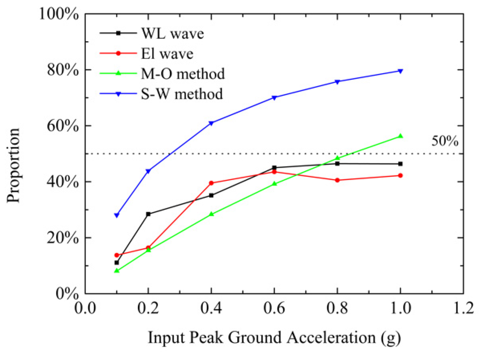
(3)
When HPGA is 1.0 g, the measured total dynamic earth force is 10.68 kN/m, which is greater than 8.57 kN/m predicted by the S-W method, but the measured Kdyn is slightly smaller than the theoretical value of the S-W method. This is because the traditional S-W and M-O methods do not consider the reinforcement effect of geogrid on sand, resulting in a gap between the predicted value and the actual value. The calculation of earth pressure of reinforced soil-retaining walls still needs to be studied.
(4)
AASHTO and NCMA guidelines check the stress distribution of geosynthetics based on the limit equilibrium theory, allowable stress, and safety factor. This method is designed for the limit working state of retaining walls, it is considered that the load and resistance are in the limit state, and it is assumed that all reinforcements can reach the same stress state, which will lead to conservative results. The measured maximum value is 0.189 kN/m, less than the predicted values of the two guidelines.

Author Contributions

Conceptualization, H.X.; writing—original draft preparation, X.C.; visualization, H.W.; data curation, S.L.; validation, X.H.; formal Analysis, S.Z. All authors have read and agreed to the published version of the manuscript.

Funding

This research was funded by the Fundamental Research Funds for the Central Universities, grant number ZY20215107; the Earthquake Technology Spark Program of China, grant number XH204402; and the National Natural Science Foundation of China, grant number 51778144.

Institutional Review Board Statement

Not applicable.

Informed Consent Statement

Not applicable.

Data Availability Statement

Not applicable.

Acknowledgments

The writers appreciate Baoshuang Jin, Guanhao Shen, Li Zhang, Shaoqiu Zhang, Jiayu Feng and Xuepeng Wang for their help in shaking table model test.

Conflicts of Interest

The authors declare no conflict of interest.

References

  1. Shi, M.; Wang, Z.; Yang, G.; Li, D. Calculation and evaluation of carbon emission from different types of retaining structures. Railw. Investig. Surv. 2020, 46, 41–48. [Google Scholar]
  2. Liu, Z. Test Study and Numerical Analysis on the Static and Dynamic Characteristics of Eco-Reinforced Earth Retaining Wall. Ph.D. Thesis, Central South University, Changsha, China, 2012. [Google Scholar]
  3. Yang, G. Study on Horizontal Deformation of Geogrid Reinforced Soil Retaining Wall. Ph.D. Thesis, Beijing Jiaotong University, Beijing, China, 2005. [Google Scholar]
  4. Wang, A. Application of Three Dimensional Drainage Flexible and Ecological Reinforced Construction in High-speed Railway Station Roadbed. In Advanced Materials Research; Trans Tech Publications Ltd.: Freienbach, Switzerland, 2012. [Google Scholar]
  5. Kazimierowicz-Frankowska, K. A case study of a geosynthetic reinforced wall with wrap-around facing. Geotext. Geomembr. 2005, 23, 107–115. [Google Scholar] [CrossRef]
  6. Wang, Z. Application of Reverse Geogrid Reinforced Soil Retaining Wall in High Retaining Wall Substation in Mountain Area. China Hyd. Elect. 2008, 6, 48–52. [Google Scholar]
  7. Koseki, J. Use of geosynthetics to improve seismic performance of earth structures. Geotext. Geomembr. 2012, 34, 51–68. [Google Scholar] [CrossRef]
  8. Krishna, A.M.; Latha, G.M. Modeling the dynamic response of wrap-faced reinforced soil retaining walls. Int. J. Geomech. 2012, 12, 439–450. [Google Scholar] [CrossRef]
  9. Murali Krishna, A.; Madhavi Latha, G. Seismic response of wrap-faced reinforced soil-retaining wall models using shaking table tests. Geosynth. Int. 2007, 14, 355–364. [Google Scholar] [CrossRef]
  10. Sakaguchi, M. A Study of the Seismic Behavior of Geosynthetic Reinforced Walls in Japan. Geosynth. Int. 1996, 3, 13–30. [Google Scholar] [CrossRef]
  11. Ramakrishnan, S.; Budhu, M.; Britto, A. Laboratory Seismic Tests of Geotextile Wrap-Faced and Geotextile- Reinforced Segmental Retaining Walls. Geosynth. Int. 1998, 5, 55–71. [Google Scholar] [CrossRef]
  12. Huang, C.C. Seismic responses of vertical-faced wrap-around reinforced soil walls. Geosynth. Int. 2019, 26, 146–163. [Google Scholar] [CrossRef]
  13. Nova-Roessig, L. Centrifuge Studies of the Seismic Response of Reinforced Soil Slopes. Ph.D. Thesis, University of California, Los Angeles, CA, USA, 1999. [Google Scholar]
  14. Nova-Roessig, L.; Sitar, N. Centrifuge Model Studies of the Seismic Response of Reinforced Soil Slopes. J. Geotech. Geoenviron. 2006, 132, 380–400. [Google Scholar] [CrossRef]
  15. Yang, K.H.; Hung, W.Y.; Kencana, E.Y. Acceleration-Amplified Responses of Geosynthetic-Reinforced Soil Structures with a Wide Range of Input Ground Accelerations. In Proceedings of the Geo-Congress, San Diego, CA, USA, 3–7 March 2013. [Google Scholar]
  16. Zhu, H.W.; Yao, L.K.; Liu, Z.S. Analysis of deformation characteristics of flexible retaining wall under earthquake. Chin. J. Rock. Mech. Eng. 2012, 31, 2829–2838. [Google Scholar]
  17. Duan, Z.C. Experimental Study on Seismic Characteristics of Encapsulated Reinforced Soil Retaining Wall. Master’s Thesis, Southwest Jiaotong University, Chengdu, China, 2011. [Google Scholar]
  18. Wang, L.M.; Xia, K.; Liu, K.; Wang, Q.; Jia, P.; Chai, S.F. A Review of Research Trends and Progress in Geotechnical Earthquake Engineering: The 16h European Conference on Earthquake Engineering. China Earthq. Eng. J. 2018, 40, 1133–1152. [Google Scholar]
  19. Li, S.H. Dynamic Response of Reinforced Soil Retaining Walls and Seismic Design Methods. Ph.D. Thesis, Institute of Engineering Mechanics, China Earthquake Administration, Harbin, China, 2021. [Google Scholar]
  20. Xue, J.; Aloisio, A.; Lin, Y.; Fragiacomo, M.; Briseghella, B. Optimum design of piles with pre-hole filled with high-damping material: Experimental tests and analytical modeling. Soil Dyn. Earthq. Eng. 2021, 151, 106995. [Google Scholar] [CrossRef]
  21. Fiorentino, G.; Cengiz, C.; De Luca, F.; Mylonakis, G.; Karamitros, D.; Dietz, M.; Nuti, C. Integral abutment bridges: Investigation of seismic soil-structure interaction effects by shaking table testing. Earthq. Eng. Struct. Dyn. 2021, 50, 1517–1538. [Google Scholar] [CrossRef]
  22. Sabermahani, M.; Ghalandarzadeh, A.; Fakher, A. Experimental study on seismic deformation modes of reinforced-soil walls. Geotext. Geomembr. 2009, 27, 121–136. [Google Scholar] [CrossRef]
  23. Eftekhari, Z.; Panah, A.K. 1-g shaking table investigation on seismic performance of polymeric-strip reinforced-soil retaining walls built on rock slopes with limited reinforced zone. Soil Dyn. Earthq. Eng. 2021, 147, 106758. [Google Scholar] [CrossRef]
  24. ASTM D6637; Standard Test Method for Determining Tensile Properties of Geogrids by the Single or Multi-rib Tensile Method. American Society of Testing Materials: West Conshohocken, PA, USA, 2015.
  25. Viswanadham, B.; Konig, D. Studies on scaling and instrumentation of a geogrid. Geotext. Geomembr. 2004, 22, 307–328. [Google Scholar] [CrossRef]
  26. El-Emam, M.M.; Bathurst, R.J. Facing contribution to seismic response of reduced-scale reinforced soil walls. Geosynth. Int. 2005, 12, 215–238. [Google Scholar] [CrossRef]
  27. Cai, X.G.; Li, S.H.; Xu, H.L.; Jing, L.P.; Huang, X.; Zhu, C. Shaking Table Study on the Seismic Performance of Geogrid Reinforced Soil Retaining Wall. Adv. Civ. Eng. 2021, 2021, 6668713.28. [Google Scholar] [CrossRef]
  28. Koseki, J.; Munaf, Y.; Tatsuoka, F.; Tateyama, M.; Kojima, K.; Sato, T. Shaking and Tilt Table Tests of Geosynthetic-Reinforced Soil and Conventional-Type Retaining Walls. Geosynth. Int. 1998, 5, 73–96. [Google Scholar] [CrossRef]
  29. Li, S.H.; Cai, X.G.; Jing, L.P.; Xu, H.L.; Huang, X.; Zhu, C. Lateral displacement control of modular-block reinforced soil retaining walls under horizontal seismic loading. Soil Dyn. Earthq. Eng. 2020, 141, 106485. [Google Scholar] [CrossRef]
  30. El-Emam, M.M.; Bathurst, R.J. Influence of reinforcement parameters on the seismic response of reduced-scale reinforced soil retaining walls. Geotext. Geomembr. 2007, 25, 33–49. [Google Scholar] [CrossRef]
  31. Yünkül, K.; Gürbüz, A. Shaking table study on seismic behavior of MSE wall with inclined backfill soils reinforced by polymeric geostrips. Geotext. Geomembr. 2022, 50, 116–136. [Google Scholar] [CrossRef]
  32. Xu, P.; Hatami, K.; Jiang, G. Shaking table study on the influence of ground motion frequency on the performance of MSE walls. Soil Dyn. Earthq. Eng. 2021, 142, 106585. [Google Scholar] [CrossRef]
  33. Athanasopoulos-Zekkos, A.; Vlachakis, V.S.; Athanasopoulos, G.A. Phasing issues in the seismic response of yielding, gravity-type earth retaining walls—Overview and results from a FEM study. Soil Dyn. Earthq. Eng. 2013, 55, 59–70. [Google Scholar] [CrossRef]
  34. Jo, S.B.; Ha, J.G.; Yoo, M.; Choo, Y.W.; Kim, D.S. Seismic behavior of an inverted T-shape flexible retaining wall via dynamic centrifuge tests. Bull. Earthq. Eng. 2014, 12, 961–980. [Google Scholar] [CrossRef]
  35. Bathurst, R.J.; Cai, Z. Pseudo-Static Seismic Analysis of Geosynthetic-Reinforced Segmental Retaining Walls. Geosynth. Int. 1995, 2, 787–830. [Google Scholar] [CrossRef]
  36. Wilson, P.; Elgamal, A. Shake table lateral earth pressure testing with dense c-phi backfill. Soil Dyn. Earthq. Eng. 2015, 71, 13–26. [Google Scholar] [CrossRef]
  37. Niu, X.D.; Yang, G.Q.; Wang, H.; Ding, S.; Feng, F. Field tests on structural properties of reinforced retaining walls with different panels. Rock Soil Mech. 2021, 42, 245–254. [Google Scholar]
  38. Jamnani, A.R.; Yazdandoust, M.; Sabermahani, M. Effect of a two-tiered configuration on the seismic behavior of reinforced soil walls. Geosynth. Int. 2022, in press. [CrossRef]
  39. Ren, F.F.; Zhang, F.; Xu, C.; Wang, G. Seismic evaluation of reinforced-soil segmental retaining walls. Geotext. Geomembr. 2016, 44, 604–614. [Google Scholar] [CrossRef]
  40. El-Emam, M.M.; Bathurst, R.J. Experimental Design, Instrumentation and Interpretation of Reinforced Soil Wall Response Using a Shaking Table. Int. J. Phys. Model. Geotech. 2004, 4, 13–32. [Google Scholar]
  41. Kilic, I.E.; Cengiz, C.; Edincliler, A.; Guler, E. Seismic behavior of geosynthetic-reinforced retaining walls backfilled with cohesive soil. Geotext. Geomembr. 2021, 49, 1256–1269. [Google Scholar] [CrossRef]
  42. Sizkow, S.F.; Shamy, U.E. Discrete-Element Method Simulations of the Seismic Response of Flexible Retaining Walls. J. Geotech. Geoenviron. 2021, 147, 04020157. [Google Scholar] [CrossRef]
  43. Liu, S.H.; Jia, F.; Chen, X.L.; Li, L.J. Experimental study on seismic response of soilbags-built retaining wall. Geotext. Geomembr. 2020, 48, 603–613. [Google Scholar] [CrossRef]
  44. NCMA TR 127B; Design Manual for Segmental Retaining Walls. National Concrete Masonry Association: Herndon, VA, USA, 2012.
  45. AASHTO LRFDUS-8; Bridge Design Specifications. American Association of State Highway and Transportation Officials: Washington, DC, USA, 2017.
Figure 1. Wrapped-face reinforced soil-retaining wall not damaged during the 2011 Tohoku earthquake, off the pacific coast [7].
Sustainability 14 09741 g001
Figure 2. Test model diagram.
Sustainability 14 09741 g002
Figure 3. Grain composition curve of the soil.
Sustainability 14 09741 g003
Figure 4. Ground motion time history curve: (a) WL wave time history curve; (b) Fourier spectrum of WL wave; (c) El wave time history curve; (d) Elwave Fourier spectrum.
Sustainability 14 09741 g004
Figure 5. Seismic damage of retaining wall model.
Sustainability 14 09741 g005
Figure 6. Acceleration amplification coefficient at different positions: (a) WL wave; (b) El wave.
Sustainability 14 09741 g006aSustainability 14 09741 g006b
Figure 7. Natural frequency and damping ratio curve.
Sustainability 14 09741 g007
Figure 8. Wall horizontal displacement distribution: (a) WL wave; (b) El wave.
Sustainability 14 09741 g008
Figure 9. Cumulative residual displacement.
Sustainability 14 09741 g009
Figure 10. Cumulative residual settlement.
Sustainability 14 09741 g010
Figure 11. The total dynamic earth force and the normalized point of application for the resultant of total dynamic earth force.
Sustainability 14 09741 g011
Figure 12. The dynamic increment active earth pressured coefficient and the normalized point of application for the resultant of the dynamic earth force increment.
Sustainability 14 09741 g012
Figure 13. The ratio of dynamic earth force increment to total dynamic earth force.
Sustainability 14 09741 g013
Figure 14. Horizontal static earth pressure: (a) WL wave; (b) El wave.
Sustainability 14 09741 g014
Figure 15. Comparison between the increment of reinforcement tensile force at the connection and the dynamic earth force increment: (a) WL wave; (b) El wave.
Sustainability 14 09741 g015
Figure 16. Increment of reinforcement tensile force at the connection: (a) WL wave; (b) El wave.
Sustainability 14 09741 g016
Figure 17. The normalized point of application for the resultant of reinforcement tension increment and dynamic earth force increment.
Sustainability 14 09741 g017
Table 2. Similitude laws in model test.
ParameterUnitScale Factor
(Prototype/Model)
Scale Factor Used in
This Study
(Prototype/Model)
LengthmN *3
Elastic moduluskPa11
DensityKg/m311
StresskPa11
TimesN0.51.73
Velocitym/sN0.51.73
Accelerationg11
Gravityg11
FrequencyHzN−0.50.58
* N: symbolized the scale of prototype to physical model (in present study its equals 3).
Table 3. Loading cases.
Case NumberInput WavePGA/gCase Code
1, 2WL, El0.1WL 0.1 g, El 0.1 g
3, 4WL, El0.2WL 0.2 g, El 0.2 g
5, 6WL, El0.4WL 0.4 g, El 0.4 g
7, 8WL, El0.6WL 0.6 g, El 0.6 g
9, 10WL, El0.8WL 0.8 g, El 0.8 g
11, 12WL, El1.0WL 1.0 g, El 1.0 g
Publisher’s Note: MDPI stays neutral with regard to jurisdictional claims in published maps and institutional affiliations.

