
Significance of Thermal Phenomena and Mechanisms of Heat Transfer through the Dynamics of Second-Grade Micropolar Nanofluids

 ,
,  , , and
Abstract
:1. Introduction
2. Mathematical Analysis
3. Solution Procedure
4. Results Validation
5. Simulated Results
5.1. Velocity Profile
5.2. Temperature Profile
5.3. Concentration Profile
5.4. Numerical Analysis
6. Conclusions
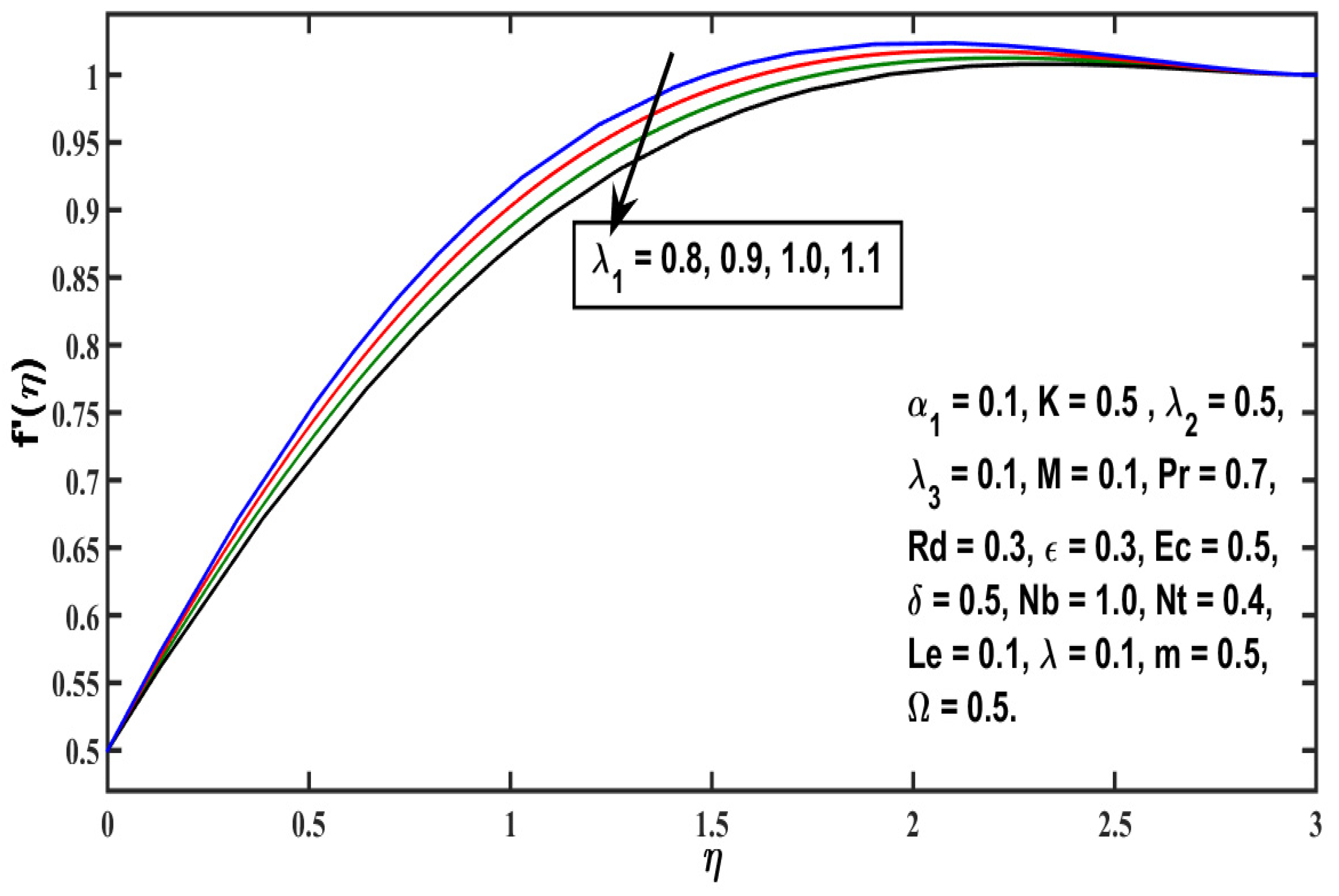
- Velocity distribution rises with higher values of any second-grade material (), local Grashof number (), modified Hartmaan number (M), or and it falls for higher values of the micropolar material parameter ( or the thermal local Grashof number (;
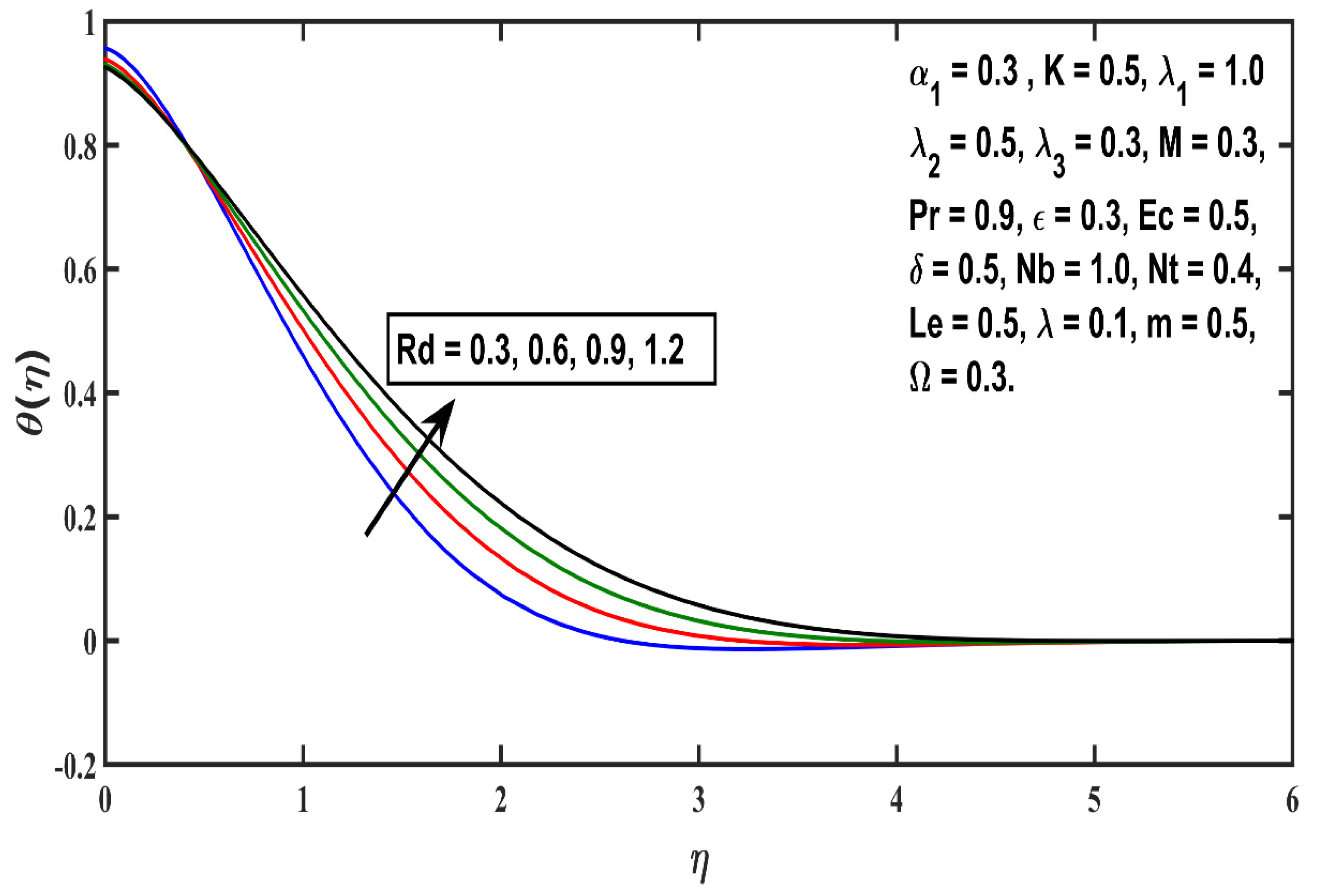
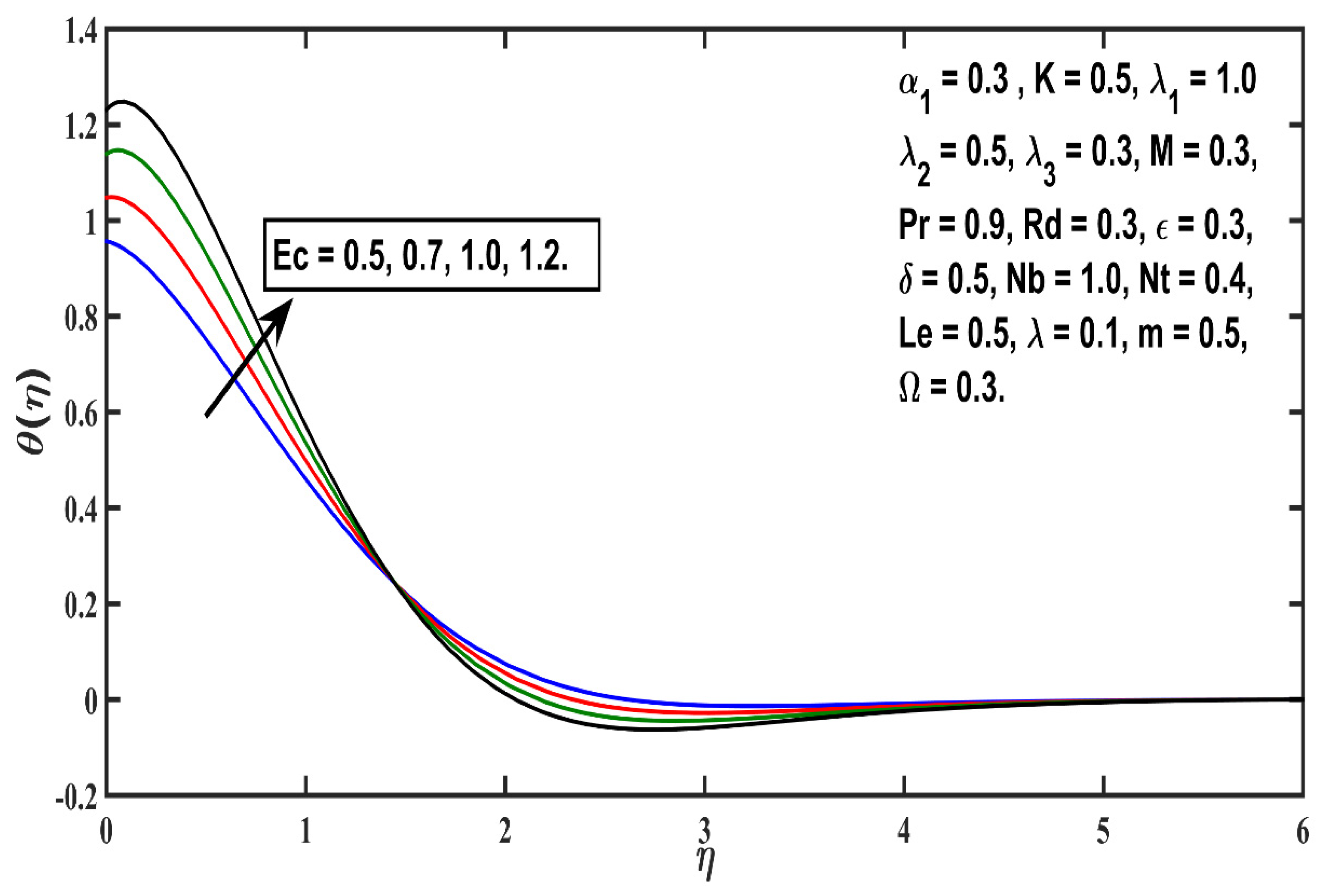
- The thickness of the thermal boundary layer boosts with thermophoretic value (Nt), Eckert number (Ec), heat source (δ), and micropolar material (K) parameters, but an opposite trend is reported against Prandtl number (Pr);
- The concentration distribution Φ(η) keeps rising against the boosting values of Brownian motion (Nb), but an inverse trend is noted against thermophoresis (Nt);
- Skin friction coefficient keeps increasing for larger values of and M, and an opposite behavior is seen for the parameters and ;
- Sherwood number increases for the increasing parameters , and and it decreases if any value of or is increased;
- keeps increasing for larger values of and M, and an opposite behavior is observed for the parameters and
Author Contributions
Funding
Institutional Review Board Statement
Informed Consent Statement
Data Availability Statement
Acknowledgments
Conflicts of Interest
Nomenclature
| Symbols | Description | Symbols | Description |
| u, v | Velocity components along and axes | Coefficient of Brownian diffusion | |
| x, y | Cartesian coordinates | Coefficient of Thermophoresis diffusion | |
| K | Thermal conductance | Heat capacitance | |
| G | Gravitational acceleration | Radiative heat flux | |
| N | Micro-rotation vector | Q | Heat source |
| J | Micro-inertia density | Free stream temperature | |
| T | Fluid’s temperature | Temperature at surface | |
| C | Concentration of fluid | Free stream velocity | |
| Free stream concentration | Greek Letters | ||
| Dimensionless velocity profile | Dimensionless variable | ||
| Dimensionless micropolar profile | Fluid’s kinematic viscosity | ||
| Dimensionless concentration profile | Fluid’s density | ||
| Dimensionless temperature distribution | Thermal diffusivity | ||
| Nb | Brownian motion parameter | Thermal expansion coefficient | |
| Le | Lewis no. | Ratio of heat capacity of nanofluid and base liquid | |
| Nt | Thermophoresis parameter | Non-dimensional stream function | |
| K | Micropolar parameter | Dynamic viscosity | |
| M | Hartmann no. | Local Grashof no. | |
| Ec | Eckert no. | Modified Grashof no. | |
| Rd | Radiation parameter | ,, | Dimensionless no. |
References
- Sakiadis, B.C. Boundary-layer behavior on continuous solid surfaces: I. Boundary-layer equations for two-dimensional and axisymmetric flow. AIChE J. 1961, 7, 26–28. [Google Scholar] [CrossRef]
- Sakiadis, B.C. Boundary-layer behavior on continuous solid surfaces: II. The boundary layer on a continuous flat surface. AIChE J. 1961, 7, 221–225. [Google Scholar] [CrossRef]
- Crane, L. Flow past a stretching plate. J. Appl. Math. Phys. 1970, 21, 645–647. [Google Scholar] [CrossRef]
- Magyari, E.; Keller, B. Heat and mass transfer in the boundary layers on an exponentially stretching continuous surface. J. Phys. D: Appl. Phys. 1999, 32, 577–585. [Google Scholar] [CrossRef]
- Elbashbeshy, E.M.A. Heat transfer over an exponentially stretching continuous surface with suction. Arch. Mech. 2001, 53, 643–651. [Google Scholar]
- Khan, S.K.; Sanjayanand, E. Viscoelastic boundary layer flow and heat transfer over an exponential stretching sheet. Int. J. Heat Mass Transf. 2005, 48, 1534–1542. [Google Scholar] [CrossRef]
- Sajid, M.; Hayat, T. Influence of thermal radiation on the boundary layer flow due to an exponentially stretching sheet. Int. Commun. Heat Mass Transf. 2008, 35, 347–356. [Google Scholar] [CrossRef]
- Ali, B.; Hussain, S.; Nie, Y.; Hussein, A.K.; Habib, D. Finite element investigation of Dufour and Soret impacts on MHD rotating flow of Oldroyd-B nanofluid over a stretching sheet with double diffusion Cattaneo Christov heat flux model. Powder Technol. 2021, 377, 439–452. [Google Scholar] [CrossRef]
- Ali, B.; Rasool, G.; Hussain, S.; Baleanu, D.; Bano, S. Finite Element Study of Magnetohydrodynamics (MHD) and Activation Energy in Darcy–Forchheimer Rotating Flow of Casson Carreau Nanofluid. Processes 2020, 8, 1185. [Google Scholar] [CrossRef]
- Ali, B.; Nie, Y.; Khan, S.A.; Sadiq, M.T.; Tariq, M. Finite Element Simulation of Multiple Slip Effects on MHD Unsteady Maxwell Nanofluid Flow over a Permeable Stretching Sheet with Radiation and Thermo-Diffusion in the Presence of Chemical Reaction. Processes 2019, 7, 628. [Google Scholar] [CrossRef] [Green Version]
- Choi, S.U.; Eastman, J.A. Enhancing Thermal Conductivity of Fluids with Nanoparticles (No. ANL/MSD/CP-84938; CONF-951135-29); Argonne National Lab: Argonne, IL, USA, 1995. [Google Scholar]
- Mabood, F.; Khan, W.A.; Ismail, A.M. MHD boundary layer flow and heat transfer of nanofluids over a non-linear stretching sheet: A numerical study. J. Magn. Magn. Mater. 2015, 374, 569–576. [Google Scholar] [CrossRef]
- Ali, B.; Nie, Y.; Hussain, S.; Habib, D.; Abdal, S. Insight into the dynamics of fluid conveying tiny particles over a rotating surface subject to Cattaneo–Christov heat transfer, Coriolis force, and Arrhenius activation energy. Comput. Math. Appl. 2021, 93, 130–143. [Google Scholar] [CrossRef]
- Bahiraei, M.; Mazaheri, N.; Hanooni, M. Employing a novel crimped-spiral rib inside a triple-tube heat exchanger working with a nanofluid for solar thermal applications: Irreversibility characteristics. Sustain. Energy Technol. Assess. 2022, 52, 102080. [Google Scholar] [CrossRef]
- Bahiraei, M.; Monavari, A. Irreversibility characteristics of a mini shell and tube heat exchanger operating with a nanofluid considering effects of fins and nanoparticle shape. Powder Technol. 2022, 398, 117117. [Google Scholar] [CrossRef]
- Mohanty, B.; Jena, S.; Pattnaik, P.K. MHD nanofluid flow over stretching/shrinking surface in presence of heat radiation using numerical method. Int. J. Emerg. Technol. 2019, 10, 119–125. [Google Scholar]
- Awan, A.U.; Abid, S.; Ullah, N.; Nadeem, S. Magnetohydrodynamic oblique stagnation point flow of second grade fluid over an oscillatory stretching surface. Results Phys. 2020, 18, 103233. [Google Scholar] [CrossRef]
- Awan, A.U.; Abid, S.; Abbas, N. Theoretical study of unsteady oblique stagnation point based Jaffrey nanofluid flow over an oscillatory stretching sheet. Adv. Mech. Eng. 2020, 12, 1–13. [Google Scholar] [CrossRef]
- Rashidi, M.; Sheremet, M.; Sadri, M.; Mishra, S.; Pattnaik, P.; Rabiei, F.; Abbasbandy, S.; Sahihi, H.; Erfani, E. Semi-Analytical Solution of Two-Dimensional Viscous Flow through Expanding/Contracting Gaps with Permeable Walls. Math. Comput. Appl. 2021, 26, 41. [Google Scholar] [CrossRef]
- Mazaheri, N.; Bahiraei, M.; Razi, S. Second law performance of a novel four-layer microchannel heat exchanger operating with nanofluid through a two-phase simulation. Powder Technol. 2022, 396, 673–688. [Google Scholar] [CrossRef]
- Bahiraei, M.; Monavari, A. Thermohydraulic performance and effectiveness of a mini shell and tube heat exchanger working with a nanofluid regarding effects of fins and nanoparticle shape. Adv. Powder Technol. 2021, 32, 4468–4480. [Google Scholar] [CrossRef]
- Eringen, A.C. Theory of micropolar fluids. J. Math. Mech. 1966, 16, 1–18. [Google Scholar] [CrossRef]
- Guram, G.; Smith, A. Stagnation flows of micropolar fluids with strong and weak interactions. Comput. Math. Appl. 1980, 6, 213–233. [Google Scholar] [CrossRef] [Green Version]
- Gorla, R.S.R.; Takhar, H.S. Boundary layer flow of micropolar fluid on rotating axisymmetric surfaces with a concentrated heat source. Acta Mech. 1994, 105, 1–10. [Google Scholar] [CrossRef]
- Gorla, R.S.R.; Mansour, M.; Mohammedien, A. Combined convection in an axisymmetric stagnation flow of micropolar fluid. Int. J. Numer. Methods Heat Fluid Flow 1996, 6, 47–55. [Google Scholar] [CrossRef]
- Nazar, R.; Amin, N. Free convection boundary layer on an isothermal sphere in a micropolar fluid. Int. Commun. Heat Mass Transf. 2002, 29, 377–386. [Google Scholar] [CrossRef]
- Nazar, R.; Amin, N.; Filip, D.; Pop, I. Stagnation point flow of a micropolar fluid towards a stretching sheet. Int. J. Non-Linear Mech. 2004, 39, 1227–1235. [Google Scholar] [CrossRef]
- Abo-Eldahab, E.M.; Ghonaim, A.F. Radiation effect on heat transfer of a micropolar fluid through a porous medium. Appl. Math. Comput. 2005, 169, 500–510. [Google Scholar] [CrossRef]
- Ishak, A. Thermal boundary layer flow over a stretching sheet in a micropolar fluid with radiation effect. Meccanica 2010, 45, 367–373. [Google Scholar] [CrossRef]
- Nadeem, S.; Hussain, M.; Naz, M. MHD stagnation flow of a micropolar fluid through a porous medium. Meccanica 2010, 45, 869–880. [Google Scholar] [CrossRef]
- Yacob, N.A.M.; Ishak, A. Micropolar fluid flow over a shrinking sheet. Meccanica 2012, 47, 293–299. [Google Scholar] [CrossRef]
- Wang, F.; Asjad, M.I.; Zahid, M.; Iqbal, A.; Ahmad, H.; Alsulami, M.D. Unsteady thermal transport flow of Casson nanofluids with generalized Mittag–Leffler kernel of Prabhakar’s type. J. Mater. Res. Technol. 2021, 14, 1292–1300. [Google Scholar] [CrossRef]
- Wang, F.; Zhang, J.; Algarni, S.; Khan, M.N.; Alqahtani, T.; Ahmad, S. Numerical simulation of hybrid Casson nanofluid flow by the influence of magnetic dipole and gyrotactic microorganism. Waves Random Complex Media 2022, 32, 1–16. [Google Scholar] [CrossRef]
- Hayat, T.; Ahmad, S.; Khan, M.I.; Alsaedi, A. Non-Darcy Forchheimer flow of ferromagnetic second grade fluid. Results Phys. 2017, 7, 3419–3424. [Google Scholar] [CrossRef]
- Ray, S.S.; Bera, R. Analytical solution of the Bagley Torvik equation by Adomian decomposition method. Appl. Math. Comput. 2005, 168, 398–410. [Google Scholar] [CrossRef]
- Meerschaert, M.M.; Tadjeran, C. Finite difference approximations for two-sided space-fractional partial differential equations. Appl. Numer. Math. 2006, 56, 80–90. [Google Scholar] [CrossRef]
- Ali, L.; Liu, X.; Ali, B.; Mujeed, S.; Abdal, S. Finite Element Analysis of Thermo-Diffusion and Multi-Slip Effects on MHD Unsteady Flow of Casson Nano-Fluid over a Shrinking/Stretching Sheet with Radiation and Heat Source. Appl. Sci. 2019, 9, 5217. [Google Scholar] [CrossRef] [Green Version]
- Zhang, X.; Zhao, J.; Liu, J.; Tang, B. Homotopy perturbation method for two dimensional time-fractional wave equation. Appl. Math. Model. 2014, 38, 5545–5552. [Google Scholar] [CrossRef]
- Prakash, A. Analytical method for space-fractional telegraph equation by homotopy perturbation transform method. Nonlinear Eng. 2016, 5. [Google Scholar] [CrossRef]
- Dhaigude, C.D.; Nikam, V.R. Solution of fractional partial differential equations using iterative method. Fract. Calc. Appl. Anal. 2012, 15, 684–699. [Google Scholar] [CrossRef]
- Abbas, N.; Malik, M.Y.; Nadeem, S.; Alarifi, I.M. On extended version of Yamada–Ota and Xue models of hybrid nanofluid on moving needle. Eur. Phys. J. Plus 2020, 135, 145. [Google Scholar] [CrossRef]
- Khan, U.; Shafiq, A.; Zaib, A.; Sherif, E.-S.M.; Baleanu, D. MHD Radiative Blood Flow Embracing Gold Particles via a Slippery Sheet through an Erratic Heat Sink/Source. Mathematics 2020, 8, 1597. [Google Scholar] [CrossRef]
- Irfan, M.; Khan, W.A.; Khan, M.; Waqas, M. Evaluation of Arrhenius activation energy and new mass flux condition in Carreau nanofluid: Dual solutions. Appl. Nanosci. 2020, 10, 5279–5289. [Google Scholar] [CrossRef]
- Ramzan, M.; Riasat, S.; Kadry, S.; Chu, Y.-M.; Ghazwani, H.A.S.; Alzahrani, A.K. Influence of autocatalytic chemical reaction with heterogeneous catalysis in the flow of Ostwald-de-Waele nanofluid past a rotating disk with variable thickness in porous media. Int. Commun. Heat Mass Transf. 2021, 128, 105653. [Google Scholar] [CrossRef]
- Ali, B.; Yu, X.; Sadiq, M.T.; Rehman, A.U.; Ali, L. A Finite Element Simulation of the Active and Passive Controls of the MHD Effect on an Axisymmetric Nanofluid Flow with Thermo-Diffusion over a Radially Stretched Sheet. Processes 2020, 8, 207. [Google Scholar] [CrossRef] [Green Version]


| Skin Friction Coefficient (RK 4th Order) | Skin Friction Coefficient (Bvp4c) | |||
|---|---|---|---|---|
| (m = 0.5) | (m = 0.0) | (m = 0.5) | (m = 0.0) | |
| 0.5 | 1.1948 | 0.9913 | 1.19476 | 0.99127 |
| 0.6 | 1.1423 | 0.9257 | 1.14227 | 0.92568 |
| 0.7 | 1.0948 | 0.8692 | 1.09476 | 0.86915 |
| 0.8 | 1.0518 | 0.8200 | 1.05175 | 0.81996 |
| Nusselt Number (RK 4th Order) | Nusselt Number (Bvp4c) | |||
| (m = 0.5) | (m = 0.0) | (m = 0.5) | (m = 0.0) | |
| 0.5 | 0.3434 | 0.3524 | 0.34336 | 0.35235 |
| 0.6 | 0.3829 | 0.3918 | 0.38285 | 0.39177 |
| 0.7 | 0.4222 | 0.4304 | 0.42217 | 0.43036 |
| 0.8 | 0.4611 | 0.4685 | 0.46108 | 0.46847 |
| Skin Friction Coefficient | ||||||||
|---|---|---|---|---|---|---|---|---|
| (m = 0.5) | (m = 0) | |||||||
| 0.5 | 0.5 | 0.5 | 0.5 | 0.5 | 0.4 | 0.5 | 1.1948 | 0.9913 |
| 0.6 | 1.1423 | 0.9257 | ||||||
| 0.7 | 1.0948 | 0.8692 | ||||||
| 0.8 | 1.0518 | 0.8200 | ||||||
| 0.5 | 0.3 | 1.0070 | 0.8592 | |||||
| 0.4 | 1.0980 | 0.9236 | ||||||
| 0.5 | 1.1948 | 0.9913 | ||||||
| 0.6 | 1.2928 | 1.0598 | ||||||
| 0.5 | 0.5 | 1.1948 | 0.9913 | |||||
| 0.7 | 1.1184 | 0.9264 | ||||||
| 0.9 | 1.0394 | 0.8596 | ||||||
| 1.1 | 0.9577 | 0.7905 | ||||||
| 0.5 | 0.4 | 1.0701 | 0.8893 | |||||
| 0.45 | 1.1325 | 0.9404 | ||||||
| 0.50 | 1.1948 | 0.9913 | ||||||
| 0.55 | 1.2569 | 1.0420 | ||||||
| 0.5 | 0.1 | 1.4001 | 1.1549 | |||||
| 0.3 | 1.2827 | 1.0615 | ||||||
| 0.5 | 1.1948 | 0.9913 | ||||||
| 0.7 | 1.1278 | 0.9377 | ||||||
| 0.5 | 0.0 | 0.7635 | 0.6420 | |||||
| 0.2 | 0.9747 | 0.9913 | ||||||
| 0.4 | 1.1948 | 0.9924 | ||||||
| 0.6 | 1.4235 | 1.1732 | ||||||
| 0.4 | 0.2 | 1.4670 | 1.2111 | |||||
| 0.3 | 1.3787 | 1.1403 | ||||||
| 0.4 | 1.2879 | 1.0670 | ||||||
| 0.5 | 1.1948 | 0.9913 | ||||||
| Nusselt Number | |||||||||||
|---|---|---|---|---|---|---|---|---|---|---|---|
| (m = 0.5) | (m = 0) | ||||||||||
| 0.5 | 0.9 | 0.3 | 0.3 | 0.5 | 0.5 | 1.2 | 0.7 | 0.5 | 0.5 | 0.3434 | 0.3524 |
| 0.6 | 0.3829 | 0.3918 | |||||||||
| 0.7 | 0.4222 | 0.4304 | |||||||||
| 0.8 | 0.4611 | 0.4685 | |||||||||
| 0.5 | 0.7 | 0.1784 | 0.1810 | ||||||||
| 0.9 | 0.3434 | 0.3524 | |||||||||
| 1.4 | 0.7401 | 0.7754 | |||||||||
| 2.1 | 1.2515 | 1.3415 | |||||||||
| 0.9 | 0.3 | 0.3434 | 0.3524 | ||||||||
| 0.5 | 0.3422 | 0.3502 | |||||||||
| 0.6 | 0.3386 | 0.3460 | |||||||||
| 0.7 | 0.3332 | 0.3400 | |||||||||
| 0.3 | 0.2 | 0.3591 | 0.3692 | ||||||||
| 0.25 | 0.3511 | 0.3606 | |||||||||
| 0.3 | 0.3434 | 0.3524 | |||||||||
| 0.35 | 0.3359 | 0.3444 | |||||||||
| 0.3 | 0.5 | 0.3434 | 0.3524 | ||||||||
| 0.55 | 0.3991 | 0.4069 | |||||||||
| 0.6 | 0.4550 | 0.4616 | |||||||||
| 0.65 | 0.5110 | 0.5164 | |||||||||
| 0.5 | 0.4 | 0.2117 | 0.2149 | ||||||||
| 0.45 | 0.2750 | 0.2809 | |||||||||
| 0.5 | 0.3434 | 0.3524 | |||||||||
| 0.55 | 0.4174 | 0.4300 | |||||||||
| 0.5 | 1.0 | 0.3453 | 0.3541 | ||||||||
| 1.1 | 0.3442 | 0.3532 | |||||||||
| 1.2 | 0.3434 | 0.3524 | |||||||||
| 1.3 | 0.3426 | 0.3517 | |||||||||
| 1.2 | 0.7 | 0.3434 | 0.3524 | ||||||||
| 0.8 | 0.3509 | 0.3596 | |||||||||
| 0.9 | 0.3585 | 0.3669 | |||||||||
| 1.0 | 0.3661 | 0.3741 | |||||||||
| 0.7 | 0.3 | 0.3538 | 0.3621 | ||||||||
| 0.5 | 0.3434 | 0.3524 | |||||||||
| 0.6 | 0.3384 | 0.3478 | |||||||||
| 0.7 | 0.3336 | 0.3432 | |||||||||
| 0.5 | 0.4 | 0.3373 | 0.3463 | ||||||||
| 0.5 | 0.3434 | 0.3524 | |||||||||
| 0.6 | 0.3490 | 0.3581 | |||||||||
| 0.7 | 0.3544 | 0.3635 | |||||||||
| Sherwood Number | |||||||||||
|---|---|---|---|---|---|---|---|---|---|---|---|
| (m = 0.5) | (m = 0) | ||||||||||
| 0.5 | 0.9 | 0.3 | 0.3 | 0.5 | 0.5 | 1.2 | 0.7 | 0.5 | 0.5 | 0.1170 | 0.1201 |
| 0.6 | 0.1303 | 0.1332 | |||||||||
| 0.7 | 0.1433 | 0.1461 | |||||||||
| 0.8 | 0.1562 | 0.1587 | |||||||||
| 0.5 | 0.7 | 0.0613 | 0.0622 | ||||||||
| 0.9 | 0.1170 | 0.1201 | |||||||||
| 1.4 | 0.2474 | 0.2588 | |||||||||
| 2.1 | 0.4086 | 0.4363 | |||||||||
| 0.9 | 0.3 | 0.1170 | 0.1201 | ||||||||
| 0.5 | 0.1011 | 0.1035 | |||||||||
| 0.6 | 0.0938 | 0.0958 | |||||||||
| 0.7 | 0.0869 | 0.0886 | |||||||||
| 0.3 | 0.2 | 0.1301 | 0.1337 | ||||||||
| 0.25 | 0.1233 | 0.1266 | |||||||||
| 0.3 | 0.1170 | 0.1201 | |||||||||
| 0.35 | 0.1112 | 0.1140 | |||||||||
| 0.3 | 0.5 | 0.1170 | 0.1201 | ||||||||
| 0.55 | 0.1356 | 0.1382 | |||||||||
| 0.6 | 0.1542 | 0.1564 | |||||||||
| 0.65 | 0.1727 | 0.1745 | |||||||||
| 0.5 | 0.4 | 0.0726 | 0.0737 | ||||||||
| 0.45 | 0.0941 | 0.0960 | |||||||||
| 0.5 | 0.1170 | 0.1201 | |||||||||
| 0.55 | 0.1417 | 0.1459 | |||||||||
| 0.5 | 1.0 | 0.1412 | 0.1448 | ||||||||
| 1.1 | 0.1280 | 0.1313 | |||||||||
| 1.2 | 0.1170 | 0.1201 | |||||||||
| 1.3 | 0.1078 | 0.1106 | |||||||||
| 1.2 | 0.7 | 0.1170 | 0.1201 | ||||||||
| 0.8 | 0.1366 | 0.1400 | |||||||||
| 0.9 | 0.1570 | 0.1606 | |||||||||
| 1.0 | 0.1781 | 0.1819 | |||||||||
| 0.7 | 0.3 | 0.1214 | 0.1242 | ||||||||
| 0.5 | 0.1170 | 0.1201 | |||||||||
| 0.6 | 0.1150 | 0.1181 | |||||||||
| 0.7 | 0.1130 | 0.1162 | |||||||||
| 0.5 | 0.4 | 0.1150 | 0.1180 | ||||||||
| 0.5 | 0.1170 | 0.1201 | |||||||||
| 0.6 | 0.1189 | 0.1220 | |||||||||
| 0.7 | 0.1207 | 0.1238 | |||||||||
| (m = 0.5) | (m = 0) | |||||||
| 0.5 | 0.5 | 0.5 | 0.5 | 0.5 | 0.4 | 0.2 | 1.2953 | −0.8505 |
| 0.6 | 1.1323 | −0.8278 | ||||||
| 0.7 | 1.0053 | −0.8066 | ||||||
| 0.8 | 0.9034 | −0.7868 | ||||||
| 0.5 | 0.3 | 0.9691 | −0.8197 | |||||
| 0.4 | 1.1228 | −0.8359 | ||||||
| 0.5 | 1.2953 | −0.8505 | ||||||
| 0.6 | 1.4808 | −0.8632 | ||||||
| 0.5 | 0.5 | 1.2953 | −0.8505 | |||||
| 0.7 | 1.1682 | −0.8239 | ||||||
| 0.9 | 1.0363 | −0.7947 | ||||||
| 1.1 | 0.8990 | −0.7624 | ||||||
| 0.5 | 0.4 | 1.1123 | −0.8103 | |||||
| 0.45 | 1.2037 | −0.8308 | ||||||
| 0.50 | 1.2953 | −0.8505 | ||||||
| 0.55 | 1.3868 | −0.8697 | ||||||
| 0.5 | 0.1 | 1.5504 | −0.9253 | |||||
| 0.3 | 1.4042 | −0.8825 | ||||||
| 0.5 | 1.2953 | −0.8505 | ||||||
| 0.7 | 1.2126 | −0.8264 | ||||||
| 0.5 | 0.0 | 0.7539 | −0.7302 | |||||
| 0.2 | 1.0172 | −0.7915 | ||||||
| 0.4 | 1.2953 | −0.8505 | ||||||
| 0.6 | 1.5877 | −0.9075 | ||||||
| 0.4 | 0.2 | 1.2953 | −0.8505 | |||||
| 0.3 | 1.2382 | −0.7683 | ||||||
| 0.4 | 1.1805 | −0.6844 | ||||||
| 0.5 | 1.1223 | −0.5989 | ||||||
Publisher’s Note: MDPI stays neutral with regard to jurisdictional claims in published maps and institutional affiliations. |
© 2022 by the authors. Licensee MDPI, Basel, Switzerland. This article is an open access article distributed under the terms and conditions of the Creative Commons Attribution (CC BY) license (https://creativecommons.org/licenses/by/4.0/).
Share and Cite
Awan, A.U.; Ahammad, N.A.; Ali, B.; Tag-ElDin, E.M.; Guedri, K.; Gamaoun, F. Significance of Thermal Phenomena and Mechanisms of Heat Transfer through the Dynamics of Second-Grade Micropolar Nanofluids. Sustainability 2022, 14, 9361. https://doi.org/10.3390/su14159361
Awan AU, Ahammad NA, Ali B, Tag-ElDin EM, Guedri K, Gamaoun F. Significance of Thermal Phenomena and Mechanisms of Heat Transfer through the Dynamics of Second-Grade Micropolar Nanofluids. Sustainability. 2022; 14(15):9361. https://doi.org/10.3390/su14159361
Chicago/Turabian StyleAwan, Aziz Ullah, N. Ameer Ahammad, Bagh Ali, ElSayed M. Tag-ElDin, Kamel Guedri, and Fehmi Gamaoun. 2022. "Significance of Thermal Phenomena and Mechanisms of Heat Transfer through the Dynamics of Second-Grade Micropolar Nanofluids" Sustainability 14, no. 15: 9361. https://doi.org/10.3390/su14159361