Article

Rainfall Variability and Tidal Inundation Influences on Mangrove Greenness in Karimunjawa National Park, Indonesia

1
School of Environment and Society, Tokyo Institute of Technology, Ookayama, Tokyo 152-8552, Japan
2
National Research and Innovation Agency, Jakarta 10340, Indonesia
3
Department of Oceanography, Faculty of Fisheries and Marine Science, Universitas Diponegoro, Semarang 50275, Indonesia
4
Marine Research Center, Ministry of Marine Affairs and Fisheries, Jalan Pasir Putih II, Ancol Timur, Jakarta 14430, Indonesia
*
Author to whom correspondence should be addressed.
Sustainability 2022, 14(14), 8948; https://doi.org/10.3390/su14148948
Submission received: 3 June 2022 / Revised: 11 July 2022 / Accepted: 13 July 2022 / Published: 21 July 2022

Abstract

:
Mangroves, which are vulnerable to natural threats and human activities on small islands in the tropics, play an essential role as carbon sinks, helping to mitigate climate change. In this study, we discussed the effect of natural factors on mangrove sustainability by analyzing the impact of rainfall, land surface temperature (LST), and tidal inundation on the greenness of mangroves in Karimunjawa National Park (KNP), Indonesia. We used Sentinel-2 image data to obtain the normalized difference vegetation index (NDVI) and normalized difference moisture index (NDMI) during the dry season to determine the effect of inundation on mangrove greenness and soil moisture. The tidal inundation area was calculated using topographic data from the KNP and tidal observations from the area adjacent to it. Unmanned autonomous vehicles and topographic data were used to estimate mangrove canopy height. We also calculated mangrove greenness phenology and compared it to rainfall from satellite data from 2019–2021. Results show that the intertidal area is dominated by taller mangroves and has higher NDVI and NDMI values than non-intertidal areas. We also observed that mangroves in intertidal areas are mostly evergreen, and optimum greenness in KNP occurs from February to October, with maximum greenness in July. Cross-correlation analysis suggests that high rainfall affects NDVI, with peak greenness occurring three months after high rainfall. The LST and NDVI cross-correlation showed no time lag. This suggests that LST was not the main factor controlling mangrove greenness, suggesting tides and rainfall influence mangrove greenness. The mangroves are also vulnerable to climate variability and change, which limits rainfall. However, sea-level rise due to climate change might positively impact mangrove greenness.

1. Introduction

Mangroves are salt-tolerant trees and shrubs that can adapt to brackish water. Therefore, they can grow in an intertidal zone with a saline, wet environment. Mangroves grow in tropical and subtropical areas, benefiting the surrounding environment and community. One of these benefits is as a carbon dioxide (CO2) sink that helps mitigate climate change [1,2] as the ability of mangroves to absorb CO2 is up to four times greater than that of tropical terrestrial forests [3,4].
In contrast, tropical waters, including the ocean in Indonesia, are generally a CO2 source [5,6]. Therefore, the role of mangroves as carbon sinks in the tropics is crucial. Coastlines and small islands in Indonesia are potential areas for mangroves to grow and absorb carbon from the atmosphere because Indonesia has a long coastline and many small islands that have global significance in climate change mitigation [7,8]. The Java Sea in Indonesia, located north of Java Island, is where the largest population and greatest anthropogenic activities occur. A study by Wirasatriya [9] shows that the Java Sea acts as a carbon source and emits maximum CO2 during April and May. Thus, mangroves around the Java Sea play an essential role in CO2 sequestration. One area with mangroves in the Java Sea is Karimunjawa Island. Moreover, the sea around Karimunjawa Island also acts as a carbon source [10]. Therefore, the presence of mangroves on the island is very important.
However, the mangroves on the island are threatened with deterioration due to human activities and natural forces [11]. Mangrove clearing for aquaculture, ponds, and tourism facilities is a significant threat [12,13]. On the other hand, natural factors such as climate change also cause mangrove damage to small islands [14]. Furthermore, mangroves require freshwater for growth, although they can grow in brackish areas [15]. Therefore, the hydrological alteration can kill mangroves [16]. Karimunjawa Island does not have a large river that supplies freshwater to the mangroves, as on the big island. Thus, the source of freshwater for mangroves on the island comes from rainwater and groundwater [17] which vary depending on the climate. Furthermore, a study by Prihantono et al. [18] suggested that tidal inundation also affects mangrove health in KNP, in addition to groundwater and rainfall. However, the effects of rain and tidal inundation on the mangroves were not discussed in detail.
Mangrove health is related to the greenness of mangroves forests because greenness represents the canopy cover of the mangroves [11,19]. Healthy mangroves have dense green canopy cover. Canopy cover is correlated with tree height [20]. Thus, high mangroves have a wide canopy cover. Mangrove greenness is also related to the water stress surrounding it. Mangrove that grows in wet soil is healthier than in dry soil [18]. This soil moisture may come from rainfall, river flood, and tidal inundation. We can detect the greenness of mangrove forests by using the remote sensing method.
Monitoring and time-series analysis of mangrove forests using remote sensing methods have been widely used more recently and are easier to use than field surveys [21,22]. One method to monitor the health of mangrove forests as a response to climate and environmental changes in a time series is vegetation greenness phenology, or land surface phenology. This method can be performed using free satellite data with moderate resolutions [16,23,24,25,26]. Vegetation greenness phenology depicts the annual timing cycle of vegetation growth, such as leaf emergence, greenness, and senescence, driven by environmental and climate dynamics [25,27]. By knowing the green cycle of mangroves, we can determine when mangroves optimally absorb carbon in the atmosphere because of the impact of canopy capacity on photosynthesis [28,29].
For this study, we selected Karimunjawa National Park (KNP) as the study area because this area is a protected area, so the impact of human activities on mangroves is negligible. Thus, we could analyze the natural impacts on mangroves. This study aimed to examine the effects of rainfall, tidal inundation, and land surface temperature (LST) on the health or greenness of mangroves in the KNP as a representation of natural threats to mangroves on small islands, using remote sensing methods. Specifically, the objectives of this study were to (1) compare mangrove greenness, canopy height, and soil moisture in intertidal and non-intertidal areas; (2) determine the phenology metrics of mangrove greenness in the KNP by estimating the start of season (SOS), peak of season (POS), end of season (EOS), amplitude of season (AOS), and length of season (LOS); (3) estimate the greenness of mangroves due to variability in rainfall and LST; and (4) analyze why rainfall, tidal inundation, and LST can affect the greenness of mangroves.

2. Materials and Methods
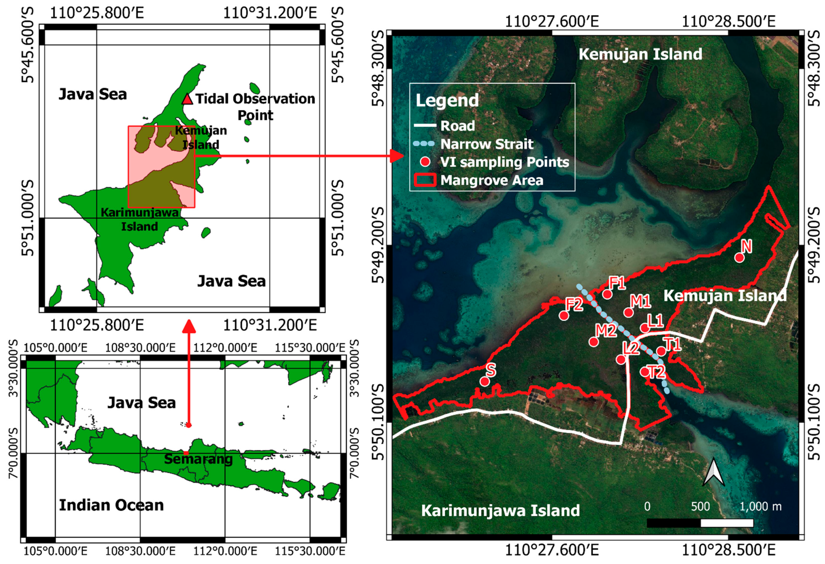
2.1. Study Site

Our study site was the KNP (Figure 1, 5°50.386′ S–5°48.844′ S, 110°26.771′ E–110°28.925′ E) in Central Java Province, Indonesia with a total area of 221.9 ha. It is located in the Java Sea and is approximately 125 km north of Semarang, the capital city of Central Java. The KNP is located on Karimunjawa and Kemujan Islands, separated by a narrow strait. This area has a humid tropical maritime climate, with average daily temperatures ranging from 26–30 °C, average humidity of 70–85%, and average annual rainfall of 2632 mm. The average monthly rainfall during the dry season (April to September) is 60 mm, and during the wet season (October to March) it is 400 mm [11].
The mangrove forest in KNP is protected by the Ministry of Environment and Forestry of Indonesia and serves as a mangrove conservation area, for tourism, education, and research [30]. This natural mangrove forest has at least 45 mangrove species growing on the coastal fringe, with Rhizophora sp. being the dominant species [11,30].
According to Karimunjawa National Park Office (BTNKJ) the Ministry of Environment and Forestry of Indonesia [31,32,33], there are three mangrove zones in KNP extending from inland to the shoreline area. The first zone is a low multi-stem stand on the landward side (points L1 and L2 in Figure 1). The dominant mangrove species in this zone are Ceriops tagal and Lumnitzera racemosa. The second zone is in the middle of the KNP (points M1 and M2 in Figure 1) and is dominated by a mangrove structure with a single and multi-stem low-closed forest. In this zone, Ceriops tagal, Lumnitzera sp., Rhizophora sp., and Bruguiera gymnorhiza, with highly mixed formations, were dominant. The third zone is in the shoreline area (points F1 and F2 in Figure 1) and is dominated by Rhizophora mucronata, some individual Bruguiera gymnorhiza, and Xylocarpus granatum with a multi-stem closed forest. In addition, the southern part of the strait along the coastline (point S, Figure 1) is dominated by tall Rhizophora sp. with a diameter of more than 10 cm. Furthermore, the eastern area of the road (points T1 and T2 in Figure 1) is dominated by tall mangroves with Scyphiphora hydrophyllacea and Rhizophora apiculate species. Meanwhile, the northern area of the strait (point N in Figure 1) is dominated by tall mangroves with Lumnitzera sp., followed by Ceriops tagal, Excoecaria agallocha, and Rhizophora apiculata. In this zone, short mangrove zones are dominated by Ceriops tagal.

2.2. Rainfall Data, Land Surface Temperature Data, and Vegetation Indices Calculation

We used monthly rainfall data from Global Precipitation Measurement (GPM) V6 satellite because it has a high correlation coefficient and small error compared to the closest meteorological station to KNP in Semarang City [18]. The GPM is an international satellite mission by the National Aeronautics and Space Administration (NASA) that provides precipitation data with a 0.1° spatial resolution, with 30 min and monthly temporal resolution. The GPM used the Integrated Multi-Satellite Retrievals for GPM (IMERG) algorithm to obtain precipitation data. This algorithm provides rainfall estimates by combining data from all passive microwave instruments in the GPM constellation with precipitation gauge analysis [34].
We used Moderate Resolution Imaging Spectroradiometer (MODIS) data (MOD11A2 V6) to obtain LST data. This data is an 8-day average of the daily MOD11A1 LST dataset with a spatial resolution of 1000 m. The 8-day compositing period was chosen because the exact ground track repeat period of the Terra and Aqua platforms is twice this period. This product includes both day and nighttime surface temperature bands and their quality indicator (QC) layers [35].
We used Sentinel-2 L2A to estimate the normalized difference vegetation index (NDVI) and normalized difference moisture index (NDMI) in this study. Sentinel-2 is an optical satellite operated by the European Space Agency (ESA) with a high spatial resolution (10–60 m) and 13 bands. Sentinel 2 can provide images over a 2–5 days timeframe at the same location. Sentinel-2 L2A indicates that this satellite image is in the form of an orthoimage Bottom-Of-Atmosphere (BOA)-corrected reflectance product. Sentinel-2 L2A in the KNP area is available in the Google Earth Engine (GEE) dataset from 15 December 2018, to the present. Thus, we did not need to manually perform the correction process to obtain the BOA reflectance image. We extracted NDVI and NDMI at the sampling point (Figure 1), in which each point has an area of 100 m2. We calculated the NDVI and NDMI from 1 January 2019, to 31 December 2021, based on the availability of the Sentinel-2 L2A dataset in GEE. Due to the monthly GPM V6 rainfall data being available until September 2021, we analyzed the NDVI and LST data from 1 January 2019, to 30 September 2021.
We applied the cloud mask algorithm to Sentinel-2 images to obtain images free from cloud cover in the KNP area. The cloud-masking algorithm in the Sentinel-2 image uses a QA60 bitmask band with a resolution of 60 m, which contains cloud information. This resolution is quite large, and sometimes clouds with a coverage of fewer than 60 m cannot be detected by this algorithm. Consequently, we could not mask the low cloud coverage in the KNP area. Therefore, we reexamined the images manually and selected clear images from the sampling point after applying the cloud mask algorithm. We used cloudy images in the KNP area if the sampling point was not covered. This was done to obtain as much free cloud time-series data of vegetation indices as possible. As a result, 149 datasets (Table S1) were obtained for calculating the NDVI. The images in January, February, and December are difficult to obtain because the cloud coverage in these months is higher than in the other months. In contrast, clear images are easily obtained in July and August because the cloud coverage is low.
The NDVI and NDMI were determined using Equations (1) and (2). The NDVI is a vegetation index used to estimate mangrove greenness associated with green and healthy vegetation because the NDVI is sensitive to chlorophyll absorbing red light and reflects the near-infrared (NIR) wavelengths due to scattering by the internal leaf structure [36,37]. NDVI values range from −1 to 1; when the value is greater than 0.3, it indicates healthy vegetation. In contrast, NDVI lower than 0.3 represent barren or drought-tolerant vegetation. The NDMI is a vegetation index for estimating the moisture of vegetation [38,39]. The equation for the NDMI is similar to the equation of the normalized difference water index (NDWI) by Gao [40]. The NDMI is sensitive to soil and plant moisture, shadowing, leaf water content, and other possible effects not yet discovered or that reflect a combination of structure and water content [38]. In this study, we used the NDMI as the soil moisture proxy, assuming that the water content in vegetation is proportional to soil wetness [18]. NDMI ranges from −1 to 1; when the value is greater than 0.4, it indicates a high canopy cover of vegetation and no water stress. In contrast, less than 0.4 represent bare soil or mid-low canopy cover of vegetation with high-low water stress. NDVI and NDMI can be used to estimate drought index to monitor drought in an area using the remote sensing method which is easier to calculate spatial distribution and resolution compared to traditionally based drought monitoring [41].
NDVI = (NIR − RED)/(NIR + RED)
NDMI = (NIR − SWIR)/(NIR + SWIR)
RED, NIR, and SWIR are the red, near-infrared, and short-wave infrared bands of the satellite image, respectively. We calculated the NDVI and NDMI by applying Equations (1) and (2) to Sentinel-2 L2A satellite imagery using the GEE. In the Sentinel-2 the RED band is band number four (B04) with a central wavelength of 665 nm, NIR is band number eight (B08) with a central wavelength of 842 nm, and SWIR is band number 11 (B11) with a central wavelength of 1610 nm.

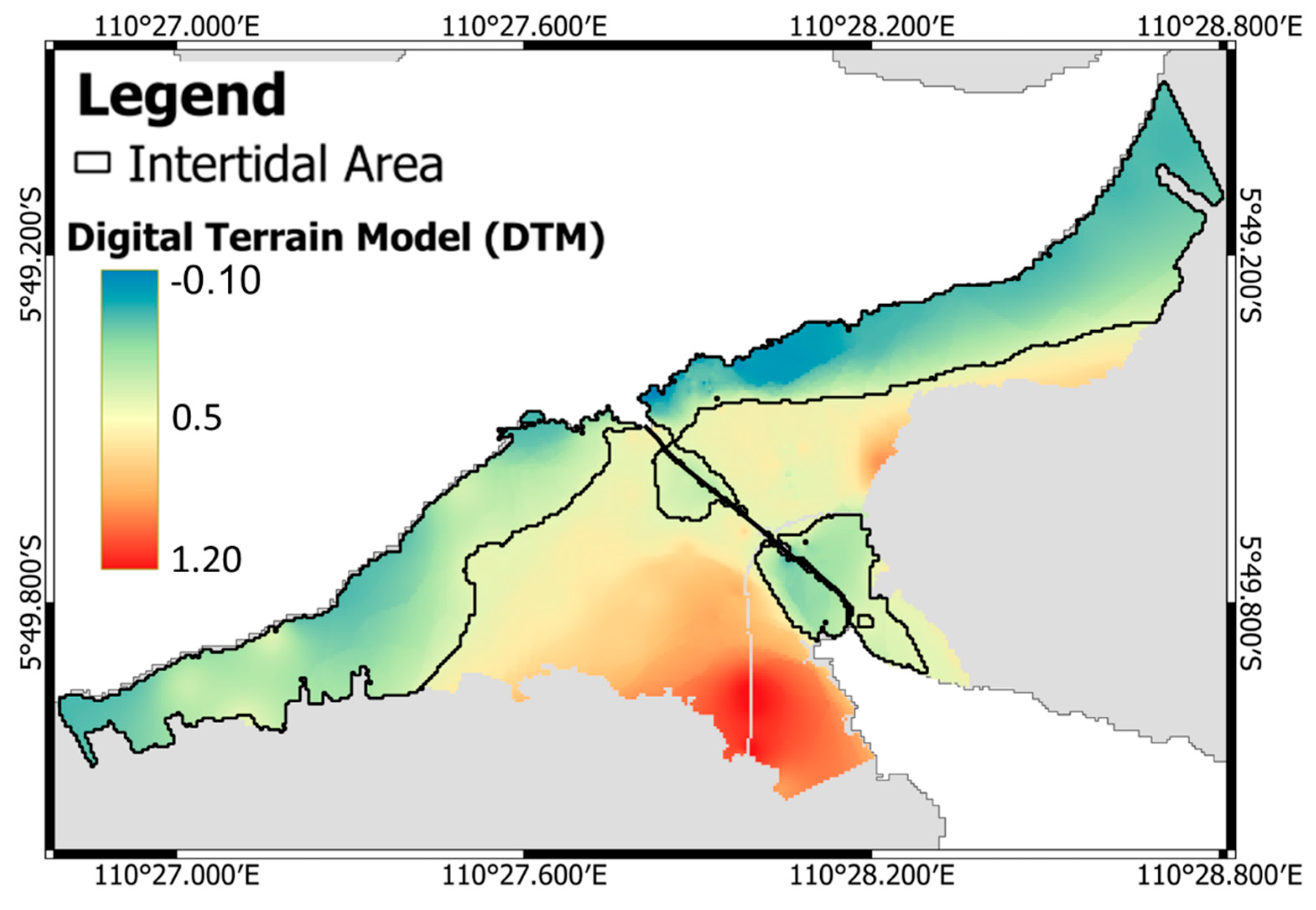
2.3. Digital Terrain Model and Mangrove Canopy Height Calculation

We used a digital terrain model (DTM) and mangrove canopy height data from the work of Wirasatriya et al. [33]. The data processing to obtain it was described in detail in their article. In summary, the DTM data were obtained by conducting a topographical survey of the mangrove area. A topographic survey was conducted using two GNSS Comnav T300 receiver units. One of the GNSS receiver units is operated using the static method as a ground control point (GCP). The other unit is operated for topographic surveys using the real-time kinematic (RTK) method. Furthermore, 7 GCPs and 60 RTK spots were obtained and were spatially distributed throughout the study area. In addition, a topographic survey using the water pass method was conducted, and 227 spots were obtained in the study area. An RTK point interpolation generates DTM data, which is then validated using water pass survey data. The results show a Root Mean Square (RMSE) of 0.08 m, which means that the DTM data show high accuracy.
Mangrove canopy height data were obtained by aerial mapping using an unmanned aerial vehicle (UAV). In simple terms, aerial mapping produces digital surface model (DSM) data, which explains the elevation of the Earth’s surface from the mean sea level. This is different from the DTM, which shows ground surface elevation from the mean sea level. Thus, mangrove canopy height data can be calculated by subtracting the DSM and DTM. The spatial resolution of this data is 15 m.

2.4. Intertidal Area Estimation

The intertidal area was estimated from tidal and topographic data in the KNP. In this study, we used tidal observation data from the Indonesia Information and Geospatial Agency (https://srgi.big.go.id/tides, accessed on 16 March 2022). The location of this tidal station is approximately 4.5 km north of the strait between Karimunjawa Island and Kemujan Island in KNP (Figure 1, 5°47.280′ S, 110°28.636′ E). We analyzed the tidal elevation from 1 October 2019, to 30 September 2021. We then calculated the mean higher high water (MHHW) in KNP using Equation (3) [42]. We used this MHHW value as the highest elevation in the intertidal area, which is frequently submerged by seawater.
MHHW = Z0 + (M2 + K1 + O1)
where Z0 is the mean sea level (MSL); in this case, the MSL is zero. M2, K1, and O1 are the amplitudes of the tidal harmonic components at 12.4, 23.9, and 25.8 h periods, respectively. The tidal harmonic components were obtained using the least-square method with the t_tide software [43].
Thus, we can determine the intertidal area by selecting a DTM elevation data pixel that is less than or equal to MHHW. However, not all these pixels are intertidal regions. Only pixels connected to the coast are defined as intertidal regions. Otherwise, the pixel is not an intertidal area, even if the value is less than the MHHW. We selected the DTM data pixels using the raster calculation tool in QGIS software version 3.16.15-Hannover, a free and open-source geographic information system (GIS) software. The output obtained was then converted into an intertidal polygon using the Polygonize (Raster to Vector) tool in QGIS software.

2.5. Pixel Extraction in the Intertidal and Non-Intertidal Area

Pixel extraction was used to determine and compare the values of NDVI, NDMI, and mangrove canopy height in the intertidal and non-intertidal areas. We used Clip Raster with the mask layer tool and then raster pixel-to-point in QGIS software to extract the pixels. This extraction step was performed after obtaining polygons of the intertidal area in the previous step, and these were used as the mask layer. We applied this step only to dry season images to determine the impact of tidal inundation without the rainfall effect. We converted the pixel count to an area by multiplying the pixel count with a pixel area of Sentinel-2 (100 m2) and a pixel area of mangrove canopy height image (225 m2) for both inundation and non-inundation areas.

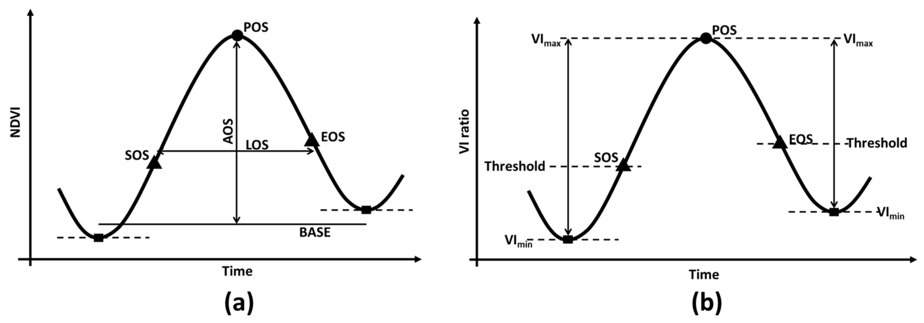
2.6. Phenology Metrics Calculation

The NDVI time series data extracted from the Sentinel-2 images shows peak and trough patterns, although this pattern is not smooth, and a large amount of scattered data makes it difficult to determine the phenology metrics. Time-series data is refined using smoothing methods, such as changing weight, Savitzky-Golay, asymmetric Gaussian, double-logistic, Whittaker Smoother, and harmonic regression [44,45]. In this study, we use the harmonic regression method because of its advantages in terms of simplicity, low computational cost, and accuracy for filling gaps in time-series data [46,47,48]. The popular harmonic regression method used for determining phenological metrics is the harmonic analysis of time series (HANTS) method by Verhoef [49] which is based on the discrete Fourier transform [48].
However, the HANTS method is sensitive to high frequencies to obtain the root mean square deviation (RMSD) [45,50,51,52], while the high frequency also fits extraneous noise rather than a meaningful signal [52]. Therefore, we used the harmonic adaptive penalty operator (HAPO) method because this method is less sensitive to the highest frequency setting in HANTS [53]. Moreover, this method can provide more consistent and accurate analytical results than other regression methods for harmonic analysis of time series [53]. We used the HAPO algorithm based on the Python script created by Zhou [54] (https://code.usgs.gov/lcmap/research/Harmonic-Adaptive-Penalty-Operator-HAPO-, accessed on 7 February 2022).
Furthermore, we determined the phenology metrics (Figure 2a) based on time-series data obtained from HAPO. The peak of season (POS) is the peak value of the HAPO time series. Meanwhile, the start of season (SOS) and end of season (EOS) are determined using the dynamic threshold method [55,56] by calculating the vegetation index ratio (VIratio) using Formula (4).
VIratio = (VI − VImin)/(VImax − VImin)
where VI is the vegetation index in the time series data. In this study, VI is represented as NDVI; VImax is the NDVI in POS (Figure 2b); VImin is the NDVI of the trough before and after POS. Sometimes, the obtained phenology chart is not symmetrical between SOS and EOS. Therefore, the VImin before POS is used to determine the SOS threshold, whereas the VImin after POS is used to determine the EOS threshold. When the VIratio exceeds the specified threshold, the corresponding date is determined to be the SOS or EOS. We used a 30% threshold to determine the SOS and EOS in this study. At the same time, the length of season (LOS) is the difference between EOS and SOS. The amplitude of season (AOS) is the difference between the base of season and NDVI in POS. The base of season is calculated by averaging the NDVI of the trough before and after POS.

3. Results

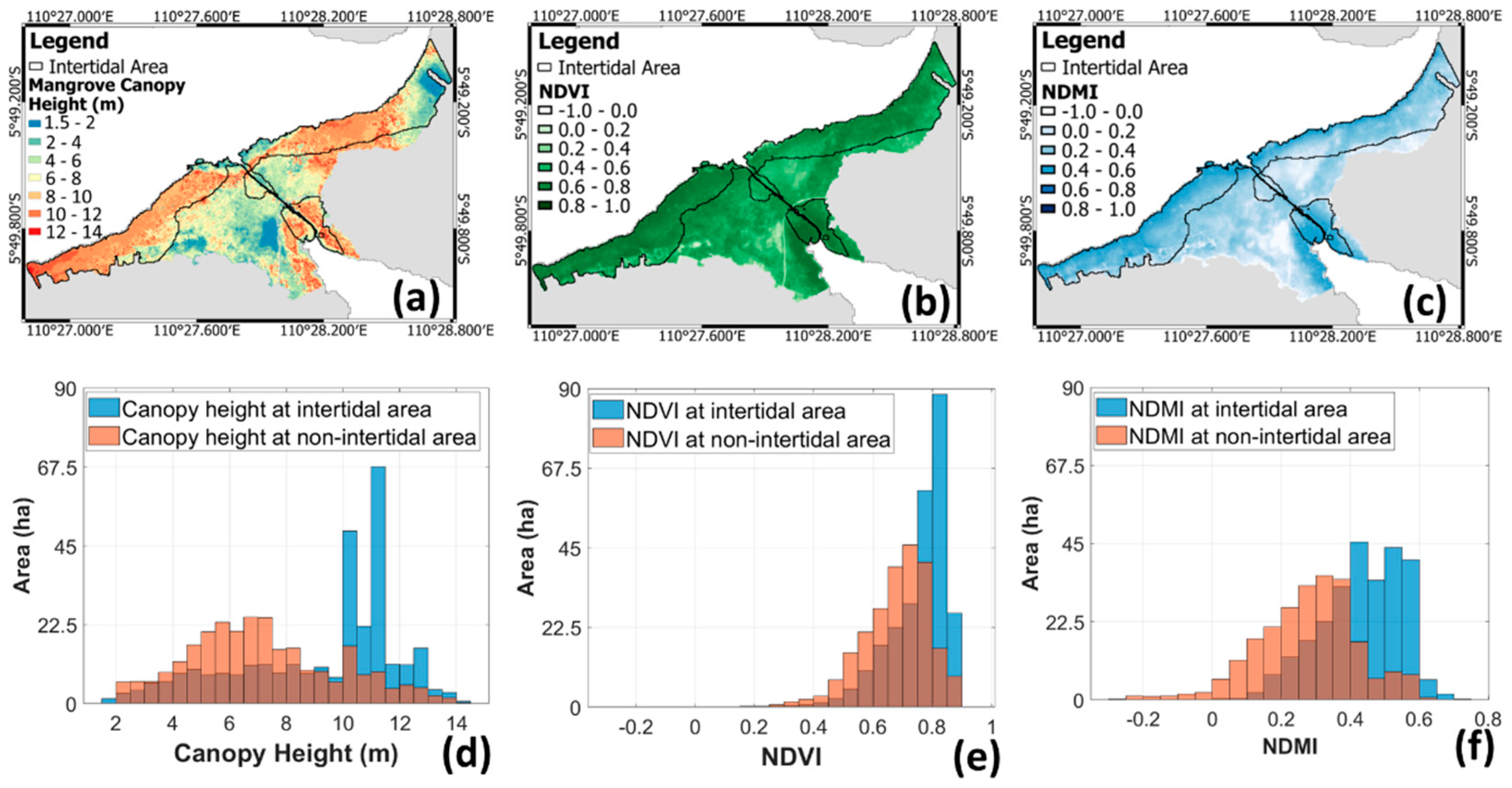
3.1. Vegetation Indices and Canopy Height in Intertidal and Non-Intertidal Area

The tidal analysis showed that the amplitudes of the tidal harmonic components of M2, O1, and K1 were 0.0434 m, 0.0893 m, and 0.2233 m, respectively. The tidal type in the KNP is mixed-tide prevailing diurnal [57]. This condition caused the intertidal area to be inundated by seawater once daily. Tides at KNP have the highest amplitude at the spring tide, reaching 0.6 m, whereas the MHHW is 0.4 m from the mean level. The average time of inundation in the intertidal areas is approximately 12 h per day. Not all intertidal areas have these inundation times; it depends on the tidal amplitude and topography of the intertidal area. Areas with high topography are inundated for shorter periods than areas with low topography. Figure 3 shows the intertidal area based on the calculations of MHHW and DTM.
The canopy height of mangroves (Figure 4a) at the fringe of the coastal area is taller than that in the middle area of the KNP and landward. When the mangrove canopy height is overlaid with the intertidal area, it is obvious that the tall mangroves are dominant in the intertidal area. The histogram of canopy height (Figure 4d) shows that the dominant mangroves in the intertidal area have a height of 10–11 m, with the total area being 138.7 ha. In comparison, the dominant mangroves in non-intertidal areas have a height of 5.5–7 m, with the total area being 92.8 ha.
Vegetation indices also show the same pattern as canopy height. It suggests that forest canopy closure influence NDVI and NDMI because tall vegetation has dense canopy closure [20] which means has greener and moist leaves. NDVI (Figure 4b) and NDMI (Figure 4c) in the fringe of coastal areas and intertidal areas have higher values than those in non-intertidal areas. NDVI in the intertidal area is dominated by NDVI 0.75–0.85 with a total area of 149.6 ha, while for non-intertidal areas, it is dominated by NDVI 0.65–0.8, with a total area of 126.3 ha (Figure 4e). In addition, NDMI in the intertidal area is dominated by NDMI 0.4–0.6, with a total area of 163.9 ha, while the non-intertidal area is dominated by NDMI 0.25–0.4 with a total area of 103.2 ha (Figure 4f). These results indicate that the intertidal area is greener and has higher humidity than the non-intertidal area. The sampling points in the intertidal area are F1, F2, S, N, T1, and T2, whereas those in the non-intertidal area are M1, M2, L1, and L2.

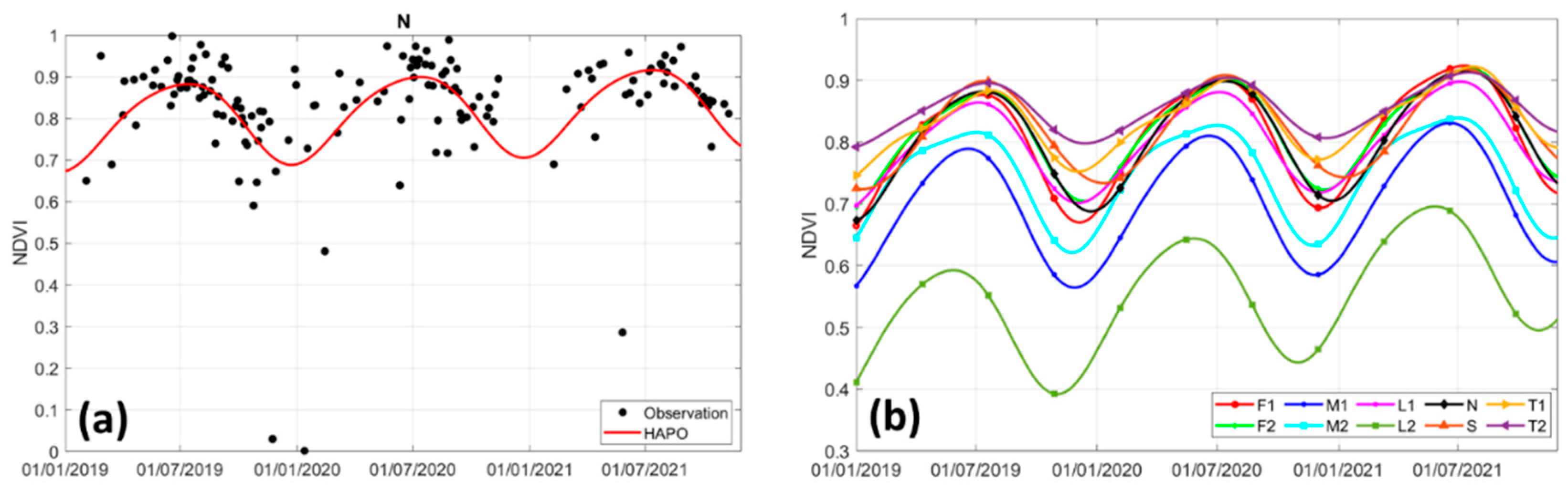
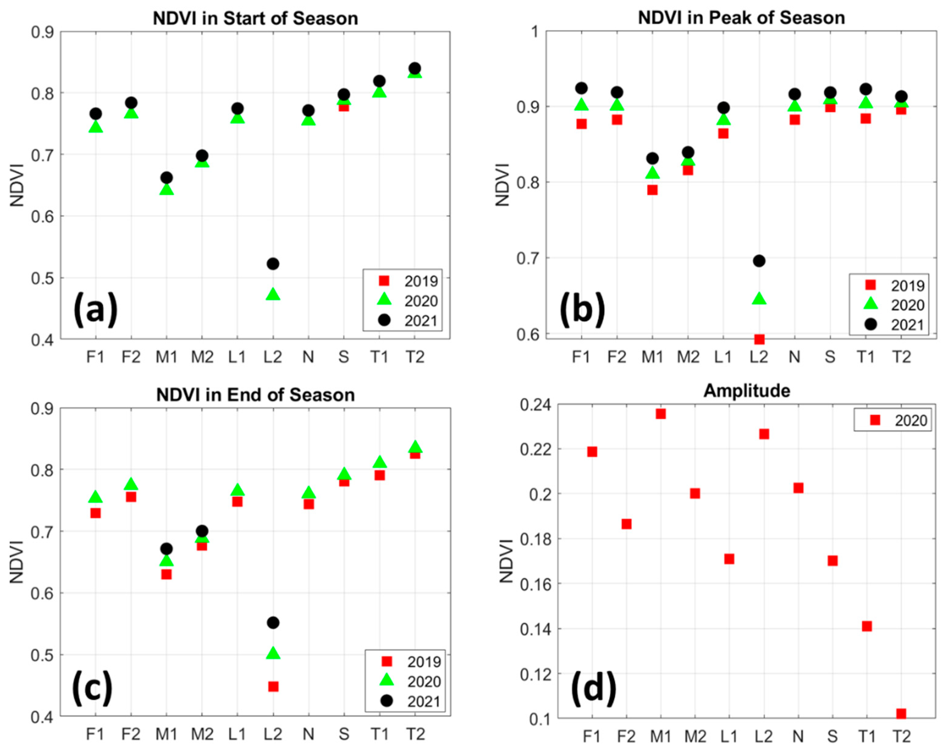
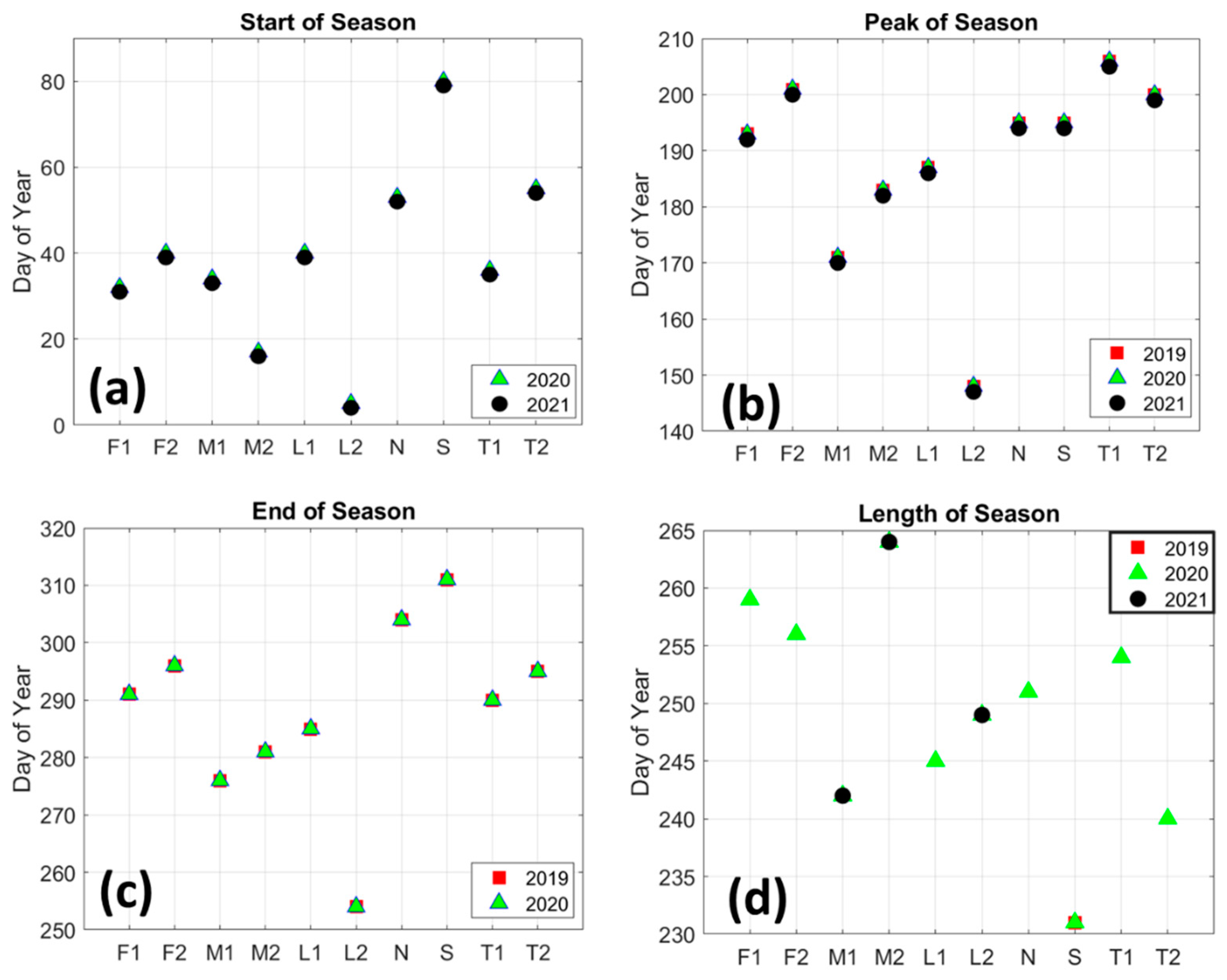
3.2. Mangrove Greenness Phenology

The harmonic regression results of the NDVI data using the HAPO method show a sinusoidal pattern that forms peaks and troughs (Figure 5a and Figure S1). The results of this HAPO fitting have an RMSE range of 0.05–0.09 and a correlation coefficient range of 0.5–0.9 compared to the median filtered NDVI data (Table 1). This error is relatively small and has a good correlation with the data. Therefore, we used the results of this HAPO regression to determine the phenological metrics in the KNP.
The harmonic regression results of NDVI for all observation points (Figure 5b) show that mangroves in the area east of the road (T2, T1), southern area (S), Northern area (N), shoreline area (F2, F1), and landward area north of the strait (L1) have higher NDVI values than at landward area south of the strait (L2), and middle area (M1, M2). These results are supported by the NDVI value at the POS (Figure 6b, Table S3) at the area east of the road (T2, T1), southern area (S), northern area (N), shoreline area (F2, F1), and the landward area north of strait (L1) ranging from 0.87–0.89, while the landward area south of the strait (L2), and middle area (M1, M2) range from 0.59–0.84. In addition, the NDVI for SOS (Figure 6a, Table S2) and EOS (Figure 6c, Table S4) show the same pattern. The NDVI at the area east of road (T2, T1), southern area (S), northern area (N), shoreline area (F2, F1), and the landward area north of the strait (L1) ranges from 0.74–0.84 at the SOS and from 0.73–0.83 at the EOS. At the landward area south of the strait (L2) and middle area (M1, M2), the NDVI ranges from 0.47–0.69 at the SOS and 0.44–0.69 at the EOS.
Furthermore, the AOS (Figure 6d, Table S5) at the area east of road (T2, T1), southern area (S), northern area (N), shoreline area (F2, F1), and the landward area north of strait (L1) ranges from 0.1–0.22, while at the landward area south of strait (L2), and middle area (M1, M2) ranges from 0.2–0.23. These AOS results indicate overlapping values that are not well discriminated against. It is noticeable that the AOS at points shoreline area north of strait (F1) and northern area (N) in the intertidal area are in the range of landward area south of strait (L2), and middle area (M1, M2) in the non-intertidal area. Moreover, mangrove in the landward area north of the strait (L1) has a low AOS, even though it is in the non-intertidal area. However, the NDVI in the shoreline area north of strait (F1) and northern area (N) remains higher than that in the landward area south of strait (L2) and middle area (M1, M2).
The NDVI at the SOS in 2020 has a lower value than that in 2021 (Figure 6a). In addition, the NDVI of the POS shows an increasing pattern from 2019 to 2021 (Figure 6b). The NDVI also shows the same pattern at the EOS (Figure 6c), where the NDVI in 2019 is lower than the NDVI in 2020. The SOS (Figure 7a, Table S6) occurs on the day of year (DOY) 4–80 (4 January–21 March), with the average being DOY 38 (February 7). the landward area south of the strait (L2) and the middle area south of the strait (M2), which are greening earlier than the other area, while southern area (S) is the latest. On the other hand, POS (Figure 7b, Table S7) occurs on DOY 147–206 (28 May–25 July), with the average being DOY 187 (July 5). The middle area north of the strait (M1) and the landward area south of the strait (L2) reach maximum greenness earlier than the others.
Furthermore, the EOS (Figure 7c, Table S8) occurs in the range of DOY 253–313 (10 September–7 November), with an average of DOY 289 (15 October). The landward area south of the strait (L2) ends its greenness earlier than the others. Thus, this area experiences an earlier SOS, POS, and EOS than other places. The LOS (Figure 7d, Table S9) ranges from 231–265 days, with an average of 249 days. The southern area (S) has the shortest green season, whereas the middle area south of the strait (M2) has the longest.

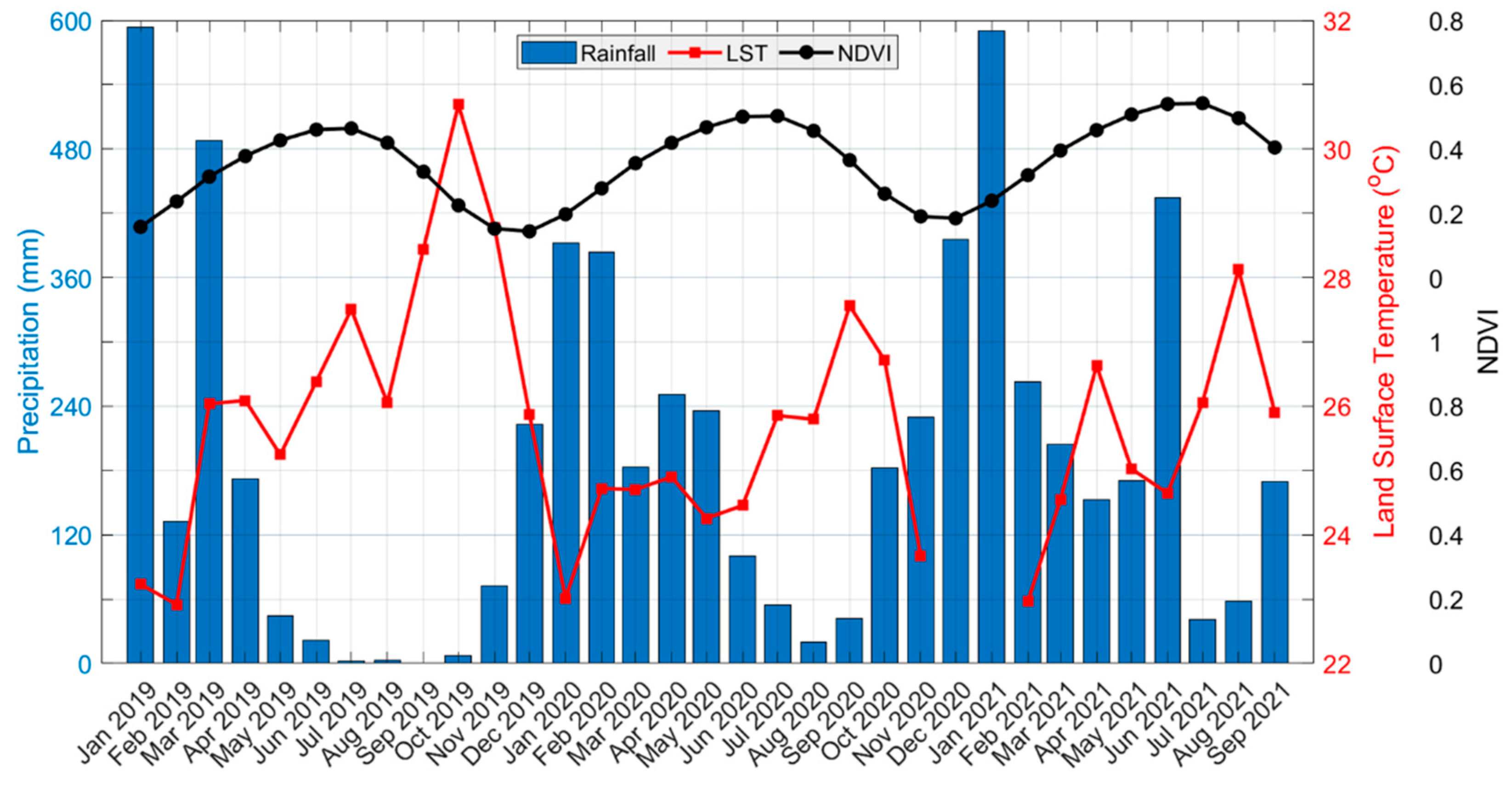
3.3. Rainfall and LST Variability Relationship with NDVI

The cross-correlation results between rainfall time series data and NDVI in KNP show a good correlation, with a correlation coefficient of 0.75 and a time lag of three months. This means that the maximum greenness of mangroves in the KNP occurs three months after high rainfall. High rainfall in KNP occurs from January to April, whereas the maximum greenness of mangroves occurs from May to July (Figure 8). The bar chart of rainfall (Figure 8) in 2019 shows a low rainfall, especially during the dry season (July–October), then it increased in 2020, and 2021 with an annual rate was 1761.3 mm in 2019 and 2468.8 mm in 2020. While the cumulation rainfall from January–September 2021 was 2084.5 mm. Thus, it indicates that the rainfall in KNP is varied annually, and it is likely influenced by the climate variability in Indonesia, e.g., monsoon, Indian Dipole Mode (IOD), and the El Niño-Southern Oscillation (ENSO) [58,59].
However, the cross-correlation results between LST and NDVI show a good correlation, with a correlation coefficient of 0.99 with no time lag. This indicates that NDVI is consistent with LST changes. The LST depends on the amount of solar radiation that an area receives [60] and solar radiation is an important parameter that influences plant growth and development via photosynthesis [61]. The LST in KNP does not exhibit extreme annual changes and only ranges from 23–30 °C (Figure 8).

4. Discussion

Studies on the effect of natural factors due to rainfall and tides on the sustainability of mangroves in KNP have not yet been found. The study by Puryono and Suryanti [12] remarked that mangrove deterioration was caused by human activities such as mangrove clearing for aquaculture, ponds, and tourism facilities. In addition, the study by Kamal et al. [11] and Latifah et al. [62] stated the possibility of natural factors influencing the degradation of mangroves. However, these studies did not explain what and how natural factors influence the degradation of mangroves. Here, we show that rainfall and tidal inundation as natural factors influence the greenness of mangroves in KNP. The greenness of the mangroves calculated using NDVI from the Sentinel-2 satellite can show the level of mangrove health. A green mangrove represents a dense green canopy, while a less green mangrove indicates a less canopy and dry leaves. We used tidal inundation mapping and phenology of mangrove greenness to demonstrate the influence of rainfall and tidal inundation on mangrove greenness. Unfortunately, we did not find any literature on research using the same method applied in KNP.
The map of the tidal inundation area (Figure 3) shows that not all mangrove areas are inundated by the tides. Therefore, we divided the area in this KNP into an intertidal area and a non-intertidal area. The intertidal area is 118.36 ha, and the non-intertidal area is 130.86 ha; thus, the non-intertidal area is wider than the intertidal. It is because the tidal range in the KNP is small, which is 1.2 m, with a maximum amplitude of only 0.6 m. The DTM data, as described in Section 2.3, has high accuracy since it has an RMSE of 0.008 m. It is relevant to a study by Kung et al. [63] that states that the accuracy of drone photogrammetry with GCPs ranges from 0.056 m to 1.25 m. Although the DTM spatial resolution is 15 m, we used this data because the topography in KNP is relatively flat.
The rainfall data we used may be inaccurate due to its low spatial resolution. However, the study by Prihantono et al. [18] showed that the GPM rainfall data in KNP compared to the observation data at the nearest meteorological station have a good correlation with RMSE = 92.39 mm/month and r = 0.93. Observational data is better to be used, but satellite data with small errors to nearby observation data can be used in this study when we do not find it. The LST data from MODIS was used in this study even though it has a spatial resolution of 1000 m because it still covers the study area with a total area of 22.19 km2, and the spatial resolution discrepancy of LST in this area is not so high. We want the spatial accuracy of the data as well as the Sentinel-2 spatial resolution (10 m). LST and rainfall have rough spatial resolution compared to NDVI, NDMI, and mangrove canopy height. Nevertheless, LST and rainfall data we used in this study have a slight discrepancy in the study area. Therefore, we can assume the rainfall and LST in the study area are constant spatially. The study by Wenbin et al. [64] showed that the LST data from MODIS has sufficient accuracy in representing the daily minimum air temperature with RMSE = 7.45 °C, MAE = 6.21°C, and r = 0.83.
We used three years of time-series data of Sentinel-2 images (2019–2021) to analyze the mangrove greenness phenology in KNP. The study by Songsom et al. [25] and Mandal et al. [28] used time-series data of vegetation index from MODIS for 10–18 years to analyze the phenology of mangrove forests. This data may determine the phenology well because of the long time-series data. However, this data cannot determine the phenology of mangrove zoning, which requires a high spatial resolution, especially in KNP, which has a small area. It is because the spatial resolution of the vegetation index in MODIS is 250 m and cannot distinguish well the mangrove zone. In contrast, the study by Li et al. [46] used Sentinel-2 for two years of time-series data to analyze the phenology-based classification of mangrove species in the Zhangjiang River estuary, China. Since our study aimed to analyze the phenology of mangrove zonation in KNP, we chose to use Sentinel-2, which has a good temporal and spatial resolution.
Based on the histogram of extraction pixel of the intertidal area and non-intertidal area (Figure 4), it was evident that tall mangroves, high NDVI, and high NDMI dominate the intertidal area. In contrast, the non-intertidal zone is dominated by short mangroves, low NDVI, and low NDMI values. This shows that the intertidal area is dominated by taller, greener, healthier mangroves and a moister substrate than the non-intertidal area. This pattern is commonly found in mangrove ecosystems that experience seaward fringing. In intertidal areas, mangroves tend to be taller than those with high topography and limited tidal inundation [65,66]. A study by Bathman et al. [67] showed that coastal areas that are frequently flooded by tides tend to be dominated by higher mangrove species than areas that are rarely or not flooded by tides. Differences in the height of mangroves occur because of species distribution, in which zones of growth occur as an adaptation to different environmental factors [68] that depend on tidal inundation regimes [67,69,70]. These are related to nutrient availability [71], porewater salinity [72,73], freshwater inputs, interplay with geomorphology [74], and biotic factors, such as competition for resources [75]. Based on observational data from BTNKJ [31,32], Rhizophora sp. is the dominant mangrove species around the seafront in KNP, which is usually inundated by the tide. Meanwhile, the middle area of KNP, which is not flooded by tidal, is dominated by Ceriops tagal and Lumnitzera sp. According to Alongi [76], Rhizophora sp. is a species of mangrove that usually grows in low to medium elevation intertidal areas with medium to high salinity. In contrast, Ceriops tagal and Lumnitzera sp. are mangrove species that grow in high elevation intertidal areas with very high salinity.
Intertidal areas periodically inundated by tidal movements tend to have healthier and taller mangroves because tides dilute the salinity, re-establishing suitable temperatures and oxygen levels in the intertidal region [77]. Salt accumulation in soil porewater is diluted and washed away by the tides [78]. Meanwhile, pore water salinity in the non-intertidal or high intertidal zone is usually higher than in the lower intertidal zone because of the limited inundation that flushes out salt and strong evapotranspiration due to high temperatures and low rainfall [79]. This condition usually occurs during the dry season when the soil moisture and the water table in KNP are lower than the average [18]. The high salinity of the pore water in the non-intertidal zone causes mangrove growth to decrease due to low water uptake and decreased transpiration and photosynthesis [72,80]. During the dry season, the salinity in non-intertidal areas in KNP was higher than that in intertidal areas. According to a study by Hudoyo et al. [57], surface groundwater salinity in KNP ranges from 43–51 ppt during the dry season. Thus, tides play a very important role in the growth, health, and greenness of mangroves.
One of the impacts of climate change is the rise in sea level. This phenomenon causes coastal areas and small islands to be inundated and experience a decline in the area. The Intergovernmental Panel on Climate Change (IPCC) forecasts that mangrove regions will start to grow closer to the polar regions and will likely continue to survive in the future along with rising global temperatures, sea levels, and atmospheric CO2 concentrations. In addition, mangroves might grow landward as inundation expands due to sea-level rise, which might positively impact mangrove greenness. However, the zonation of mangroves may change and become dominated by species that can adapt to high salinity. Numerical simulation by Teh et al. [81] showed the shift of mangroves to the landward as the increase in groundwater salinity to the landward due to the sea level rise. It is because mangroves can adapt to saline areas compared to land vegetations.
The AOS (Figure 6d) in the intertidal area is lower than that in the non-intertidal area. This suggests that mangroves in the intertidal area are almost evergreen and less affected by rainfall limitations. Moreover, mangrove canopy cover and the heterogeneity of mangrove species may influence the seasonal amplitude in KNP. For example, the shoreline area north of the strait (F1), which is in the intertidal area, has a high AOS, whereas the landward area north of the strait (L1) has a low AOS, even though it is in a non-intertidal area. This may be because the mangrove canopy cover in the shoreline area north of the strait (F1) was less than that in the landward area north of the strait (L1) as an observation by Hudoyo et al. [57]. In addition, the northern area (N), which has a high AOS, may be caused by a mix of mangrove species with different canopy cover in this area. Furthermore, a high AOS indicates low mangrove coverage. For example, the naturally degraded landward area south of the strait (L2), dominated by dwarf mangroves and dieback as reported by Kamal et al. [11], has the lowest NDVI and the highest amplitude of the season.
The LST is positively correlated with NDVI because it coincides with the photosynthetic rate. It is proportional to the solar radiation [60] received by vegetation, and vegetation is required for photosynthesis to grow and develop [61]. This suggests that the LST is not the main factor controlling greenness, with rainfall being the controlling factor. This result is consistent with a study conducted by Songsom et al. [25] that rainfall was the only driver that showed a positive relationship for all sites of mangrove forest in Southern Thailand compared to temperature and solar radiation.
Rainfall affects the greenness and health of mangroves in KNP. The mangrove greenness phenology in KNP shows that the maximum greenness of mangroves occurs in the summer around July every year after the rainy season and the lowest greenness of mangrove occurs at the end of the dry season (October–November) every year (Section 3.3). In addition, the NDVI of mangroves in 2019 was low, and then it rose with an increase in annual rainfall. This indicates that mangrove greenness is strongly influenced by rainfall. On the other hand, the climate in Indonesia is influenced by climate variabilities such as the monsoon, IOD, and the ENSO. Thus, the greenness of mangroves in KNP is also influenced by climate variability. For example, rainfall in 2019 was low, which may have been caused by the coincidence of the east monsoon, El Niño, and positive IOD conditions. It is based on the study by Ramadhan et al. [82] that showed indications of El Niño and positive IOD indicated by the cooling effect of sea surface temperatures and the thinning of the thermocline layer on the southern coast of Java in 2019. Due to mangrove greenness in KNP being influenced by climate variability, it is likely the mangrove in KNP also vulnerable to drought. Therefore, it is possible to apply the drought index that incorporates rainfall, LST, and vegetation index to assess and monitor mangrove health due to drought in KNP after the study by Alahacoon et al. [41,83].
Rainfall is a source of freshwater in the KNP. Mangroves require freshwater for growth. Rainwater can dilute the salt and decrease pore water salinity, thereby increasing water uptake and nutrient adsorption in the soil by mangroves. During the rainy season, rainwater inundates the mangrove substrate in the KNP [18]. Under these wet conditions, the mangrove substrate may provide nutrients in non-intertidal areas [84,85]. Rainfall plays a major role in the greenness phenology of mangroves in KNP because it has a positive and high correlation coefficient with NDVI (Section 3.3). Mangroves in KNP begin to green around February and reach a peak of greenness around July, with their greenery diminishing around October (Section 3.2). Thus, the optimal absorption of carbon by mangroves in the atmosphere in KNP occurs from February to October, with the maximum absorption occurring in July. This finding shows that mangroves in Karimunjawa can compensate for the release of CO2 by the Java Sea, which peaks during the first transitional season around April–May, according to the study of Wirasatriya et al. [9].

5. Conclusions

This study demonstrated that the intertidal area is dominated by tall mangroves, high NDVI, high soil moisture, and vice versa. Rainfall positively correlates with NDVI in the intertidal and non-intertidal areas, although the impact on the intertidal area is lower than that in the non-intertidal area. It suggests that mangroves in the intertidal areas are almost evergreen. LST is not likely the main control of mangrove greenness because it correlates positively with the photosynthetic rate and is required to assist vegetation in growing and developing. The analysis of mangrove greenness phenology indicates that mangroves in the KNP have optimal greenness from February to October, with maximum greenness in July. Therefore, optimal carbon sequestration in those months may occur in the KNP. Thus, we can conclude that rainfall and tidal inundation markedly affect the mangrove greenness in the KNP. Rainfall and tidal inundation may control soil salinity, which affects mangrove species distribution, salt dilution in the mangrove zone, lowering soil temperature, and increasing soil moisture and nutrients.
However, further research is required to analyze the nutrient and salinity characteristics of mangrove substrates in KNP. It suggests that mangroves in the KNP are vulnerable to climate variability and climate change that limit rainfall. Therefore, a study of drought and vegetation health in the long-term data also should be conducted. Furthermore, future sea-level rise due to climate change might positively impact mangrove greenness in KNP, even though mangrove zonation will change and be dominated by mangrove species that can adapt to high salinity. Therefore, the government, stakeholders, and communities in Karimunjawa and Kemujan Island should actively conserve the mangrove regions because, besides anthropogenic factors, mangroves in Karimunjawa and Kemujan Island are vulnerable to natural factors, particularly those in the non-intertidal area.

Supplementary Materials

The following supporting information can be downloaded at: https://www.mdpi.com/article/10.3390/su14148948/s1, Figure S1: Harmonic regression using the HAPO method on scattered NDVI time-series data at point F1, F2, M1, M2, L1, L2, N, S, T1, and T2 from 1 January 2019–31 December 2021; Table S1: Dataset of Sentinel-2 L2A in KNP area used in this study; Table S2: NDVI at SOS for each sampling point; Table S3: NDVI at POS for each sampling point; Table S4: NDVI at EOS for each sampling point; Table S5: AOS for each sampling point; Table S6: SOS, average SOS for each sampling point, and Temporal average SOS in 2019, 2020, and 2021; Table S7: POS, average POS for each sampling point, and Temporal average POS in 2019, 2020, and 2021; Table S8: EOS, average EOS for each sampling point, and Temporal average EOS in 2019, 2020, and 2021; Table S9: LOS, average LOS for each sampling point, and Temporal average LOS in 2019, 2020, and 2021.

Author Contributions

Conceptualization, J.P. and T.N.; methodology, J.P. and T.N.; software, J.P.; validation, J.P., A.W. and T.N.; formal analysis, J.P. and T.N.; investigation, J.P., A.W. and T.N.; resources, J.P. and A.W.; data curation, J.P. and A.W.; writing—original draft preparation, J.P.; writing—review and editing, J.P., A.W. and T.N.; visualization, J.P.; supervision, T.N. and K.N.; project administration, N.S.A. and K.N.; funding acquisition, K.N. All authors have read and agreed to the published version of the manuscript.

Funding

This study was funded by Japan Science and Technology Agency (JST) and Japan International Cooperation Agency (JICA) through the Science and Technology Research Partnership for Sustainable Development (SATREPS) program through the “Comprehensive Assessment and Conservation of Blue Carbon Ecosystem and their Services in the Coral Triangle (BlueCARES)” Project.

Institutional Review Board Statement

Not applicable.

Informed Consent Statement

Not applicable.

Data Availability Statement

The data is available at https://figshare.com/s/8e69518850c5a046e5be (accessed on 25 May 2022).

Acknowledgments

We would like to thank the Faculty of Fisheries and Marine Sciences, Diponegoro University, for the data support in this study.

Conflicts of Interest

The authors declare no conflict of interest. The funders had no role in the design of the study; in the collection, analyses, or interpretation of data; in the writing of the manuscript, or in the decision to publish the results.

References

  1. Alongi, D.M. Carbon Sequestration in Mangrove Forests. Carbon Manag. 2012, 3, 313–322. [Google Scholar] [CrossRef]
  2. Alongi, D.M. Global Significance of Mangrove Blue Carbon in Climate Change Mitigation (Version 1). Science 2020, 2, 57. [Google Scholar] [CrossRef]
  3. Donato, D.C.; Kauffman, J.B.; Murdiyarso, D.; Kurnianto, S.; Stidham, M.; Kanninen, M. Mangroves among the Most Carbon-Rich Forests in the Tropics. Nat. Geosci. 2011, 4, 293–297. [Google Scholar] [CrossRef]
  4. Kauffman, J.B.; Bernardino, A.F.; Ferreira, T.O.; Giovannoni, L.R.; De Gomes, L.E.O.; Romero, D.J.; Jimenez, L.C.Z.; Ruiz, F. Carbon Stocks of Mangroves and Salt Marshes of the Amazon Region, Brazil. Biol. Lett. 2018, 14, 20180208. [Google Scholar] [CrossRef]
  5. Chiodi, A.M.; Dunne, J.P.; Harrison, D.E. Estimating Air-Sea Carbon Flux Uncertainty over the Tropical Pacific: Importance of Winds and Wind Analysis Uncertainty. Glob. Biogeochem. Cycles 2019, 33, 370–390. [Google Scholar] [CrossRef]
  6. Kartadikaria, A.R.; Watanabe, A.; Nadaoka, K.; Adi, N.S.; Prayitno, H.B.; Soemorumekso, S.; Muchtar, M.; Triyulianti, I.; Setiawan, A.; Suratno, S.; et al. CO2 Sink/Source Characteristics in the Tropical Indonesian Seas. J. Geophys. Res. Ocean. 2015, 120, 7842–7856. [Google Scholar] [CrossRef] [Green Version]
  7. Sidik, F.; Supriyanto, B.; Krisnawati, H.; Muttaqin, M.Z. Mangrove Conservation for Climate Change Mitigation in Indonesia. Wiley Interdiscip. Rev. Clim. Chang. 2018, 9, e529. [Google Scholar] [CrossRef]
  8. Murdiyarso, D.; Purbopuspito, J.; Kauffman, J.B.; Warren, M.W.; Sasmito, S.D.; Donato, D.C.; Manuri, S.; Krisnawati, H.; Taberima, S.; Kurnianto, S. The Potential of Indonesian Mangrove Forests for Global Climate Change Mitigation. Nat. Clim. Chang. 2015, 5, 1089–1092. [Google Scholar] [CrossRef]
  9. Wirasatriya, A.; Sugianto, D.N.; Maslukah, L.; Ahkam, M.F.; Wulandari, S.Y.; Helmi, M. Carbon Dioxide Flux in the Java Sea Estimated from Satellite Measurements. Remote Sens. Appl. Soc. Environ. 2020, 20, 100376. [Google Scholar] [CrossRef]
  10. Latifah, N.; Febrianto, S.; Wirasatriya, A.; Endrawati, H.; Zainuri, M.; Suryanti, S.; Hidayat, A.N. Air-Sea Flux of CO2 In the Waters of Karimunjawa Island, Indonesia. Saintek Perikan. Indones. J. Fish. Sci. Technol. 2020, 16, 171–178. [Google Scholar] [CrossRef]
  11. Kamal, M.; Hartono, H.; Wicaksono, P.; Adi, N.S.; Arjasakusuma, S. Assessment of Mangrove Forest Degradation Through Canopy Fractional Cover in Karimunjawa Island, Central Java, Indonesia. Geoplan. J. Geomatics Plan. 2016, 3, 107. [Google Scholar] [CrossRef] [Green Version]
  12. Puryono, S.; Suryanti, S. Degradation of Mangrove Ecosystem in Karimunjawa Island Based on Public Perception and Management. In Proceedings of the IOP Conference Series: Earth and Environmental Science, Moscow, Russia, 27 May–6 June 2019; Volume 246. [Google Scholar]
  13. Kanniah, K.D.; Kang, C.S.; Sharma, S.; Aldrie Amir, A. Remote Sensing to Study Mangrove Fragmentation and Its Impacts on Leaf Area Index and Gross Primary Productivity in the South of Peninsular Malaysia. Remote Sens. 2021, 13, 1427. [Google Scholar] [CrossRef]
  14. Alongi, D.M. The Impact of Climate Change on Mangrove Forests. Curr. Clim. Chang. Rep. 2015, 1, 30–39. [Google Scholar] [CrossRef]
  15. Santini, N.S.; Reef, R.; Lockington, D.A.; Lovelock, C.E. The Use of Fresh and Saline Water Sources by the Mangrove Avicennia Marina. Hydrobiologia 2015, 745, 59–68. [Google Scholar] [CrossRef]
  16. Chamberlain, D.A.; Phinn, S.R.; Possingham, H.P. Mangrove Forest Cover and Phenology with Landsat Dense Time Series in Central Queensland, Australia. Remote Sens. 2021, 13, 3032. [Google Scholar] [CrossRef]
  17. Hayes, M.A.; Jesse, A.; Welti, N.; Tabet, B.; Lockington, D.; Lovelock, C.E. Groundwater Enhances Above-Ground Growth in Mangroves. J. Ecol. 2019, 107, 1120–1128. [Google Scholar] [CrossRef]
  18. Prihantono, J.; Adi, N.S.; Nakamura, T.; Nadaoka, K. The Impact of Groundwater Variability on Mangrove Greenness in Karimunjawa National Park Based on Remote Sensing Study. In Proceedings of the IOP Conference Series: Earth and Environmental Science, Jakarta, Indonesia, 25–26 September 2021; Volume 925. [Google Scholar]
  19. Saleh, M.B.; Dewi, R.W.; Prasetyo, L.B.; Santi, N.A. Canopy Cover Estimation in Lowland Forest in South Sumatera, Using LiDAR and Landsat 8 OLI Imagery. J. Manaj. Hutan Trop. 2021, 27, 50–58. [Google Scholar] [CrossRef]
  20. Ansley, R.J.; Mirik, M.; Surber, B.W.; Park, S.C. Canopy Area and Aboveground Mass of Individual Redberry Juniper (Juniperus pinchotii) Trees. Rangel. Ecol. Manag. 2012, 65, 189–195. [Google Scholar] [CrossRef]
  21. Wang, L.; Jia, M.; Yin, D.; Tian, J. A Review of Remote Sensing for Mangrove Forests: 1956–2018. Remote Sens. Environ. 2019, 231, 111223. [Google Scholar] [CrossRef]
  22. Heumann, B.W. Satellite Remote Sensing of Mangrove Forests: Recent Advances and Future Opportunities. Prog. Phys. Geogr. 2011, 35, 87–108. [Google Scholar] [CrossRef]
  23. Pastor-Guzman, J.; Dash, J.; Atkinson, P.M. Remote Sensing of Mangrove Forest Phenology and Its Environmental Drivers. Remote Sens. Environ. 2018, 205, 71–84. [Google Scholar] [CrossRef] [Green Version]
  24. Xu, R.; Zhao, S.; Ke, Y. A Simple Phenology-Based Vegetation Index for Mapping Invasive Spartina Alterniflora Using Google Earth Engine. IEEE J. Sel. Top. Appl. Earth Obs. Remote Sens. 2021, 14, 190–201. [Google Scholar] [CrossRef]
  25. Songsom, V.; Koedsin, W.; Ritchie, R.J.; Huete, A. Mangrove Phenology and Environmental Drivers Derived from Remote Sensing in Southern Thailand. Remote Sens. 2019, 11, 955. [Google Scholar] [CrossRef] [Green Version]
  26. Matongera, T.N.; Mutanga, O.; Sibanda, M.; Odindi, J. Estimating and Monitoring Land Surface Phenology in Rangelands: A Review of Progress and Challenges. Remote Sens. 2021, 13, 2060. [Google Scholar] [CrossRef]
  27. Reed, B.C.; Brown, J.F.; VanderZee, D.; Loveland, T.R.; Merchant, J.W.; Ohlen, D.O. Measuring Phenological Variability from Satellite Imagery. J. Veg. Sci. 1994, 5, 703–714. [Google Scholar] [CrossRef]
  28. Mandal, M.S.H.; Kamruzzaman, M.; Hosaka, T. Elucidating the Phenology of the Sundarbans Mangrove Forest Using 18-Year Time Series of MODIS Vegetation Indices. Tropics 2020, 29, 41–55. [Google Scholar] [CrossRef]
  29. Tang, J.; Körner, C.; Muraoka, H.; Piao, S.; Shen, M.; Thackeray, S.J.; Yang, X. Emerging Opportunities and Challenges in Phenology: A Review. Ecosphere 2016, 7, e01436. [Google Scholar] [CrossRef] [Green Version]
  30. Mulyadi, H.; Susanto, H.; Devi, Y.; Sahwan, F.F. Interpretation of Mangrove Trekking Karimunjawa National Park, 2nd ed.; Karimunjawa National Park Office (BTNKJ): Semarang, Indonesia, 2019. [Google Scholar]
  31. Balai Taman Nasional Karimunjawa (BTNKJ). Report of Mangrove Inventory at Karimunjawa Island; Balai Taman Nasional Karimunjawa (BTNKJ): Semarang, Indonesia, 2013. [Google Scholar]
  32. Balai Taman Nasional Karimunjawa (BTNKJ). Report of Mangrove Inventory at Kemujan Island; Balai Taman Nasional Karimunjawa (BTNKJ): Semarang, Indonesia, 2013. [Google Scholar]
  33. Wirasatriya, A.; Pribadi, R.; Iryanthony, S.B.; Maslukah, L.; Sugianto, D.N.; Helmi, M.; Ananta, R.R.; Adi, N.S.; Kepel, T.L.; Ati, R.N.A.; et al. Mangrove Above-Ground Biomass and Carbon Stock in the Karimunjawa-Kemujan Islands Estimated from Unmanned Aerial Vehicle-Imagery. Sustainability 2022, 14, 706. [Google Scholar] [CrossRef]
  34. Huffman, G.J.; Stocker, E.F.; Bolvin, D.T.; Nelkin, E.J.; Tan, J. GPM IMERG Final Precipitation L3 1 Month 0.1 Degree x 0.1 Degree V06, Greenbelt, MD. Available online: https://disc.gsfc.nasa.gov/datasets/GPM_3IMERGM_06/summary (accessed on 28 February 2022).
  35. Wan, Z. Collection-6 MODIS Land Surface Temperature Products Users’ Guide; ERI, University of California: Santa Barbara, CA, USA, 2013. [Google Scholar]
  36. Kriegler, F.; Malila, W.; Nalepka, R.; Richardson, W. Preprocessing Transformations and Their Effect on Multispectral Recognition. In Proceedings of the 6th International Symposium on Remote Sensing of Environment, Ann Arbor, MI, USA, 13–16 October 1969; University of Michigan: Ann Arbor, MI, USA, 1969; pp. 97–131. [Google Scholar]
  37. Rouse, J.W.; Haas, R.H.; Schell, J.A.; Deering, D.W. Monitoring Vegetation Systems in the Great Plains with ERTS. In Proceedings of the Third Earth Resources Technology Satellite-1 Symposium, Washington, DC, USA, 10–14 December 1974; Greenbelt, NASA SP-351. pp. 48–62. [Google Scholar]
  38. Wilson, E.H.; Sader, S.A. Detection of Forest Harvest Type Using Multiple Dates of Landsat TM Imagery. Remote Sens. Environ. 2002, 80, 385–396. [Google Scholar] [CrossRef]
  39. Zhang, X.; Treitz, P.M.; Chen, D.; Quan, C.; Shi, L.; Li, X. Mapping Mangrove Forests Using Multi-Tidal Remotely-Sensed Data and a Decision-Tree-Based Procedure. Int. J. Appl. Earth Obs. Geoinf. 2017, 62, 201–214. [Google Scholar] [CrossRef]
  40. Gao, B.C. NDWI—A Normalized Difference Water Index for Remote Sensing of Vegetation Liquid Water from Space. Remote Sens. Environ. 1996, 58, 257–266. [Google Scholar] [CrossRef]
  41. Alahacoon, N.; Edirisinghe, M. A Comprehensive Assessment of Remote Sensing and Traditional Based Drought Monitoring Indices at Global and Regional Scale. Geomat. Nat. Hazards Risk 2022, 13, 762–799. [Google Scholar] [CrossRef]
  42. Intergovernmental Committee on Surveying and Mapping (ICSM). Australian Tides Manual Special Publication No. 9; Intergovernmental Committee on Surveying and Mapping (ICSM): Canberra, Australia, 2021.
  43. Pawlowicz, R.; Beardsley, B.; Lentz, S. Classical Tidal Harmonic Analysis Including Error Estimates in MATLAB Using T_TIDE. Comput. Geosci. 2002, 28, 929–937. [Google Scholar] [CrossRef]
  44. Li, N.; Zhan, P.; Pan, Y.; Zhu, X.; Li, M.; Zhang, D. Comparison of Remote Sensing Time-Series Smoothing Methods for Grassland Spring Phenology Extraction on the Qinghai–Tibetan Plateau. Remote Sens. 2020, 12, 3383. [Google Scholar] [CrossRef]
  45. Zhou, J.; Jia, L.; Menenti, M.; Gorte, B. On the Performance of Remote Sensing Time Series Reconstruction Methods—A Spatial Comparison. Remote Sens. Environ. 2016, 187, 367–384. [Google Scholar] [CrossRef]
  46. Li, H.; Jia, M.; Zhang, R.; Ren, Y.; Wen, X. Incorporating the Plant Phenological Trajectory into Mangrove Species Mapping with Dense Time Series Sentinel-2 Imagery and the Google Earth Engine Platform. Remote Sens. 2019, 11, 2479. [Google Scholar] [CrossRef] [Green Version]
  47. Malamiri, H.R.G.; Zare, H.; Rousta, I.; Olafsson, H.; Verdiguier, E.I.; Zhang, H.; Mushore, T.D. Comparison of Harmonic Analysis of Time Series (HANTS) and Multi-Singular Spectrum Analysis (M-SSA) in Reconstruction of Long-Gap Missing Data in NDVI Time Series. Remote Sens. 2020, 12, 2747. [Google Scholar] [CrossRef]
  48. Zhou, J.; Jia, L.; Menenti, M.; Liu, X. Optimal Estimate of Global Biome—Specific Parameter Settings to Reconstruct Ndvi Time Series with the Harmonic Analysis of Time Series (Hants) Method. Remote Sens. 2021, 13, 4251. [Google Scholar] [CrossRef]
  49. Verhoef, W. Application of Harmonic Analysis of NDVI Time Series (HANTS). Fourier Anal. Temporal NDVI S. Afr. Am. Cont. 1996, 108, 19–24. [Google Scholar]
  50. Adams, B.; Iverson, L.; Matthews, S.; Peters, M.; Prasad, A.; Hix, D.M. Mapping Forest Composition with Landsat Time Series: An Evaluation of Seasonal Composites and Harmonic Regression. Remote Sens. 2020, 12, 610. [Google Scholar] [CrossRef] [Green Version]
  51. Mishra, N.B.; Crews, K.A.; Neuenschwander, A.L. Sensitivity of EVI-Based Harmonic Regression to Temporal Resolution in the Lower Okavango Delta. Int. J. Remote Sens. 2012, 33, 7703–7726. [Google Scholar] [CrossRef]
  52. Wilson, B.T.; Knight, J.F.; McRoberts, R.E. Harmonic Regression of Landsat Time Series for Modeling Attributes from National Forest Inventory Data. ISPRS J. Photogramm. Remote Sens. 2018, 137, 29–46. [Google Scholar] [CrossRef]
  53. Zhou, Q.; Zhu, Z.; Xian, G.; Li, C. A Novel Regression Method for Harmonic Analysis of Time Series. ISPRS J. Photogramm. Remote Sens. 2022, 185, 48–61. [Google Scholar] [CrossRef]
  54. Zhou, Q. Harmonic Adaptive Penalty Operator (HAPO): U.S. Geological Survey Software Release. Available online: https://code.usgs.gov/lcmap/research/Harmonic-Adaptive-Penalty-Operator-HAPO (accessed on 7 February 2022).
  55. White, M.A.; Thornton, P.E.; Running, S.W. A Continental Phenology Model for Monitoring Vegetation Responses to Interannual Climatic Variability. Glob. Biogeochem. Cycles 1997, 11, 217–234. [Google Scholar] [CrossRef]
  56. Garonna, I.; de Jong, R.; de Wit, A.J.W.; Mücher, C.A.; Schmid, B.; Schaepman, M.E. Strong Contribution of Autumn Phenology to Changes in Satellite-Derived Growing Season Length Estimates across Europe (1982–2011). Glob. Chang. Biol. 2014, 20, 3457–3470. [Google Scholar] [CrossRef]
  57. Hudoyo, F.; Widada, S.; Maslukah, L.; Rochaddi, B.; Wirasatriya, A.; Adi, N.S. Study of Tidal Analysis, Distribution of Brackish Groundwater and Sediments and Their Effect on Mangrove Distribution Patterns in the Karimunjawa Islands. Indones. J. Oceanogr. 2021, 3, 409–418. [Google Scholar] [CrossRef]
  58. Abram, N.J.; Gagan, M.K.; Cole, J.E.; Hantoro, W.S.; Mudelsee, M. Recent Intensification of Tropical Climate Variability in the Indian Ocean. Nat. Geosci. 2008, 1, 849–853. [Google Scholar] [CrossRef]
  59. Ummenhofer, C.C.; D’Arrigo, R.D.; Anchukaitis, K.J.; Buckley, B.M.; Cook, E.R. Links between Indo-Pacific Climate Variability and Drought in the Monsoon Asia Drought Atlas. Clim. Dyn. 2013, 40, 1319–1334. [Google Scholar] [CrossRef] [Green Version]
  60. Peng, X.; Wu, W.; Zheng, Y.; Sun, J.; Hu, T.; Wang, P. Correlation Analysis of Land Surface Temperature and Topographic Elements in Hangzhou, China. Sci. Rep. 2020, 10, 10451. [Google Scholar] [CrossRef]
  61. Tong, R.; Cao, Y.; Zhu, Z.; Lou, C.; Zhou, B.; Wu, T. Solar Radiation Effects on Leaf Nitrogen and Phosphorus Stoichiometry of Chinese Fir across Subtropical China. For. Ecosyst. 2021, 8, 62. [Google Scholar] [CrossRef]
  62. Latifah, N.; Febrianto, S.; Endrawati, H.; Zainuri, M. Mapping of Classification and Analysis of Changes in Mangrove Ecosystem Using Multi-Temporal Satellite Images in Karimunjawa, Jepara, Indonesia. J. Kelaut. Trop. 2018, 21, 97. [Google Scholar] [CrossRef]
  63. Küng, O.; Strecha, C.; Beyeler, A.; Zufferey, J.-C.; Floreano, D.; Fua, P.; Gervaix, F. The accuracy of automatic photogrammetric techniques on ultra-light UAV imagery. Int. Arch. Photogramm. Remote Sens. Spat. Inf. Sci. 2012, XXXVIII-1, 125–130. [Google Scholar] [CrossRef] [Green Version]
  64. Zhu, W.; Lu, A.; Jia, S. Estimation of Daily Maximum and Minimum Air Temperature Using MODIS Land Surface Temperature Products. Remote Sens. Environ. 2013, 130, 62–73. [Google Scholar] [CrossRef]
  65. Feller, I.C.; Lovelock, C.E.; Berger, U.; McKee, K.L.; Joye, S.B.; Ball, M.C. Biocomplexity in Mangrove Ecosystems. Ann. Rev. Mar. Sci. 2010, 2, 395–417. [Google Scholar] [CrossRef] [Green Version]
  66. Lugo, A.E. Mangrove Ecosystems: Successional or Steady State? Biotropica 1980, 12, 65. [Google Scholar] [CrossRef]
  67. Bathmann, J.; Peters, R.; Reef, R.; Berger, U.; Walther, M.; Lovelock, C.E. Modelling Mangrove Forest Structure and Species Composition over Tidal Inundation Gradients: The Feedback between Plant Water Use and Porewater Salinity in an Arid Mangrove Ecosystem: The Feedback between Plant Water Use and Porewater Salinity in an Arid. Agric. For. Meteorol. 2021, 308–309, 108547. [Google Scholar] [CrossRef]
  68. Dobbertin, M. Tree Growth as Indicator of Tree Vitality and of Tree Reaction to Environmental Stress: A Review. Eur. J. For. Res. 2005, 124, 319–333. [Google Scholar] [CrossRef]
  69. Ball, J.M.; James, R.D. Proposed Experimental Tests of a Theory of Fine Microstructure and the Two-Well Problem. Philos. Trans. R. Soc. Lond. Ser. A Phys. Eng. Sci. 1992, 338, 389–450. [Google Scholar] [CrossRef]
  70. Watson, J.G. Mangrove Forests of the Malay Peninsula; Malayan Forest Records; Fraser & Neave: Kuala Lumpur, Malaysia, 1928. [Google Scholar]
  71. Feller, I.C.; McKee, K.L.; Whigham, D.F.; O’Neill, J.P. Nitrogen vs. Phosphorus Limitation across an Ecotonal Gradient in a Mangrove Forest. Biogeochemistry 2003, 62, 145–175. [Google Scholar] [CrossRef]
  72. Ball, M.C. Ecophysiology of Mangroves. Trees 1988, 2, 129–142. [Google Scholar] [CrossRef]
  73. Cintron, G.; Lugo, A.E.; Pool, D.J.; Morris, G. Mangroves of Arid Environments in Puerto Rico and Adjacent Islands. Biotropica 1978, 10, 110. [Google Scholar] [CrossRef]
  74. Semeniuk, V. Mangrove Distribution in Northwestern Australia in Relationship to Regional and Local Freshwater Seepage. Vegetatio 1983, 53, 11–31. [Google Scholar] [CrossRef]
  75. Tomlinson, P.B. The Botany of Mangroves; Cambridge University Press: Cambridge, MA, USA, 2016. [Google Scholar]
  76. Alongi, D.M. The Energetics of Mangrove Forests; Springer: Dordrecht, The Netherlands, 2009; ISBN 9781402042706. [Google Scholar]
  77. Naidoo, G. Ecophysiological Differences between Fringe and Dwarf Avicennia Marina Mangroves. Trees—Struct. Funct. 2010, 24, 667–673. [Google Scholar] [CrossRef]
  78. Passioura, J.B.; Ball, M.C.; Knight, J.H. Mangroves May Salinize the Soil and in so Doing Limit Their Transpiration Rate. Funct. Ecol. 1992, 6, 476. [Google Scholar] [CrossRef]
  79. Shaltout, K.H.; Ahmed, M.T.; Alrumman, S.A.; Ahmed, D.A.; Eid, E.M. Evaluation of the Carbon Sequestration Capacity of Arid Mangroves along Nutrient Availability and Salinity Gradients along the Red Sea Coastline of Saudi Arabia. Oceanologia 2020, 62, 56–69. [Google Scholar] [CrossRef]
  80. Parida, A.K.; Jha, B. Salt Tolerance Mechanisms in Mangroves: A Review. Trees—Struct. Funct. 2010, 24, 199–217. [Google Scholar] [CrossRef]
  81. Teh, S.Y.; Turtora, M.; DeAngelis, D.L.; Jiang, J.; Pearlstine, L.; Smith, T.J.; Koh, H.L. Application of a Coupled Vegetation Competition and Groundwater Simulation Model to Study Effects of Sea Level Rise and Storm Surges on Coastal Vegetation. J. Mar. Sci. Eng. 2015, 3, 1149–1177. [Google Scholar] [CrossRef]
  82. Ramadhan, F.; Kunarso, K.; Wirasatriya, A.; Maslukah, L.; Handoyo, G. Differences in Depth and Thickness of the Thermocline Layer on ENSO, IOD and Monsoon Variability in Southern Java Waters. Indones. J. Oceanogr. 2021, 3, 214–223. [Google Scholar] [CrossRef]
  83. Alahacoon, N.; Edirisinghe, M.; Ranagalage, M. Satellite-Based Meteorological and Agricultural Drought Monitoring for Agricultural Sustainability in Sri Lanka. Sustainability 2021, 13, 3427. [Google Scholar] [CrossRef]
  84. Alongi, D.M. Impact of Global Change on Nutrient Dynamics in Mangrove Forests. Forests 2018, 9, 596. [Google Scholar] [CrossRef] [Green Version]
  85. Lovelock, C.E.; Ball, M.C.; Martin, K.C.; Feller, I.C. Nutrient Enrichment Increases Mortality of Mangroves. PLoS ONE 2009, 4, e5600. [Google Scholar] [CrossRef] [PubMed] [Green Version]
Figure 1. Map of the study area in Karimunjawa National Park.
Sustainability 14 08948 g001
Figure 2. (a) Graph showing phenology metrics: start of season (SOS), peak of season (POS), end of season (EOS), amplitude of season (AOS), length of season (LOS), and base of season; (b) Graph showing VI ratio, which includes VImin, VImax, and threshold to determine SOS and EOS.
Sustainability 14 08948 g002
Figure 3. Estimated Intertidal area (thick black polygon) from Digital Terrain Model (DTM) (color map) in Karimunjawa National Park.
Sustainability 14 08948 g003
Figure 4. Overlay map of the intertidal area to the mangrove canopy height (a), NDVI (b), and NDMI (c). Histograms show the comparison of the number of pixels in the intertidal and non-intertidal areas for the mangrove’s canopy height (d), NDVI (e), and NDMI (f).
Sustainability 14 08948 g004
Figure 5. (a) Harmonic regression using the HAPO method (solid red line) on scattered NDVI data (black dots) at point N from 1 January 2019–31 December 2021; (b) HAPO harmonic regression at all NDVI data sampling points in KNP.
Sustainability 14 08948 g005
Figure 6. NDVI at the SOS (a), POS (b), EOS (c), and AOS (d) for sampling points in KNP.
Sustainability 14 08948 g006
Figure 7. SOS (a), POS (b), EOS (c) and LOS (d) for sampling points in KNP.
Sustainability 14 08948 g007
Figure 8. Monthly average of rainfall, LST, and NDVI in Karimunjawa National Park from January 2019–September 2021.
Sustainability 14 08948 g008
Table 1. RMSE and correlation coefficient of HAPO and NDVI data after median filter for each sampling point.
F1F2M1M2L1L2NST1T2
RMSE0.0910.0750.0560.0530.0520.0480.0520.0660.0490.047
Correlation coefficient0.6210.5980.8030.7920.7060.8920.7000.5450.6660.603
Publisher’s Note: MDPI stays neutral with regard to jurisdictional claims in published maps and institutional affiliations.

