Research on Chlorophyll-a Concentration Retrieval Based on BP Neural Network Model—Case Study of Dianshan Lake, China

Abstract

The Chlorophyll-a (Chl-a) concentration is an important indicator of water environmental conditions; thus, the simultaneous monitoring of large-area water bodies can be realized through the remote sensing-based retrieval of the Chl-a concentrations. The back propagation (BP) neural network learning method has been widely used for the remote sensing retrieval of water quality in first and second-class water bodies. However, many Chl-a concentration measurements must be used as learning samples with this method, which is constrained by the number of samples, due to the limited time and resources available for simultaneous measurements. In this paper, we conduct correlation analysis between the Chl-a concentration data measured at Dianshan Lake in 2020 and 2021 and synchronized Landat-8 data. Through analysis and study of the radiative transfer model and the retrieval method, a BP neural network retrieval model based on multi-phase Chl-a concentration data is proposed, which allows for the realization of remote sensing-based Chl-a monitoring in third-class water bodies. An analysis of spatiotemporal distribution characteristics was performed, and the method was compared with other constructed models. The research results indicate that the retrieval performance of the proposed BP neural network model is better than that of models constructed using multiple regression analysis and curve estimation analysis approaches, with a coefficient of determination of 0.86 and an average relative error of 19.48%. The spatial and temporal Chl-a distribution over Dianshan Lake was uneven, with high concentrations close to human production and low concentrations in the open areas of the lake. During the period from 2020 to 2021, the Chl-a concentration showed a significant upward trend. These research findings provide reference for monitoring the water environment in Dianshan Lake.

1. Introduction

Chlorophyll-a (Chl-a) is an important indicator for the evaluation of water quality, which is often used to evaluate the eutrophication of water bodies [1,2,3]. Lakes are important freshwater resources with multiple functions, such as flood control and release, water source, runoff, shipping, and aquaculture; however, with the continuous interference of human production and living, the pollution problem in lakes has become increasingly serious, affecting the sustainable development of water resources. Therefore, the monitoring of water quality parameters is of important social significance [4,5]. On one hand, water quality is traditionally monitored through manual sampling, laboratory analysis, and other processes, which are time-consuming, costly, and do not reflect the overall water quality status well. Furthermore, large-scale real-time monitoring cannot be achieved [6]. On the other hand, remote sensing technology has advantages of low cost, wide range, high monitoring efficiency, and dynamic monitoring. Remote sensing technology is becoming increasingly important in the water quality monitoring field [7,8,9]. The Landsat-8 satellite data chosen for this study have been widely used, as they are completely open and freely available. Not only has the spatial resolution been improved and the band setting optimized, but it also has advantages in water quality monitoring through ocean and lake remote sensing [10].

At present, the retrieval of the Chl-a concentration in water using remote sensing is mainly achieved through empirical, analytical, semi-empirical, and machine learning methods [11]. In empirical methods, a mathematical relationship between the measured Chl-a concentration and the spectral band information of a water body is derived [12]. In semi-empirical methods, a retrieval model is constructed based on the empirical method, using a combination of the optical characteristics and statistical analysis of the water body [13]. In analytical methods, the radiative transfer mechanism and optical properties (e.g., the Chl-a in water) are analyzed, and a retrieval model with physical significance is constructed [14]. Based on the above different remote sensing-based retrieval methods, a variety of retrieval models for chlorophyll a concentration has been constructed. Based on empirical methods, single-band, band ratio and band combination models have been constructed to estimate the concentration of Chl-a in first and second-class water bodies [2,15,16]. Based on the radiative transfer model or bio-optical models, the Chl-a concentration in second-class water bodies has been estimated; high accuracy and good retrieval results were achieved [17,18,19]. A retrieval model for Chl-a concentration has been constructed based on an analytical method, and good retrieval results were also achieved [20]. First-class water bodies have good water quality, less pollution, and mature remote sensing retrieval technology, while second-class water bodies are slightly polluted, with the water containing phytoplankton, suspended sediment, and colored dissolved organic matter, which have a certain influence on the retrieval the Chl-a concentration in the water body. Third-class water bodies are polluted, the water body is eutrophic, and there is significant phytoplankton, suspended sediment, and colored dissolved organic matter, which affect the spectral curve of the water body, thereby affecting the determination of the Chl-a concentration and increasing the difficulty of retrieval research. Many studies have considered the retrieval of water Chl-a concentration in first and second-class water bodies; however, in comparison, there have been few studies focused on third class water bodies.

Some neural network algorithms such as BP neural network [21], convolutional neural network [22] and hybrid neural network [23] are applied to the study of Chl-a concentration retrieval in water bodies. Among them, the BP neural network is especially simple to construct, can simulate the nonlinear problems of complex water bodies, and is widely used. Compared with traditional retrieval models, it has been found that the retrieval effect of BP neural network models is often superior, and their retrieval accuracy is typically high [23,24,25]. The development of machine learning algorithms provides new ideas for the retrieval of Chl-a concentration in third-class water bodies.

In the paper, based on the BP neural network model, we retrieved and validated the Chl-a concentration in Dianshan Lake using two periods’ data of Chl-a concentration with two Landsat-8 remote sensing images. The retrieval of Chl-a concentration in the third-class water body Dianshan Lake was achieved, and the spatial and temporal variation characteristics of the Chl-a concentration in Dianshan Lake were analyzed. We compared the proposed model with band combination retrieval models and determined that the BP neural network model had a better retrieval effect. The experimental results indicate that the strategy of joint retrieval using remote sensing and actual measurement data from two years is feasible, overcoming the situation where individual remote sensing images may correspond to less actual measurement data. According to the data released by the Shanghai Water Environment Monitoring Center, the overall water quality of Dianshan Lake classifies it as a third-class water body.

2. Research Data Introduction

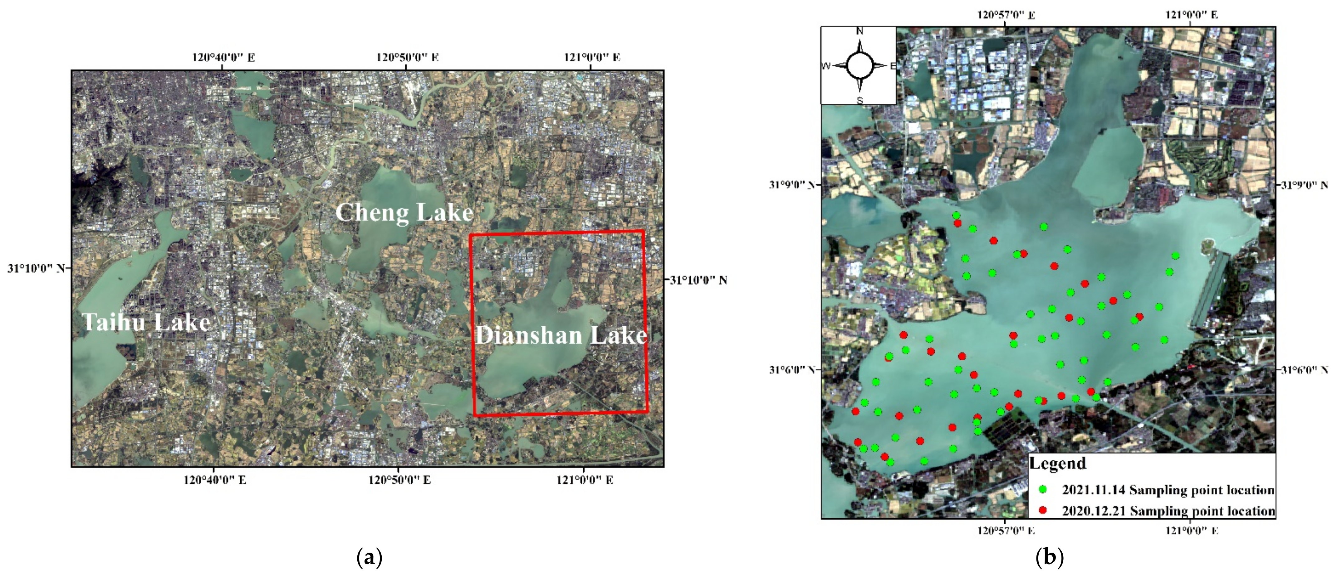
2.1. Study Area

Dianshan Lake (31°04′–31°12′ N, 120°54′–121°01′ E) is located in the lower reaches of the Yangtze River, at the junction of Shanghai and Jiangsu (see Figure 1). This lake is the largest natural lake in Shanghai, with a total area of approximately 62 km², of which 46.7 km (accounting for 75.3% of the entire lake) is in the Shanghai area. Dianshan Lake is a shallow lake in a plain water network area, and is shaped similarly to a gourd, that is, wide in the south and narrow in the north and its terrain is sloped from west to east. The lake mainly undertakes the inflow of water from the Taihu Lake Basin. The water flows through the Huangpu River to the mouth of the Yangtze River and into the East China Sea [26,27]. Many rivers go in and out of the lake, resulting in abundant water resources, giving the lake both economic and social significance.

2.2. Measured Data

Water samples were collected from Dianshan Lake on 21 December 2020 and 14 November 2021. The sky was cloudless, and the water surface was calm on the day of sampling. A total of 80 sampling points were used (see Figure 1). The geographic location information of sampling points was accurately recorded through global data corresponding to the sampling points. According to the principle of equilibrium and randomness, 80% of the sampling points were taken as the modeling points for the retrieval model, while the remaining 20% were used to test the retrieval performance of the model; that is, 64 sampling points were used for model construction and 16 sampling points were used for testing (location and Chl-a concentration of the test samples are listed in

Table 1. Location and Chl-a concentration of the test samples.

Sampling Point ID	Longitude (°)	Latitude (°)	Chl-a (μg/L)
ID1	120.9733	31.09405	4.11
ID5	120.9301	31.1049	2.00
ID9	120.9104	31.08038	1.42
ID16	120.9863	31.11427	1.47
ID21	120.947	31.13484	2.27
ID25	120.9523	31.10922	5.47
ID34	120.9283	31.07528	8.63
ID39	120.9294	31.09667	10.54
ID40	120.9364	31.09333	10.95
ID46	120.9297	31.10833	12.65
ID47	120.9472	31.09389	11.70
ID56	120.9778	31.09667	13.08
ID58	120.9636	31.10917	9.80
ID75	120.9669	31.1325	10.95
ID76	120.9761	31.125	13.07
ID77	120.9831	31.12028	10.95

). The Chl-a concentration of the samples was measured at the Shanghai University Engineering Research Center for Water Environment Ecology through acetone extraction spectrophotometry (statistical data of measured Chl-a concentration are shown in

Table 2. Statistical data of measured Chl-a concentration.

Date	Maximum Value (μg/L)	Minimum Value (μg/L)	Average Value (μg/L)
21 December 2020	6.84	0.95	3.15
14 November 2021	16.56	7.66	10.91
All	16.56	0.95	8.29

). The experimental principle involved extracting and determining the Chl-a concentration with the 90% acetone solvent through repeated grinding, extraction, and centrifugation. The acetone extraction spectrophotometric method is simple to operate and has high determination accuracy [28].

2.3. Landsat-8 Remote Sensing Image

The Landsat-8 data used in this research were obtained from the official website of the United States Geological Survey. The satellite parameters are shown in

Table 3. Parameters of Operational Land Imager sensor.

Band Name	Band Range (μm)	Spatial Resolution (m)
Band1 Coastal	0.433–0.453	30
Band2 Blue	0.450–0.515	30
Band3 Green	0.525–0.600	30
Band4 Red	0.630–0.680	30
Band5 NIR	0.845–0.885	30
Band6 SWIR1	1.560–1.660	30
Band7 SWIR2	2.100–2.300	30
Band8 PAN	0.500–0.680	15
Band9 Cirrus	1.360–1.390	30

. According to the principle of simultaneous registration, the Landsat-8 data covering the Dianshan Lake area on 22 December 2020 and 14 November 2021 were selected as the research objects. The cloud content of the 22 December 2020 image data was 0.61%, while that of the 14 November 2021 image data was 0.2%.

The data were captured by the Operational Land Imager sensor, and the radiance value (Digital Number value) was recorded. The Digital Number values in the remote sensing images needed to be converted into radiance values. Moreover, the sensor is affected by atmospheric molecules, cloud particles, aerosols, and other factors when receiving the reflection information of ground objects, resulting in atmospheric radiation information being present in the data. This leads to the spectral information of the ground objects differing from the obtained spectral information. Therefore, radiometric calibration and atmospheric correction of the images were required in order to ensure that accurate ground reflection information was obtained and, in turn, to ensure the accuracy of water quality monitoring through remote sensing data. After image preprocessing, the water body of Dianshan Lake was extracted, using a mask, for the subsequent band operations.

3. Research Methods

3.1. BP Neural Network Modeling Analysis

A huge sample size is generally required for BP neural network learning. Considering the time limitations associated to synchronous water sample collection, the sampling in the two phases was combined. The feasibility analysis was performed as follows:

(1)

The input parameter of the BP neural network was the water body reflectivity band combination. The water body reflectivity is related to the nature of the water body. As remote sensing data with the same pre-processing (radiometric calibration, atmospheric correction) were used, and as the image data used were all obtained in winter in the same study area, the homogeneity of the obtained water reflectance remote sensing images was ensured;

(2)

The water sample collection method and water Chl-a concentration measurement method were kept consistent for both times, ensuring the reliability and consistency of the accuracy of measured Chl-a concentration accuracy;

(3)

The results were derived according to the radiation transfer model formula given in [15]. The bottom reflectance can be ignored, as light cannot reach the bottom of the lake, due to its depth and transparency. Therefore, the main factors affecting the reflectance of the entire water body were the concentration of Chl-a and suspended solids.

In summary, adoption of the BP neural network model, the water reflectivity training samples, and the measured Chl-a concentrations were considered sufficient to establish a BP neural network prediction and retrieval model for chlorophyll concentration. Another influencing factor was the concentration of suspended solids. If measured data are available, then a predictive retrieval model can also be established.

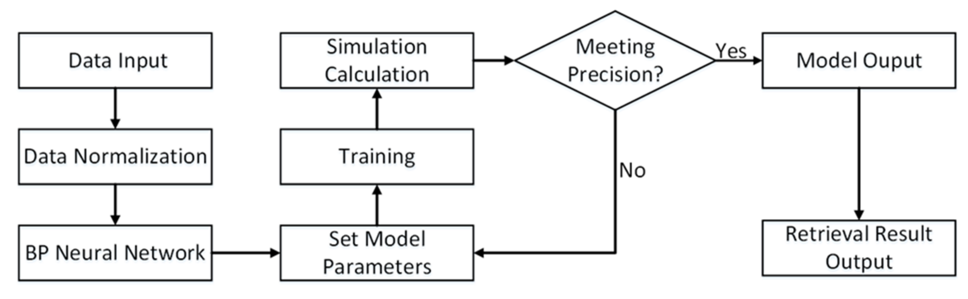
3.2. Principle of BP Neural Network Method

A BP neural network is a multi-layer feed-forward neural network trained using the error back propagation algorithm, which includes the forward and error backpropagation processes [29]. In the forward propagation process, the input is passed from the input layer to the hidden layer, processed layer-by-layer in the hidden layers, and then passed to the output layers. If an error exists between the output result and the expected value, then the error back propagation process is immediately executed. Next, a new round of forward propagation is performed after the backpropagation. The forward propagation and error back propagation processes are repeated until the minimum error between the expected value and the output result meets the requirements. The complete BP neural network structure mainly includes an input layer, several hidden layers, and an output layer, where each layer consists of several nodes (or neurons). The neurons in the same layer are not connected with or affected by each other. The state of each layer of neurons only has an impact on the state of the next layer of neurons, and all of the layers are connected. A three-layer shallow neural network with one hidden layer was used in this research [30]. The network has been shown to be capable of approximating any nonlinear function and learning and simulating complex nonlinear relationships [31].

3.3. Parameter Selection of BP Neural Network Model

The correlation between the measured Chl-a concentration data and corresponding single-band remote sensing reflectance was analyzed.

Table 4. Single-band correlation analysis.

Band	Correlation
Band1	−0.59
Band2	−0.36
Band3	−0.12
Band4	−0.10
Band5	−0.01
Band6	−0.16
Band7	−0.46

shows that some single bands were not highly correlated with the chlorophyll concentration. If the single band is directly used as an input to the BP neural network, then the validity of the Chl-a concentration retrieval cannot be guaranteed. Therefore, the correlation between the various bands of Landsat-8 and combinations of bands with the concentration of Chl-a requires further study.

A total of 436 combinations of bands were obtained in this research, where the highest correlation between the band combinations and the measured Chl-a concentration was 0.8, indicating a strong correlation, however, not all of the band combinations were highly correlated with the measured values. Therefore, according to the correlation, 66 combinations with a correlation higher than 0.5 or lower than −0.5 were selected, as listed in

Table 5. Band combination table by significance test.

Combination Methods	Correlation Coefficient	Combination Methods	Correlation Coefficient	Combination Methods	Correlation Coefficient
B1 + B7	−0.60	IN(B3/B2)	0.56	B3/B1/(B1 + B7)	0.79
B1 − B2	−0.71	IN(B3/B1)	0.69	B3/B1/(B1 − B7)	0.78
B1 − B3	−0.53	IN(B4/B1)	0.54	(B1 − B3)/(B7 − B1)	0.71
B1 − B7	−0.58	IN(B1)/IN(B7)	0.56	(B1 − B3)/(B1 − B7)	−0.71
B2 − B1	0.71	IN(B2)/IN(B1)	−0.51	(B1 − B3)/(B1 + B7)	−0.70
B3 − B1	0.53	IN(B1)/(B1 + B7)	−0.57	(B2 − B1)/(B7 − B1)	−0.66
B7 − B1	0.58	IN(B1)/(B1 − B7)	−0.56	(B2 − B1)/(B1 − B7)	0.66
B1 × B7	−0.63	IN(B1)/(B7 − B1)	0.56	(B2 − B1)/(B1 + B7)	0.67
B1/B4	−0.53	IN(B3/B1/(B1 + B7))	0.79	(B3 − B1)/(B7 − B1)	−0.71
B1/B3	−0.66	IN(B3/B1/(B1 − B7))	0.77	(B3 − B1)/(B1 − B7)	0.71
B1/B2	−0.66	B3/B1/(B7 − B1)	−0.78	(B3 − B1)/(B1 + B7)	0.70
B2/B3	−0.50	(B1 + B7)/B3/B1	−0.78	(B1 − B2)/(B7 − B1)	0.66
B2/B1	0.67	(B1 − B2)/B3/B1	−0.71	(B1 − B2)/(B1 − B7)	−0.66
B3/B2	0.60	(B1 − B7)/B3/B1	−0.76	(B1 − B2)/(B1 + B7)	−0.67
B3/B1	0.71	(B1 − B7)/B3/B1	0.71	(B1 + B7) + (B1 − B2)	−0.73
IN(B1)	−0.59	(B7 − B1)/B3/B1	0.76	(B1 + B7) + (B1 − B3)	−0.80
IN(B1−B7)	−0.57	(B1 + B7) − B3/B1	−0.80	(B1 + B7) + (B1 − B7)	−0.59
IN(B1/B4)	−0.54	(B1 − B2) − B3/B1	−0.72	(B1 − B2) + (B1 − B3)	−0.61
IN(B1/B3)	−0.69	(B1 − B3) − B3/B1	−0.65	(B1 − B3) + (B1 − B7)	−0.79
IN(B1/B2)	−0.66	(B1 − B7) − B3/B1	−0.80	(B2 − B1) + (B3 − B1)	0.61
IN(B2/B3)	−0.56	(B2 − B1) − B3/B1	−0.66	(B2 − B1) + (B7 − B1)	0.72
IN(B2/B1)	0.66	(B3 − B1) − B3/B1	−0.80	(B3 − B1) + (B7 − B1)	0.79

“IN” stands for exponential operation.

.

Among the 66 kinds of band combinations, the 3 band combinations with the highest correlation in the same combination type were selected, and the combination types without three items were eliminated. Nine band combination types remained, which are listed in

Table 6. List of used inputs.

Combination Methods	Combination Methods	Combination Methods
B1/B3	B2/B1	B3/B1
B1 − B2	B1 − B7	B2 − B1
IN(B1/B2)	IN(B1/B3)	IN(B3/B1)
IN(B1)/(B1 + B7)	IN(B1)/(B1 − B7)	IN(B1)/(B7 − B1)
(B1 + B7)/B3/B1	(B1 − B7)/B3/B1	(B7 − B1)/B3/B1
B3/B1/(B1+B7)	B3/B1/(B1 − B7)	B3/B1/(B7 − B1)
(B1 + B7) − B3/B1	(B1 − B7) − B3/B1	(B3 − B1) − B3/B1
(B1 − B3)/(B1 − B7)	(B3 − B1)/(B7 − B1)	(B3 − B1)/(B1 − B7)
(B1 + B7) + (B1 − B3)	(B1 − B3) + (B1 − B7)	(B3 − B1) + (B7 − B1)

.

Each of the nine combination types with high correlation in Table 6 were taken as an input to the input layer of the BP neural network. Meanwhile, the number of neuron nodes was determined using an empirical formula in order to prevent the model from suffering from overfitting due to excessive nodes or from the disconnection of the input and the output due to insufficient nodes [32]. The following empirical formula was used [33]:

$$Q=\sqrt{m+n+\alpha }$$

(1)

where Q is the number of hidden layer nodes, m is the number of input layer nodes, n is the number of output layer nodes, and α is in the range 0–10. Through calculation, the value range of the number of hidden layer nodes Q was 2–12.

3.4. Construction of BP Neural Network Model

As the input and output of the proposed BP neural network model were remote sensing reflectance values and Chl-a concentration, respectively, the range of variables should be unified and normalized before the network is established, within the range [−1, 1]. Before outputting the retrieval results, inverse normalization was required to output the real retrieval results. Then, the nine types of band combinations mentioned above were separately used as the input layer of the BP neural network model, with the retrieval Chl-a concentration as the output layer. The number of hidden layer nodes was 2–12, and the network training function adopted was trainlm. The activation function of the hidden layer was the sigmoid hyperbolic tangent function (tansig), and the output layer function used was the linear function (purelin). The maximum training times were set to 2000 times, and the convergence error was 0.00001 [34].

Through the repeated training and multiple tests of the model, the differences between the mean absolute error (MAE) and the coefficient of determination (R-squared) between the retrieval results with varying numbers of nodes in different hidden layers under the input layer of different combinations of the test samples and the corresponding measured Chl-a concentration from sampling were calculated. The best BP neural network model was determined by taking the mean absolute error and R-squared as the standard. The flow chart of building the BP neural network model is shown in Figure 2. Generally, the larger the R-squared and the smaller the mean absolute error, the higher the accuracy of the model and the smaller the deviation.

$$R^2=\frac{{\displaystyle {\sum }_{i=1}^n{(A_i-\overline{C})}^2}}{{\displaystyle {\sum }_{i=1}^n{(C_i-\overline{C})}^2}}$$

(2)

$$MAE=\frac{1}{n}{\displaystyle \sum _{i=1}^n\left|A_i-C_i\right|}$$

(3)

where C is the measured value, n is the number of samples (denoted by $i$ = 1, 2,⋯, n), $\overline{C}$ is the average of the measured values, and A is the value calculated by the retrieval model.

The R-squared, the root means square error (RMSE), and the mean relative error (MRE) were selected to serve as the standard of model accuracy evaluation. In general, the larger the R-Squared, the smaller the root mean square error, and the closer the mean relative error to 0, the higher the accuracy of the model and the smaller the bias.

$$RMSE=\sqrt{\frac{{\displaystyle \sum {}_{i=1}^n{\left(A_i-C_i\right)}^2}}{n}}$$

(4)

$$MRE=\frac{100\%}{n}{\displaystyle \sum _{i=1}^n\left|\frac{C_i-A_i}{C_i}\right|}$$

(5)

where C is the measured value, n is the number of samples, denoted by $i$ = 1, 2…, n, $\overline{C}$ is the average of the measured values, and A is the value calculated by the retrieval model.

3.5. Construction of Band Combination Model

Multiple linear regression and curve estimation analyses were used to construct a band combination retrieval model. Multiple linear regression analysis was used to select the top five band combinations as independent variables—namely, (B1 + B7) − B3/B1, (B1 − B7) − B3/B1, (B3 − B1) − B3/B1, (B1 + B7) + (B1 − B3), (B1 − B3) + (B1 − B7)), and the measured Chl-a concentration was the dependent variable. The multiple regression analysis was carried out using the SPSS software, and a retrieval model was constructed. The results are shown in

Table 7. Variables entered or removed.

Model	Input Variable	Removed Variable	Method
1	(B1 − B3) + (B1 − B7), (B3 − B1) − B3/B1, (B1 + B7) + (B1 − B3) b	(B1 + B7) − B3/B1, (B1 − B7) − B3/B1	Enter

^b “Tolerance = 0.000” limit reached.

,

Table 8. Model Fitting Results.

Model	R	R-Squared	Adjusted R-Squared	Error in Standard Estimation
1	0.782 a	0.611	0.591	2.629596385113078

^a Predictors: (constant), (B1 − B3) + (B1 − B7), (B3 − B1) − B3/B1, (B1 + B7) + (B1 − B3).

and

Table 9. Regression coefficient table.

Model		Unstandardized Coefficients		Standardized Coefficient		t	Salience
		B	Standard Error		Beta
1	Constant	−12.949	44.674			−0.290	0.773
	(B3 − B1) − B3/B1	−29.212	33.787		−0.397	−0.865	0.391
	(B1 + B7) + (B1 − B3)	−71.715	46.722		−2.218	−1.535	0.130
	(B1 − B3) + (B1 − B7)	61.410	46.942		1.840	1.308	0.196

below, where Table 7 shows the variables entered or removed, Table 8 provides the fitting results for the model, and Table 9 lists the coefficients of various variables in the model equation.

In summary, the following model equation was derived:

Chl-a = 61.41 × ((B1 − B3) + (B1 − B7)) − 29.21 × ((B3 − B1) − B3/B1) − 71.715 × ((B1 + B7) + (B1 − B3)) − 12.949

(6)

where Chl-a represents the retrieval result, B1 represents the remote sensing reflectance of Landsat-8 remote sensing data Band1, B3 represents the remote sensing reflectance of Landsat-8 remote sensing data Band3, and B7 represents the remote sensing reflectance of Landsat-8 remote sensing data Band7.

According to the above correlation analysis, the band combination with the highest correlation—namely, (B1 + B7) − B3/B1—was selected to conduct curve estimation analysis through the SPSS software, in order to construct a retrieval model. A total of four function retrieval models were constructed: namely, a linear function model, a quadratic function model, a cubic function model, and an exponential function model. As shown in

Table 10. Band combination model (curve estimation analysis).

Independent Variable	Model	Fitting Equation	R−Squared
(B1 + B7) − B3/B1	Linear function	Chl-a = − 17.445x − 1.9969	0.60
	Quadratic function	Chl-a = 12.581x2 − 3.9426x + 1.1729	0.61
	Cubic function	Chl-a = 141.29x3 + 232.44x2 + 101.5x + 16.359	0.65
	Exponential function	Chl-a = 1.0733e−3.121x	0.58

In the fitting equation, Chl-a represents the retrieval result, x is the independent variable (B1 + B7) − B3/B1,B1, B3 and B7 represent the remote sensing reflectivity of Landsat−8 remote sensing data Band1, Band3 and Band7.

below, the best fitting effect of the four function models was obtained with the cubic function model, and the fitting coefficient R² was 0.65.

4. Results

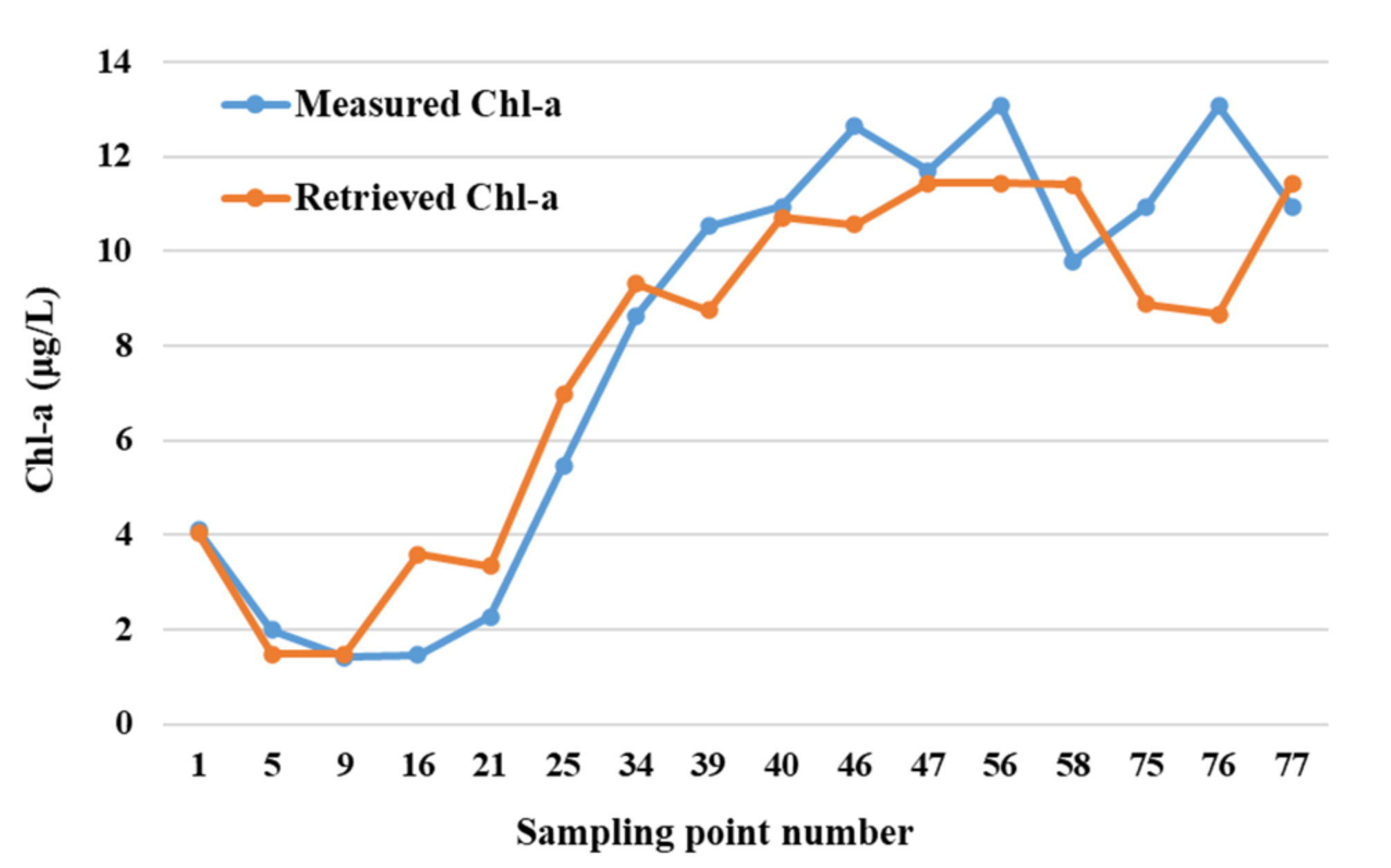
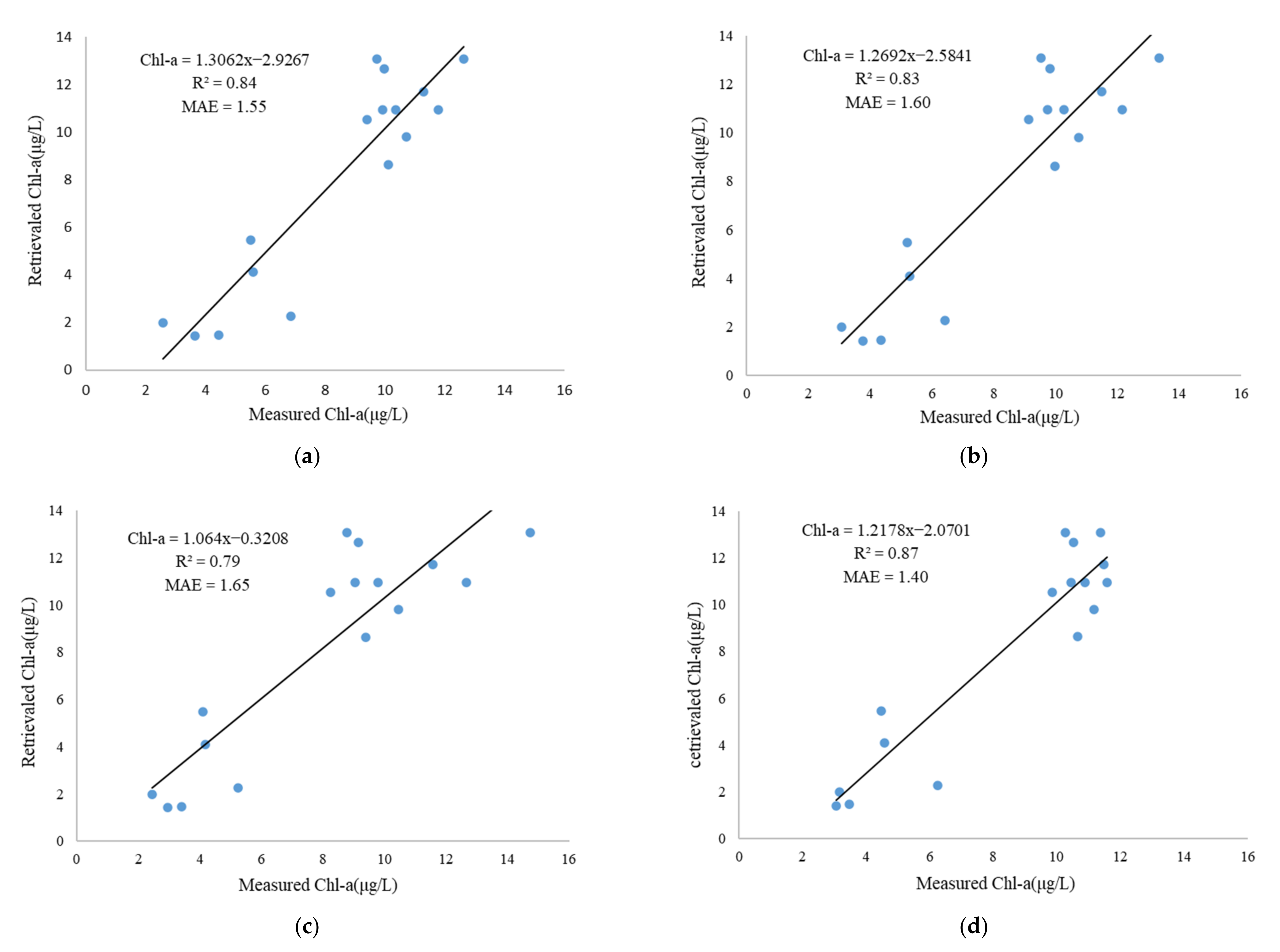
4.1. Results of the BP Neural Network Model

The results indicated that when the input layer of the BP neural network was set to the (B1 − B3)/(B1 − B7), (B3 − B1)/(B7 − B1), and (B3 − B1)/(B1 − B7) band combination and the number of neurons in the hidden layer was 2, the retrieval result of the BP neural network model presented the highest correlation with the measured value, with an R-Squared value of 0.86, and a mean absolute error of 1.28.

This optimal BP neural network model was used to retrieve the Chl-a concentration for the test sample. The retrieval results and the corresponding measured Chl-a concentration were analyzed for precision evaluation. The results demonstrated that the R-Squared value of the retrieval results between the test samples and the measured values was 0.86, the root mean square error was 1.69 μg/L, and the average relative error was 19.48%. Figure 3 clearly shows that the measured values showed the same trend as the retrieval result, indicating the small retrieval error of the model and its good retrieval effect.

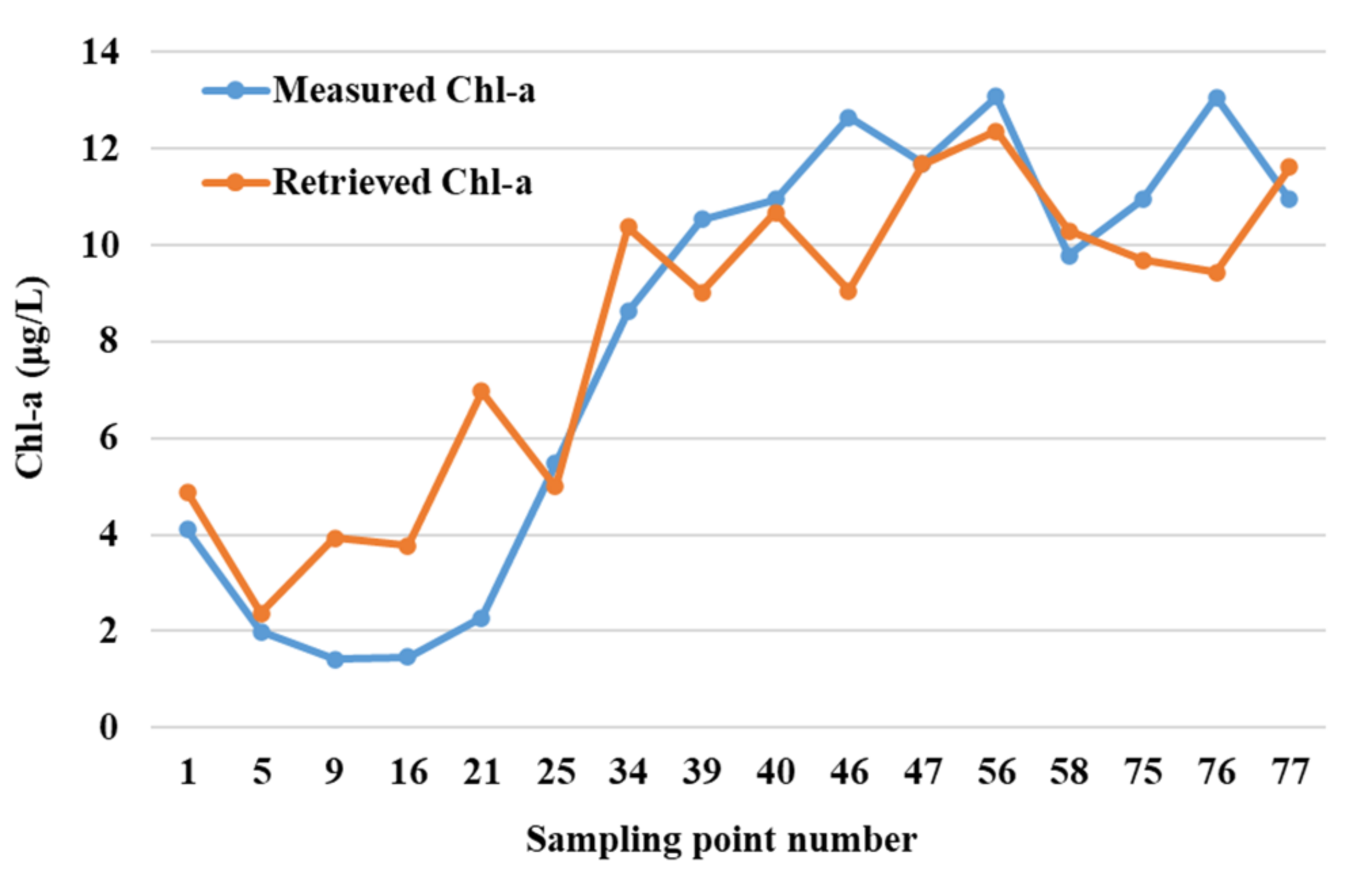
4.2. Results of the Band Combination Model

Chl-a concentrations were retrieved using the model constructed by multiple regression analysis. The results indicate that the R-Squared value of the retrieval results of the test samples and the measured values was 0.8, the root mean square error was 2.08 μg/L, and the average relative error was 23.62%. A comparison between the retrieval results and the measured values are shown in Figure 4. The retrieval results of the model constructed by multiple regression analysis and the measured values showed the same trend of change, and the error was relatively small. When the chlorophyll concentration was low, the concentration value was overestimated.

The four functional models constructed by curve estimation analysis were used to carry out retrieval for comparison. The mean absolute error and R-Squared of the retrieval results and the measured values were used as criteria to determine the best retrieval model. It can be seen from Figure 5 that the coefficient of determination of the cubic function model was the highest, and the mean absolute error was the smallest. Among the four models, the best fitting effect was achieved by the cubic function model (see Table 10). Therefore, the cubic function model was determined to be the best retrieval model among the four models constructed by curve estimation analysis and, so, the cubic function model was used for retrieval.

A comparison between the retrieval results of the cubic function model and the measured values is shown in Figure 6. The retrieval results of the cubic function model and the measured values showed a similar trend, and the error was smaller than that of the model constructed by multiple regression analysis. However, the same situation of overestimating the concentration values was observed: when the chlorophyll concentration was low, the concentration value was overestimated.

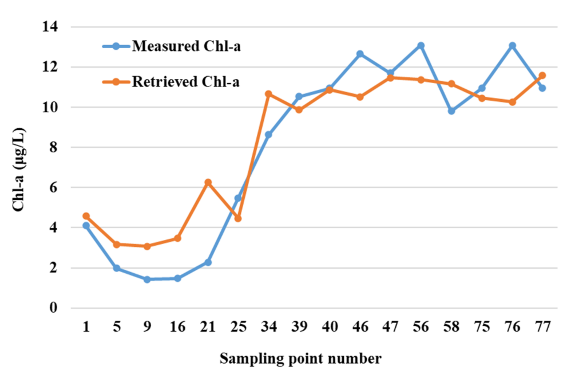
4.3. Comparative Analysis of Model Results

Accuracy evaluation and an analysis of the retrieval models were carried out, and the retrieval effects of the models were compared; the results are shown in

Table 11. Comparison of the accuracy evaluation results for the three models.

Index	Band Combination Model—Multiple Regression Analysis	Band Combination Model—Curve Estimation Analysis	BP Neural Network Model
R-Squared	0.80	0.87	0.86
RMSE (μg/L)	2.08	1.72	1.69
MRE (%)	23.62	22.45	19.48

below. The retrieval effect of the model constructed using curve estimation analysis was better than that of the model constructed by multiple regression analysis, showing a higher R-Squared value. The mean relative error and the root mean square error were also smaller than those of the multiple regression analysis-based model. Therefore, among the models constructed by the two regression methods, the model constructed by curve estimation analysis was more suitable for the Dianshan Lake research area. Among the three retrieval models, the BP neural network model presented the smallest the mean relative error and root mean square error, with mean relative error lower than 20% and R-Squared value of 0.86. Therefore, the proposed model has certain feasibility. In general, the retrieval accuracy of the BP neural network model was better than that of the band combination model. However, the correlation between the model retrieval results and the measured values was slightly worse than that of the retrieval model constructed by curve estimation analysis.

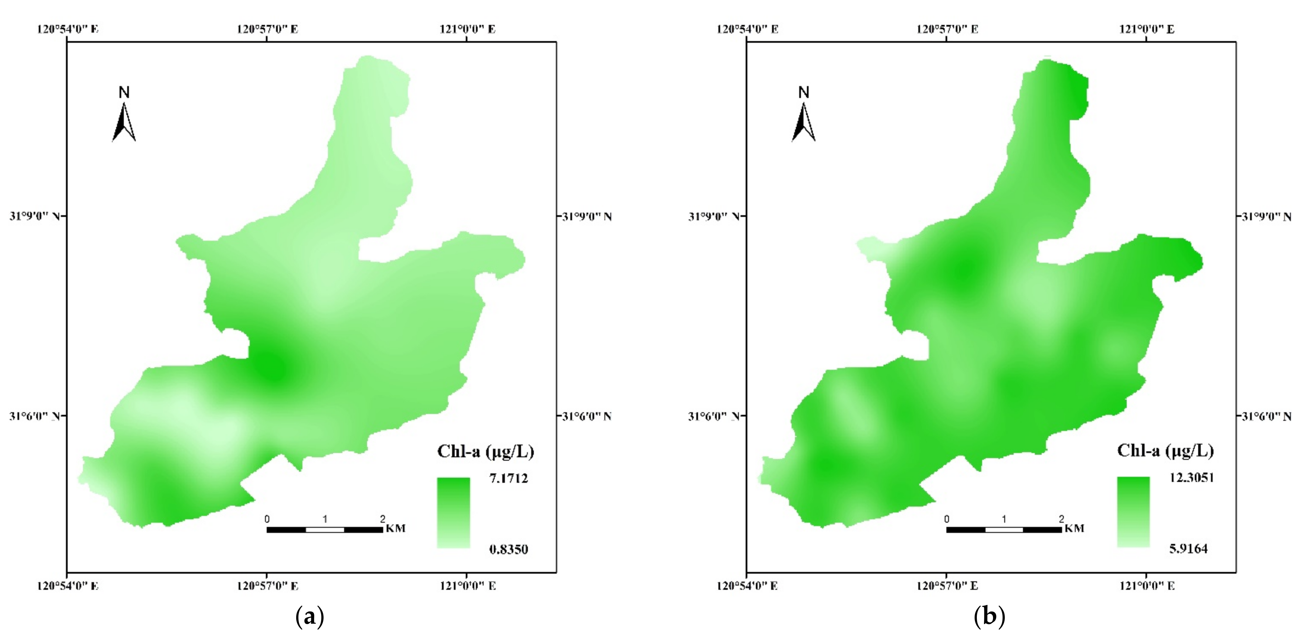
4.4. Spatiotemporal Analysis of Chl-a Concentration

In this research, preprocessed Landsat-8 remote sensing data were used for band operations. Combined with the optimal BP neural network model selected above, where the input to the BP neural network was (B1 − B3)/(B1 − B7), (B3 − B1)/(B7 − B1), (B3 − B1)/(B1 − B7); the number of nodes in the hidden layer was 2; and the number of nodes in the output layer was 1—Chl-a concentration in the water body of Dianshan Lake for 2020 and 2021 was retrieved. According to the spatial distribution of the retrieval results, as shown in Figure 7, the concentration of Chl-a in Dianshan Lake in 2021 was nearly double that in 2020: the concentration of Chl-a in 2020 was in the range of 0.84–7.17 μg/L, while that in 2021 is in the range of 5.91–12.31 μg/L. From the perspective of spatial distribution, the Chl-a concentration in Dianshan Lake was unevenly distributed and, so, the concentration of Chl-a in the lake varied greatly. This was mainly because Dianshan Lake receives incoming water from Taihu Lake, with many rivers entering and exiting, such that the water body in the lake has strong fluidity. It is also affected by human production and living, as well as the sewage discharge from aquaculture areas, making the Chl-a concentration near the shore higher than that in the open center of the lake.

5. Discussion

In the paper, two types of band combination models and a BP neural network model were constructed. In order to construct two types of band combination models, firstly we combined the bands of remote sensing images by using four operations of mathematics and logarithmic operations. These operations could improve the correlation between remote sensing reflectivity and Chl-a concentration in water, as well as the retrieval effect of Chl-a concentration in water. Then multiple linear regression analysis and curve estimation analysis were used, respectively, as algorithms for constructing two types of band combination models.

Comparison to other papers [1,9,11,15,18], two types of regression analyses to construct the band combination model. Furthermore, we discovered that the band combination model based on curve estimation analysis had a better retrieval effect, R-Squared is 0.87, root mean square error is 1.72 μg/L, and average relative error is 22.45%. When the retrieval effect of the band combination model of literature 11 and literature 15 [11,15] was examined, the R-Squared of both was less than 0.87. Compared with the retrieval accuracy of the literature 11 and 15 band combination models, the retrieval accuracy of this paper has been improved. This may be because the modeling method in this paper found the best band combination of correlation and the most appropriate regression analysis method to build the band combination retrieval model.

Studies have shown that [11,21,24,25,33] the BP neural network model has a better retrieval effect than the retrieval model based on empirical and semi-empirical methods, and its R-Squared higher than 0.8 and root mean square error within a reasonable range. The results of this research also revealed that the BP neural network model retrieval impact was better than the band combination model, with an R-Squared of 0.86 and a root mean square error of 1.69 μg/L mean relative error of 19.48%. This demonstrates that the BP neural network is adaptable in retrieving Chl-a concentrations in aquatic bodies.

The BP neural network model was compared to various neural network models, such as the convolutional neural network model and the hybrid neural network model [22,23]. The BP neural network model was relatively easy to construct, had a rapid processing rate, and can mimic nonlinear connections in complicated water bodies [31]. Although the convolutional neural networks model had the characteristics of minimizing noise sensitive and learning high abstraction and was suited for recovering Chl-a concentration in the Pearl River estuary, which includes turbid water bodies [22], its model construction is difficult. Furthermore, Dianshan Lake is an inland lake, and the water body’s features differ from those of the Pearl River estuary, especially pollutant and suspended matter concentrations. The research has also shown simplicity and better accuracy, using the BP neural network model to retrieval Chl-a concentration of Dianshan Lake water body in the paper.

However, when compared to other studies on the retrieval of Chl-a concentration in water bodies [1,22,32,33], the number of samplings in our study was low. Therefore, the number of samplings should be increased in order to achieve long series quantitative retrieval of Chl-a concentration in Dianshan Lake water bodies.

As the same sensor data were used for the two phases and the remote sensing image data underwent the same preprocessing (i.e., radiometric calibration, atmospheric correction, and water and land separation), the nature and quality of data used as the input to neural network were ensured to be uniform. The experimental results presented in this paper indicate that the joint retrieval of data considering two phases is feasible. The different altitude and azimuth angles of the satellite and the sun when the two phases of remote sensing data are imaged may influence the retrieval results; this effect will be investigated in the future.

6. Conclusions

Based on two phases of Landsat-8 satellite images and measured the Chl-a concentration data, we constructed two types of band combination model and a BP neural network model to retrieve the Chl-a concentration in Dianshan Lake. The band combination models were constructed by using multiple linear regression analysis and curve estimation approaches in order to identify the modeling approach better adapted to the study area and obtain optimal retrieval results. The results demonstrated that the accuracy of the best curve estimation analysis-based model was higher than that of the multiple regression analysis-based model, making the former more applicable for the retrieval of the Chl-a concentration in Dianshan Lake.

Comparative analysis of the retrieval results from the combination models and the BP neural network model indicate that the BP neural network model has certain advantages; namely, the BP neural network model obtained the highest retrieval accuracy and the best retrieval effect, and the BP neural network model successfully retrieved the Chl-a concentration in Dianshan Lake. Therefore, the proposed model can provide research guidance for the subsequent retrieval of Chl-a concentration in Dianshan Lake and has certain reference for the retrieval of Chl-a concentration in other third-class water bodies. Thus, it has certain practical significance. Moreover, joint retrieval in two phases can allow us to overcome the shortcomings associated with a lack of measured data and provides new ideas for water quality monitoring over a large area.

References

1. Song, T.; Zhou, W.; Liu, J.; Gong, S.; Shi, J.; Wu, W. Evaluation on distribution of chlorophyll-a content in surface water of Taihu Lake by hyperspectral inversion models. Acta Sci. Circumstantiae 2017, 37, 888–899. [Google Scholar]
2. Cheng, C.; Li, Y.; Ding, Y.; Tu, Q.; Qin, P. Remote Sensing Estimation of Chlorophyll-a and Total Suspended Matter Concentration in Qiantang River Based on GF-1/WFV Data. J. Yangtze River Sci. Res. Inst. 2019, 36, 21–28. [Google Scholar]
3. Honeywill, C.; Paterson, D.M.; Hegerthey, S.E. Determination of microphytobenthic biomass using pulse-amplitude modulated minimum fluorescence. Eur. J. Phycol. 2002, 37, 485–492. [Google Scholar] [CrossRef]
4. Zhu, G.; Xu, H.; Zhu, M.; Zou, W.; Guo, C.; Ji, P.; Da, W.; Zhou, Y.; Zhang, Y.; Qin, B. Changing characteristics and driving factors of trophic state of lakes in the middle and lower reaches of Yangtze River in the past 30 year. J. Lake Sci. 2019, 31, 1510–1524. [Google Scholar]
5. Kang, L. Study on Eutrophication Process and Water Ecological Effect of Dianshan Lake. Environ. Sci. Manag. 2020, 45, 171–174. [Google Scholar]
6. Behmel, S.; Damour, M.; Ludwig, R.; Rodriguez, M.J. Water quality monitoring strategies—A review and future perspectives. Sci. Total Environ. 2016, 517, 1312–1329. [Google Scholar] [CrossRef] [PubMed]
7. Le, C.; Li, Y.; Sun, D.; Wang, H.; Huang, C. Spatio-temporal Distribution of Chl-a Concentration, and Its Estimation in Taihu Lake. Environ. Sci. 2008, 29, 619–626. [Google Scholar]
8. Tian, Y.; Guo, Z.; Qiao, Y.; Lei, X.; Xie, F. Remote sensing of water quality monitoring in Guanting Reservoir. Acta Ecol. Sin. 2015, 35, 2217–2226. [Google Scholar]
9. Li, J.; Pei, Y.; Zhao, S.; Xiao, R.; Sang, X.; Zhang, C. A review of remote sensing for environmental monitoring in China. Remote Sens. 2020, 12, 1130. [Google Scholar] [CrossRef] [Green Version]
10. Zhang, Y.; Zhang, Y.; Cha, Y.; Shi, K.; Zhou, Y.; Wang, M. Remote sensing estimation of total suspended matter concentration in Xin’anjiang reservoir using Landsat 8 data. Environ. Sci. 2015, 36, 56–63. [Google Scholar]
11. Dan, Y.; Zhou, Z.; Li, S.; Zhang, H.; Jiang, Y. Inversion of Chlorophyll-a Concentration in Pingzhai Reservoir Based on Sentinel-2. Environ. Eng. 2020, 38, 180–185. [Google Scholar]
12. Huang, Y.; Jiang, D.; Zhuang, D.; Fu, J. Research on remote sensing estimation of chlorophyll concentration in water body of Tangxun Lake. J. Nat. Disasters 2012, 21, 215–222. [Google Scholar]
13. Mu, B.; Cui, T.; Cao, W.; Qin, P.; Zheng, R.; Zhang, J. A Semi-analytical monitoring method during the process of red tide based on optical buoy. Acta Opt. Sin. 2012, 32, 8–16. [Google Scholar]
14. Li, Y.; Huang, J.; Wei, Y.; Lu, W. Inversing Chlorophyll concentration of Taihu Lake by ana lytic model. J. Remote Sens. 2006, 10, 169–175. [Google Scholar]
15. Yang, X.; Jiang, Y.; Deng, X.; Zheng, Y.; Yue, Z. Temporal and spatial variations of Chlorophyll a concentration and eutrophication assessment (1987–2018) of Donghu Lake in Wuhan using Landsat images. Water 2020, 12, 2192. [Google Scholar] [CrossRef]
16. Zhang, L.; Dai, X.; Bao, Y.; Wu, J.; Yu, C. Inversion of chlorophyll-a concentration based on TM images in Wuliangsuhai Lake. Environ. Eng. 2015, 33, 133–138. [Google Scholar]
17. Liu, W.; Deng, R.; Liang, Y.; Wu, Y.; Liu, Y. Retrieval of chlorophyll-a concentration in Chaohu based on radiative transfer model. Remote Sens. Land Resour. 2019, 31, 102–110. [Google Scholar]
18. Xie, T.; Chen, Y.; Lu, W. Retrieval of chlorophyll-a in the lower reaches of the Minjiang River via three-band bio-optical model. Lasers Optoelectron. Prog. 2020, 57, 1–8. [Google Scholar]
19. Pan, C.; Xia, L.; Wu, Z.; Wang, M.; Xie, X.; Wang, F. Remote sensing retrieval of chlorophyll-a concentration in coastal aquaculture areaof Zhelin Bay. J. Trop. Oceanogr. 2020, 40, 142–153. [Google Scholar]
20. Wu, Y.; Deng, R.; Qin, Y.; Liang, Y.; Xiong, L. The study of characteristics for Chlorophyll Concentration derived remote sensing in Xinfengjiang Reservoir. Remote Sens. Technol. Appl. 2017, 32, 825–834. [Google Scholar]
21. Zhang, Y.; Pulliainen, J.T.; Koponen, S.S.; Martti, T.H. Water quality retrievals from combined Landsat TM data and ERS-2 SAR data in the Gulf of Finland. IEEE Trans. Geosci. Remote Sens. 2003, 41, 622–629. [Google Scholar] [CrossRef]
22. Ye, H.; Tang, S.; Yang, C. Deep learning for Chlorophyll-a concentration retrieval: A case study for the Pearl River Estuary. Remote Sens. 2021, 13, 3717. [Google Scholar] [CrossRef]
23. Xue, L.; Jian, S.; Zhong, L. Chlorophyll-A Prediction of Lakes with Different Water Quality Patterns in China Based on Hybrid Neural Networks. Water 2017, 9, 524. [Google Scholar] [CrossRef] [Green Version]
24. Zhang, X.; Zheng, X. Discussion on retrieval method of surface Chlorophyll concentration in Bohai Bay based on BP neural network. J. Ocean Technol. 2018, 37, 79–87. [Google Scholar]
25. Zhu, Y.; Zhu, L.; Li, J.; Chen, Y.; Zhang, Y.; Hou, H.; Ju, X.; Zhang, Y. The study of inversion of Chl-a in Taihu based on GF-1 WFV image and BP neural network. Acta Sci. Circumstantiae 2017, 37, 130–137. [Google Scholar]
26. Zhang, Y.; Zhang, D.; Sun, Z. Water quality and water environmental assessment of Dianshan Lake in Shangha. J. Water Resour. Water Eng. 2017, 28, 90–96. [Google Scholar]
27. Wang, S.; Qian, X.; Zhao, G.; Zhang, W.; Zhao, Y.; Fan, Z. Contribution analysis of Pollution Sources Around Dianshan Lake. Resour. Environ. Yangtze Basin 2013, 22, 331–336. [Google Scholar]
28. Li, Z.; Lu, J.; Wang, G.; Ge, X. Comparison of measurement of phytoplankton Chlorophyll-a concentration by spectrophotometry. Environ. Monit. China 2006, 22, 21–23. [Google Scholar]
29. Ma, H.; Liu, S. The Potential Evaluation of Multisource Remote Sensing Data for Extracting Soil Moisture Based on the Method of BP Neural Network. Can. J. Remote Sens. 2016, 42, 117–124. [Google Scholar] [CrossRef]
30. Wang, S.J.; Guan, D.S. Remote Sensing Method of Forest Biomass Estimation by Artificial Neural Network Models. Ecol. Environ. 2007, 16, 108–111. [Google Scholar]
31. Hinton, G.E. Reducing the dimensionality of data with neural networks. Science 2006, 313, 504–507. [Google Scholar] [CrossRef] [PubMed] [Green Version]
32. Fan, Y.; Liu, J. Water depth remote sensing retrieval model based on Artificial Neural Network Techniques. Hydrogr. Surv. Charting 2015, 165, 20–23. [Google Scholar]
33. Xu, P.; Cheng, Q.; Jin, P. Inversion of Chlorophyll-a of clean water in Qiandao Lake With remote sensing data using the neural network. Resour. Environ. Yangtze Basin 2021, 30, 1670–1679. [Google Scholar]
34. Zhou, L.; Gu, X.; Zeng, Q.; Zhou, W.; Mao, Z.; Sun, M. Applications of Back Propagation Neural Network for Short-term Prediction of Chlorophyll-a Concentration in Different Regions of Lake Taihu. J. Hydroecol. 2012, 33, 1–6. [Google Scholar]
Figure 1. Geographical location of the study area and distribution of sampling points: (a) Study area location; and (b) sampling point locations.
Sustainability 14 08894 g001
Figure 2. BP neural network model modeling flow chart.
Sustainability 14 08894 g002
Figure 3. Retrieval results of BP neural network model and the measured values.
Sustainability 14 08894 g003
Figure 4. Retrieval results of multiple regression analysis-based model and measured values.
Sustainability 14 08894 g004
Figure 5. Four models constructed by curve estimation analysis: (a) Linear function model (b) quadratic function model (c) cubic function model; and (d) exponential function model.
Sustainability 14 08894 g005
Figure 6. Retrieval results of curve estimation analysis-based model and measured values.
Sustainability 14 08894 g006
Figure 7. Retrieval map of Chl-a in Dianshan Lake: (a) Chl-a retrieval concentration distribution map obtained for 22 December 2020; and (b) Chl-a retrieval concentration distribution map obtained for 14 November 2021.
Sustainability 14 08894 g007