Dynamic Rule Curves and Streamflow under Climate Change for Multipurpose Reservoir Operation Using Honey-Bee Mating Optimization

Abstract

Climate change in the watershed above the reservoir has a direct impact on the quantity of streamflow that enters the reservoir and the management of water resources. Developing effective reservoir rule curves helps reduce the risk of future failures of water resource management. The purpose of this study was to analyze the influence of climate change on the volume of streamflow entering the Ubolratana Reservoir, Thailand during the years 2020–2049 with climate simulations from the CIMP5 model under RCP4.5 and RCP8.5 scenarios. SWAT models were used to forecast future reservoir streamflow quantities. Moreover, suitable reservoir rule curves using the Honey-Bee Mating Optimization (HBMO) were developed and the effectiveness of the new rule curves was assessed. According to the research findings, the average yearly streamflow in the future apparently grew from 32% in the base years (2011–2019) and 65% under the RCP4.5 and RCP8.5 scenarios, respectively. It was discovered that the average monthly streamflow was higher in the rainy season than in the dry season. Both of the projected situations have a form compatible with the present rule curves in the section of the new reservoir rule curves generated with the HBMO. Furthermore, the newly constructed rule curves may allow the reservoir to keep more water during the rainy season, thereby assuring that there will be adequate water during the following dry season. Additionally, during the dry season, the reservoir was able to release more water that would be able to reduce the water shortage, indicating that it was able to effectively reduce the amount of water shortage and average overflow under RCP4.5 and RCP8.5 situations.

1. Introduction

Uncertainty has a direct influence on the understanding of hydrology and water resource cycles caused by global climate change, as well as the growing frequency and intensity of droughts and floods throughout the world; these events are jeopardizing the management and development of water resources to meet global demands in all industries, making management more complex and difficult. For the past two decades, climate change has had a global impact on water resource management. Several study groups have sought to create ways for controlling water at its sources in order to deal with the fluctuation of supply sides and demand sides. The majority of such studies have evaluated the consequences of future climate change based on prediction findings from climate models combined with hydrological models to analyze impacts on water allocation efficiency for consumption [1], irrigation [2,3] hydroelectric power generation [4], and procurement of new reservoirs in the future [5].

In Thailand after the Great Flood of 2011, numerous watershed areas experienced drought between 2012 and 2019. The primary reason for this is that rainfall was below normal [6]. Many rivers’ average discharge was lower than usual [7]. Government agencies must implement campaign initiatives to encourage consumers and farmers to consume water most efficiently and cost-effectively as possible. The northeastern area of Thailand comprises more than 60% agricultural land and is mostly dependent on seasonal rainfall in off-season cultivation, especially for rice cultivation, as it requires water from irrigation systems which rely on the cost of water from reservoirs. Meanwhile, the demand for water downstream in various sectors tends to increase. Many large and medium-sized reservoirs are unable to allocate water to meet the needs of all sectors effectively. In addition, the development of water resource management through efficient tools and methodology, alongside the consideration of the conditions of complex and nonlinear problems in all dimensions, is required especially for the management of reservoir water resources in situations of global climate change volatility [5]. It is, therefore, necessary to make an urgent adjustment.

Over the past decade, climate and streamflow were included in future hydrological models. These two factors have been used in combination with reservoir management. It is an approach that has been widely used in studies across the world. In Thailand, the Hydro-Informatics Institute created and released the Coupled Model Intercomparison Project Phase 5 (CMIP5) family of global climate models. This model has undergone bias correction using a Gamma-Gamma (GG) transformation optimization approach [8] to make future computation results more dependable. The products from CMIP5 have been used to analyze the effects of climate change in Thailand’s watershed areas [9], hydrological systems in Southeast Asia [10], and many other places across the world [11,12].

A hydrological model is used to forecast future streamflow. In this study, a semi-diffuse hydrological model was investigated. The SWAT [13] is the world’s most popularly used climate model, because of its integration of geographic information (GIS) data and regional climatic data in watershed areas of every size. As a result, the analysis is trustworthy. SWAT has been used in Thailand to examine and analyze the quantity of streamflow in various scenarios [14,15], and for the future management [16,17] of water resources in watersheds and reservoirs [18]. The precision of SWAT calculation results could improve when compared to the real measurements and this was accomplished by employing the SWAT-CUP model and the SUFI-2 approach [19] to choose the most appropriate sensitivity variables for analyzing the studied watershed regions. Therefore, based on the strengths of the CMIP5-derived products, once they were imported into SWAT, the results were expected to be future streamflow that differ from the new projection of greenhouse gas emissions. The Representative Concentration Pathway (RCP) as defined in the fifth Assessment Report (AR5) by the IPCC [20] provides cost information for appropriate reservoir management to situations of future hydrological variation.

There have already been some studies on applying optimization techniques to reservoir management, particularly in the development of suitable reservoir rule curves. Mathematicians have created evolutionary optimization approaches throughout the last decade. Appropriate reservoir rule curves were created using metaheuristic optimization techniques. Several approaches are popular in Thailand and across the world, such as Genetic Algorithm (GA) [18,21,22,23] Ant Colony Optimization (ACO) [24], Firefly Algorithm (FA) [25], Grey Wolf Optimization (GWO) [26], Tabu Search Algorithm (TSA) [27,28], and Particle Swarm Optimization (PSO) [21,22]. However, a new kind of evolutionary technique has been created, which is a natural-inspired approach to solving problems and finding answers in engineering. It is the Honey-Bee Mating Optimization (HBMO) algorithm [29], a process for optimization by imitating bee swarm behavior.

However, the solution to reservoir water allocation challenges caused by climate change affects future streamflow volumes. It was discovered that there were not many studies in the northeastern part of Thailand, along with forecasts of the variance in water demand from diverse activities in the downstream areas, especially for reservoirs in remote places where functionality is essential. Ubolratana Reservoir is the first significant multi-purpose reservoir in Thailand’s northeast that provides hydroelectric electricity by combining irrigation and rainwater harvesting to reduce floods during the wet season. However, in the last ten years, dry-season water resource management has encountered a water insufficiency problem. Water intake to reservoirs has been lower than the average amount. In contracts, in certain years, the volume of water flowing into the reservoir surpasses the storage capacity during the rainy season. The water must be drained onto the downstream side, causing floods in residential and agricultural regions. As a result, when Ubolratana Reservoir has to develop suitable and efficient water distribution criteria, taking into account the diversity of hydrological circumstances in the past, present, and future together with the application of evolutionary optimization techniques to create more efficient rule curves. This would be expected to be of great benefit for water resource management.

In the past, the consideration of improving the reservoir rule curves of Ubolratana Reservoir, and the other reservoirs in Northeastern Thailand was a case study based on climate change forecasting from the AR4 models [18,30]. This research draws on climate forecasting data from the CMIP5 model based on the RCP4.5 and RCP8.5 scenarios that use bias correction to be more accurate, including there are various types and different model resolutions. The integration of SWAT hydrological models into the analysis of streamflow conditions has not been previously studied, and the same applies to experiments that link these models to the development of the optimal reservoir rule curves with the HBMO technique. Consequently, the expected outcome of the study is the optimal rule curves, appropriate outcome for the climate change situation and the variation on streamflow in many cases.

The purpose of this research was to use the CMIP5 and SWAT models to examine how global climate change affects the quantity of streamflow input into the Ubolratana Reservoir, as well as to improve the reservoir rule curves by employing the approach of the HBMO and considering the objective function, which is to minimize the quantity of water that is scarce and the amount of water that overflows the reservoir, respectively. The results of this study were predicted to be useful in predicting water scarcity and extreme water circumstances for flexible water management, provided as decision-support information for stakeholders to use as information for climate change policy planning and evaluation of water allocation guidelines to assist future activities.

2. Materials and Methods

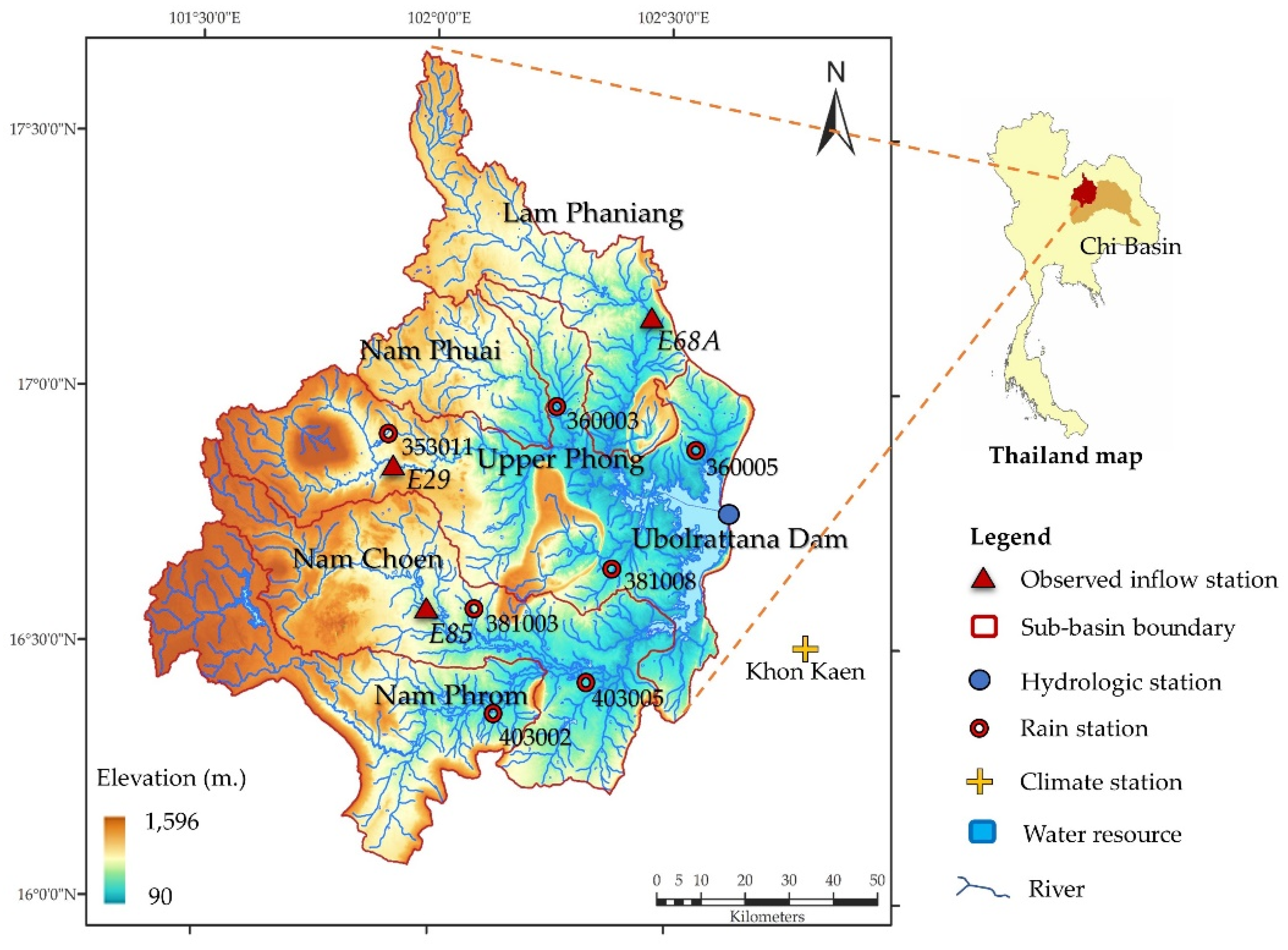
2.1. Research Area

The research site was Ubolratana Reservoir in Ubolratana District, Khon Kaen Province. The study focused on five watershed areas; Lam Pha Niang, Lam Nam Phue, Upper Lam Nam Phong, Lam Nam Choen, and Lam Nam Phrom, all of which are tributaries of the Chi River Basin in northeast Thailand (Figure 1), with a total water intake area of around 12,000 square kilometers. The reservoir is a rock-fill dam with a clay core with a height of 2 m. The dam crest is 185.00 m above sea level. The basin receives an average of 2470 MCM of water each year. The normal water storage capacity is 2431.3 MCM, with a reservoir area of 370 square kilometers. The main functions of the reservoir are for generating electricity with an annual power generation capacity of approximately 56.1 million kilowatt-hours, irrigation covering an area of approximately 480 square kilometers, flood relief, fisheries, and intercity transportation travel.

2.2. World Climate Models

2.2.1. CMIP5 Model

GCMs (General Circulation Models) are useful for describing and forecasting future climate change patterns. The World Meteorological Organization’s Global Climate Research Program is now collecting data on current global climate change under the acronym Coupled Model Intercomparison Project Phase 5 (CMIP5) [31]. For this study, 10 CMIP5 models were selected by the investigators: MIROC_ESM, BNU, CanESM, MIROC5, FGOALS_g2, CESM1_CAM5, GFDL, EC_EARTH, CCSM4, and FGOALS_s2 [32,33]. The data used in the global climate change analysis were supported by the Hydro-Informatics Institute (HII) (Public Organization), which revealed that there are a wide variety of models that can be applied (more than 15 models). However, when comparing the model’s data with the measurement stations in the study area, (especially rainfall data) and ranked based on the lowest tolerance. It was found that the models used in this study were among the 10 models with the lowest inaccuracies and were used in this study. Then, in the streamflow analysis, only the climate data from five of the best models were selected. For ease of use, the HII, which has downscaled the data model to a 5 × 5 square kilometer grid. Base year climate data in the study areas used the data for 9 years between 2011–2019, and climate forecasting data from 30-year models between 2020–2049.

2.2.2. Data Bias Correction

The Gamma-Gamma transformation approach was used in this study to correct for rainfall inaccuracy from the GCM. For this study, climate data, particularly precipitation data, courtesy of the Hydro-Informatics Institute (HII), is the agency that produces and distributes data for use in climate change studies in Thailand. This agency has identified the Gamma-Gamma transformation method to mitigate discrepancies in rainfall data. In addition, HII has published a study that applied this method to study the impact of climate change in Thailand on agricultural water demand [34]. In addition, Sharma (2015) has also chosen this method to study rainfall in western Thailand, which found that the Gamma-Gamma transformation was more effective in improving rainfall frequency and intensity compared to other methods [35]. The concept of this method is to correct for discrepancies caused by frequency and rainfall between GCM and measurement stations in the base year by creating a cumulative distribution function (CDF). This leads to the creation of appropriate Gamma parameters, with the functionalities and key parameters as shown in Equations (1)–(4).

$$F\left(x;\alpha ,\beta \right)=\frac{1}{{\beta }^{\alpha }\Gamma \left(\alpha \right)}{x}^{\alpha -1}\mathit{exp}\left(\frac{x}{\beta }\right);x\ge x_{Trunc}$$

(1)

$$F\left(x;\alpha ,\beta \right)={{\displaystyle \int }}_{x_{Trunc}}^{x}f\left(t\right)dt$$

(2)

$$F(x_{GCM};\alpha ,\beta |GCM)\Rightarrow F(x_{His};\alpha ,\beta |His)$$

(3)

$$x_{GCM}^{\prime }=F^{-1}\left\{F(x_{His};\alpha ,\beta |His)\right\}$$

(4)

where α is the shape and β is the size of the data from the GCM and base year monitoring stations at the selected locations to be gamma distribution. xTrunc is the amount of rainfall from CDF treated with the Gamma parameters, which are developed in Equation (2) for Equation (3). The α and β values were calculated by applying the maximum likelihood estimation method to calculate the daily precipitation from the inverse-adjusted GCM as shown in Equation (4).

2.3. SWAT Hydrological Model

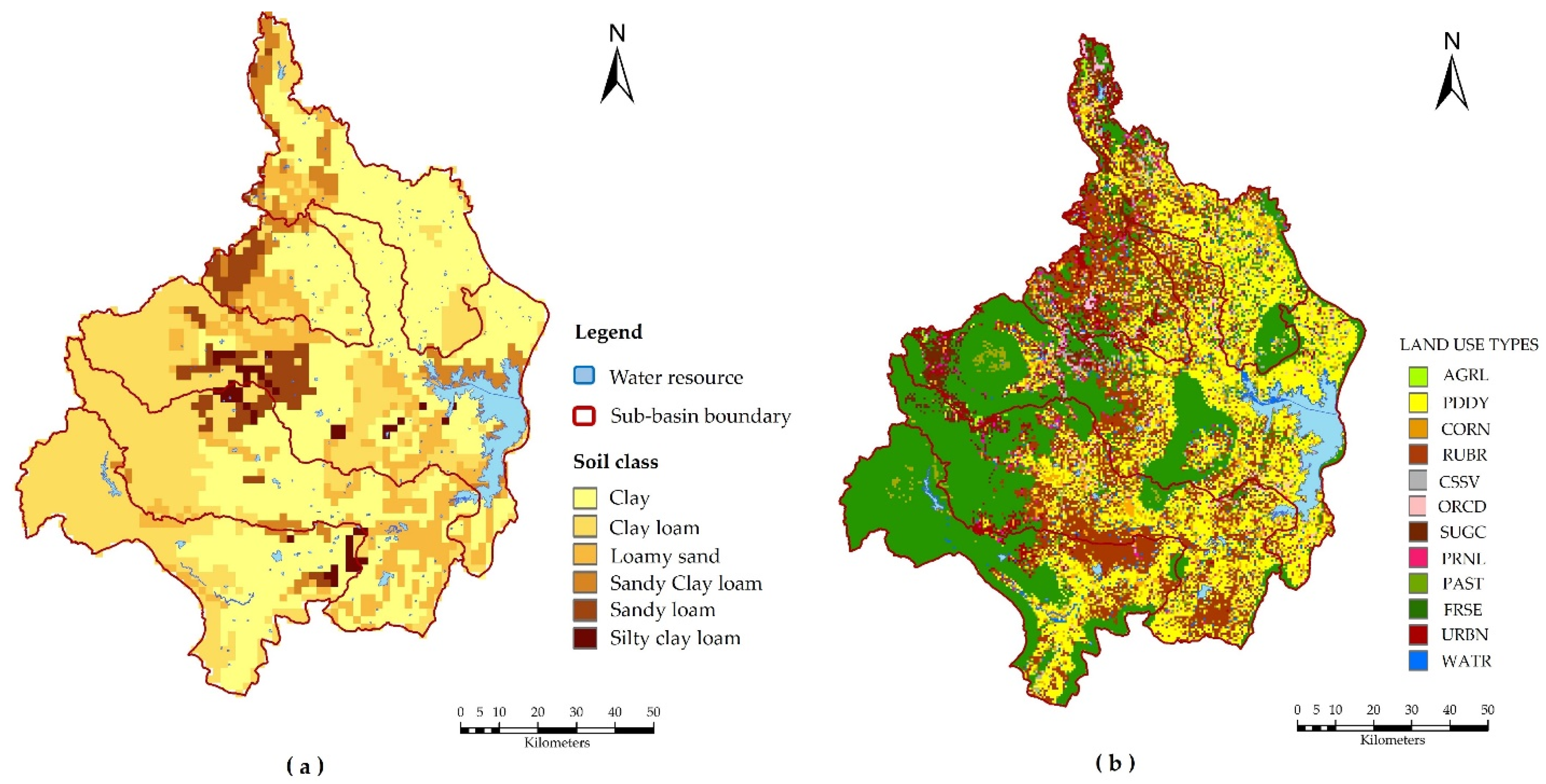
The SWAT (Soil and Water Assessment Tool) model was created to aid in the management of water resources, and it was utilized in the evaluations for estimating the impact of water resource management and water pollution in watersheds and large basins [36], the quantity of streamflow that has changed, the amount of sediment and water quality in streams affected by changes in land use and climate in both past, present and future projections [37], which could be divided into distinct stages of watershed processing. For example, in the main watershed, sub-watershed zones are being created. Calculations that demonstrate outcomes daily and at extended intervals are also included. This considers variables from hydrological processes with the water balance equation as in Equation (5).

$${\mathrm{SW}}_{\mathrm{t}}={\mathrm{SW}}_0+{\displaystyle \sum }_{\mathrm{i}=1}^{\mathrm{t}}\left({\mathrm{R}}_{\mathrm{day}}-{\mathrm{Q}}_{\mathrm{surf}}-{\mathrm{E}}_{\mathrm{a}}-{\mathrm{W}}_{\mathrm{seep}}-{\mathrm{Q}}_{\mathrm{gw}}\right)$$

(5)

where SW_t is the final soil water content; SW₀ is the initial soil water content, t is the time (days), R_day is the precipitation (mm) on the day i, Q_surf is the surface water content on the day I, E_a is the evaporative transpiration amount on the day I, W_seep is the amount of water seeping into the basement on the day i, and Q_gw is the amount of groundwater returning to the stream on the day i.

2.3.1. Data Input

In the implementation process, the SWAT method requires the import of basic physical data, including a digital elevation model (DEM) with elevation values between 90 to 1596 m (MSL). The watershed area has a slope from the west (mainly mountains and upstream forests) to the eastern lowland area where the Ubolratana Reservoir is located (see Figure 1). As for the soil type map (Figure 2a), it indicates that more than 50% of the soil is clay, which is in the eastern lowland, followed by clay loam soil, which is mainly in the eastern lowland of the study area. The types of land use in the study area were mostly agricultural areas. It was found that the use of land for rice farming which is most distributed in the eastern lowland area, combined with sugarcane and cassava plantation in the central area of the basin. In the west, most areas are watershed forests. The land use spatial distribution map is illustrated in Figure 2b.

Daily climate data includes rainfall, temperature, humidity, wind speed, and solar intensity. Daily rainfall data were collected from 9 rain gauge stations distributed in the study area and 1 climate station (Khon Kaen station) located in the southeastern part of the watershed, as shown in Figure 1. There are 4 stations of streamflow and sediment data, of which 3 stations are located in the watershed areas above the Ubolratana Reservoir, are Station E68A (Lam Pha Niang Basin), E29 Station (Upper Phong Basin), and E85 Station (Lam Chuan River). Basin). These data are from 2011–2019 supported by the Royal Irrigation Department of Thailand. The data used for evaluating the effectiveness of the SWAT-computed results for the different types, intervals, scales, and data sources used in this study are summarized and shown in

Table 1. Basic data to be used in the SWAT model.

Data Type	Period	Scale	Source
DEM	2015	30 × 30 m	Land Development Department, Thailand
Soil type map	2015	1:50,000
River map	2020	1:50,000
Land use map	2015	30 × 30 m
Climate	2011–2019	Daily	Thai Meteorological Department, Thailand
Observed inflow	2011–2019	Daily	Royal Irrigation Department, Thailand; Electricity Generating Authority, Thailand

.

2.3.2. Model Performance Evaluation Using SWAT-CUP

SWAT-CUP (SWAT Calibration and Uncertainty Procedure) is a SWAT-compatible model. When compared to the old approach of manual correction by trial and error, the SWAT model’s sensitive variable analysis, calibration, and validation procedures have more flexibility and take less time. The outcome of altering the sensitivity variable will serve as a guide for the best calibration and adjustment of the solution(s) between the SWAT generated results and the station data. The following are five approaches for determining the proper values: (1) Generalized Likelihood Uncertainty Estimation (GLUE), (2) Particle Swarm Optimization (PSO), (3) Parameter Solution (Parasol), (4) Mark Chain Monte Carlo (MCMC), and (5) Sequential Uncertainty Fitting (SUFI-2) [38]. For this study, the use of the SUFI-2 technique was selected to apply in the operation. The SUFI-2 technique is uncertainty analysis consisting of predictive P-factors representing the actual measured values that appear in the simulation results for 95% of the uncertainty of the simulation. The prediction (95% prediction uncertainty; 95PPU) and R-factor are calculated as the ratio of the mean amplitude range of the 95PPU to the standard variance of the actual data. The calculated 95PPU values were positioned at 2.5% and 97.5% of the cumulative probability distribution of the variables considered. Using Latin hypercube sampling [38] as this technique requires the least number of sensitivity variables but can produce the best results compared to other methods [39]. Eight parameters from the most vulnerable model types were chosen for examination in this study. Eight parameters from the most vulnerable model types were chosen for examination in this study. The results of the modification of the parameters that calculated streamflow from the model closest to the data from the measurement station are shown in

Table 2. Adjusted Model Sensitivity Parameters.

No.	Parameter	Range	Adjusted Values
1	ALPHA_BF.gw	0–1	0.367
2	GW_DELAY.gw	0–500	19.500
3	GWQMN.gw	0–500	179.500
4	ESCO.hru	0–1	0.881
5	GW_REVAP.gw	0–500	129.500
6	SOL_AWC.sol	0–1	0.393
7	CN2.mgt	−0.2–0.2	−0.104
8	EPCO.hru	0–1	0.819

.

Then, the results were compared with the data from the measurement station, and the efficiency was assessed using two statistical indices to check the accuracy of the results [40], which showed the level of accuracy of the monthly streamflow comparison results. It is divided into four levels as shown in

Table 3. Typical performance level for accepted statistics in monthly time step.

Level	R2	NSE
Very good	0.80 < R2 ≤ 1.00	0.75 < NSE ≤ 1.00
Good	0.70 < R2 ≤ 0.80	0.65 < NSE ≤ 0.75
Satisfactory	0.60 < R2 ≤ 0.70	0.50 < NSE ≤ 0.65
Unsatisfactory	R2 ≤ 0.60	NSE ≤ 0.50

[41].

• The Coefficient of Determination (R²), as shown in Equation (6), is between 0–1, with values greater than 0.6 indicating that the two data are correlated at a level of reliability.
• The Nash Sutcliffe efficiency (NSE) coefficient, as shown in Equation (7), is between −$\infty$ and 1, with values greater than 0.5 indicating that the two data are correlated at a level of reliability.

$${\mathrm{R}}^2={\left[\left(\frac{{\sum }_{\mathrm{i}=1}^{\mathrm{n}}\left({\mathrm{Q}}_{\mathrm{oi}}-{\mathrm{Q}}_{\mathrm{oa}}\right)\left({\mathrm{Q}}_{\mathrm{si}}-{\mathrm{Q}}_{\mathrm{sa}}\right)}{\sqrt{{\sum }_{\mathrm{i}=1}^{\mathrm{n}}{({\mathrm{Q}}_{\mathrm{oi}}-{\mathrm{Q}}_{\mathrm{oa}})}^2}\sqrt{{\sum }_{\mathrm{i}=1}^{\mathrm{n}}{({\mathrm{Q}}_{\mathrm{si}}-{\mathrm{Q}}_{\mathrm{sa}})}^2}}\right)\right]}^2$$

(6)

$${\mathrm{E}}_{\mathrm{ns}}=1-\left(\frac{{\sum }_{\mathrm{i}=1}^{\mathrm{n}}{\left({\mathrm{Q}}_{\mathrm{o}}-{\mathrm{Q}}_{\mathrm{s}}\right)}^2}{{\sum }_{\mathrm{i}=1}^{\mathrm{n}}{\left({\mathrm{Q}}_{\mathrm{o}}-{\mathrm{Q}}_{\mathrm{sa}}\right)}^2}\right)$$

(7)

where n is the total number of data. Q_oi is the i-order value, Q_oa is the mean from all measurements, Q_si is the i-order model, Q_sa is the i-order value from all models, Q_s is the calculated value from the model, and Q_o is the measurement value.

2.4. Application of HBMO Algorithm for Reservoir Rule Curves Generation

2.4.1. HBMO Algorithm

The HBMO Algorithm is a hybrid search algorithm based on bee mating behavior. The biological bee breeding process is transformed into a mathematical modeling program. As a result, the phases in the adjustment process were properly outlined. Mating is the first step in algorithm development. Every queen bee makes a flight based on her power and speed throughout each mating flight. Equation (8) determines the likelihood of mating between individual male bees and queen bees. The likelihood of mating is high during the start of the mating flight when the queen bee’s velocity is high, or when a male bee is sufficiently numerous to mate, the probability of mating is high.

After the movement of the queen bees or after mating, energy, and speed decrease according to Equations (9) and (10). When all queen bees have completed a pairing flight, they begin to breed to achieve the required number of embryos. The queen bees are selected in proportion to the queen bee’s fitness and are artificially inseminated with sperm randomly selected from the queen bee’s sperm sac. The worker bees would be selected in proportion to their fitness to be used to improve larval outcomes. After the embryos were born, they would be sorted according to their fitness. The best larvae replace the worst queen bees until there are no better embryos than any queen bees. The remaining larvae are then killed and new matings begin until there is a perfect mating. All predetermined will be completed or meet converging criteria [42].

$$Prob \left(Q,D\right)=e^{-\frac{\mathsf{\Delta }\left(f\right)}{S\left(t\right)}}$$

(8)

where $Prob \left(Q,D\right)$ is the probability of mating between the male bee $D$ and the queen bee $Q$ or the probability of successful mating; $\mathsf{\Delta }\left(f\right)$ is the difference between the male bee’s fitness (f(D)) and the fitness of the queen bee (f(Q)); S(t) is the speed of the queen bee at the time.

$$E\left(t+1\right)=E\left(t\right)-\gamma$$

(9)

$$S\left(t+1\right)=\alpha \times S\left(t\right)$$

(10)

where $E\left(t\right)$ is the queen’s energy; $S\left(t\right)$ is the queen’s speed; α is a factor ∈ [0, 1] and γ is the amount of energy reduction after each transition.

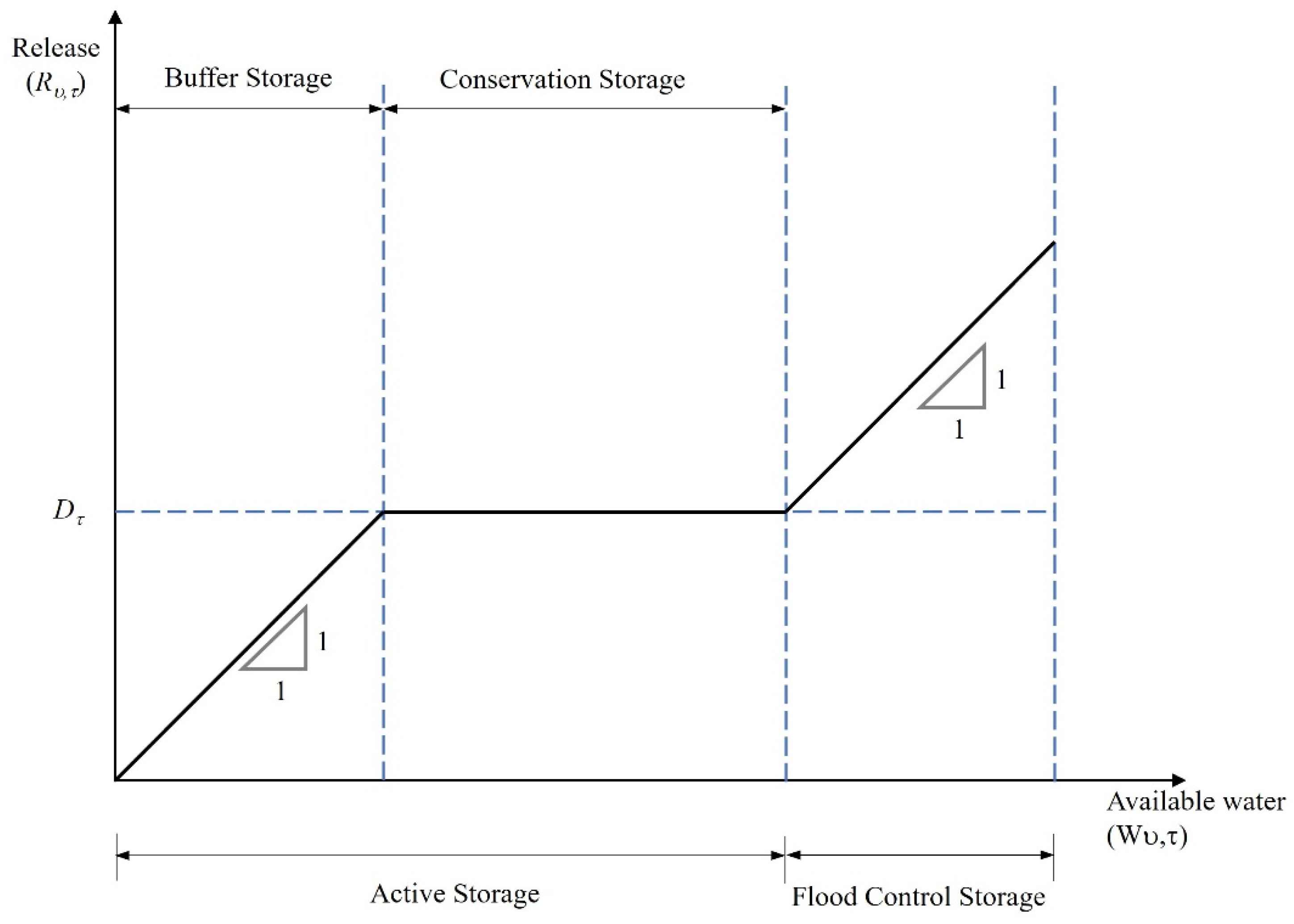
2.4.2. Water Equilibrium Simulation Model

The models HEC-3, HEC-5, and HEC-RAS were used in a simulation study of the reservoir system in each watershed [43]. Water balance principles were used. In this study, a simulation model of the reservoir system was created by using the same principles as in the above model, to facilitate connection with the Honey Bee Mating Optimization and begin calculating the water balance of each reservoir. To begin calculating the water balance of each reservoir from the rule curves, the initial storage volume of the reservoir was set at full capacity or the maximum storage level; the discharge volume could be calculated following the Standard Operating Rule as shown in Figure 3 and Equation (11). Then, the available water cost of the reservoir could be calculated for the next month with the principles of the water balance equation as shown in Equation (12).

$$R_{\nu ,\tau }=\{\begin{array}{c}{D}_{\tau }+W_{\nu ,\tau }-y_{\tau }, for W_{\nu ,\tau }\ge y_{\tau }+D_{\tau }\\ D_{\tau }, for x_{\tau }\le W_{\nu ,\tau }<y_{\tau }+D_{\tau }\\ D_{\tau }+W_{\nu ,\tau }-x_{\tau }, for x_{\tau }-D_{\tau }\le W_{\nu ,\tau }<x_{\tau }\\ 0, otherwise\end{array}$$

(11)

where R_υ,τ is the amount of water discharged from the reservoir during the year υ in the month τ (τ is 1 to 12 referring to January to December); D_τ is the demand for water at the bottom of the basin during month τ; x_τ is the lower boundary of the rule curves of the month τ; y_τ the upper boundary of the rule curves of the month τ; and W_υ,τ is the amount of original water level available in the basin of the month τ.

$$W_{\nu ,\tau +1}=S_{\nu ,\tau }+Q_{\nu ,\tau }-R_{\nu ,\tau }-E_{\tau }-DS$$

(12)

where S_υ,τ is the amount of water stored in the reservoir at the end of the month τ; Q_υ,τ is the average streamflow in the month τ; Eτ is the evaporation loss in the month τ; and DS (dead storage) is unused storage volume.

The reservoir rule curves were generated using the HBMO Algorithm Optimal Solution in this study. In the instance of shortage frequency, the target function for determining the solution was the least average shortage, as illustrated in Equation (13).

$$Min\left(Ave{r}_{Sh}\right)=\frac{1}{n}\sum _{v=1}^{n}S{h}_v$$

(13)

where $n$ is the length of the original water quantity data set; $S{h}_v$ is the amount of water shortage in the year $v$ (The amount of water released is less than the water demand target).

2.4.3. Reservoir Rule Curves Efficiency Evaluation

By analyzing the frequency of occurrence of an incident, the rule curves assessment was set to evaluate two parts: water scarcity and excess release water with mean and maximum values of Magnitude and Duration through the performances of the test rule curves with future monthly streamflow scenarios from 2020 to 2049. Changes in greenhouse gas emissions are RCP4.5 and RCP8.5, which are two different types of RCP.

3. Results and Discussion

3.1. Streamflow Analysis Using the SWAT Model

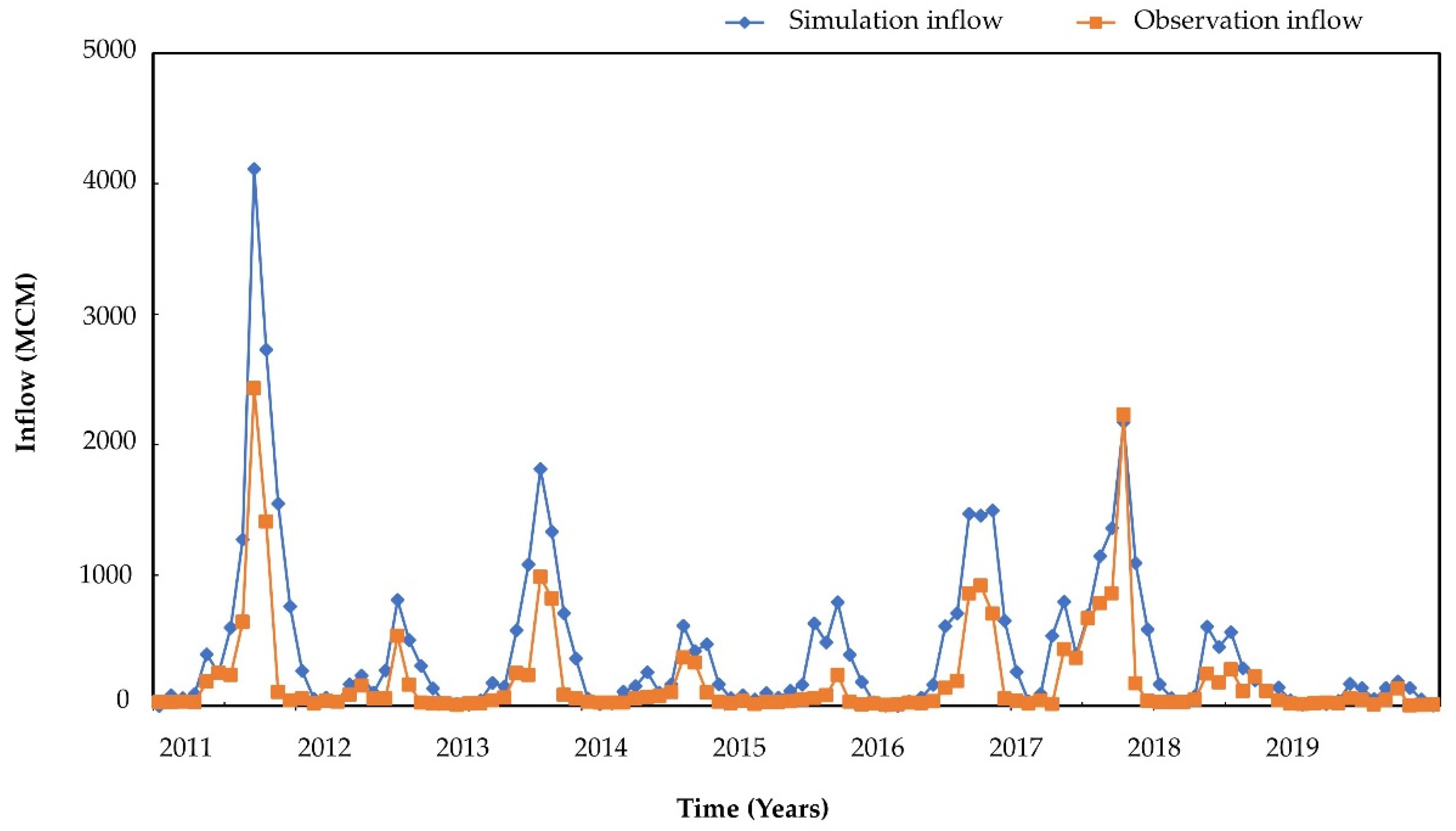
3.1.1. Model Performance Assessment

Evaluation of model performance assessed the accuracy between the calculation of streamflow from the SWAT model calculated from the average monthly streamflow volume during 2011–2019 and the streamflow data from 4 measurement stations in the study areas, namely E68A Station (Lam Pha Niang River Basin), E29 Station (Upper Phong River Basin), Ubolratana Dam Station, and E85 Station (Lam Nam Choen River Basin) in the same period. The model’s performance was evaluated using an index of R² ranging from 0.62–0.88 and NSE between 0.50–0.81, which were both within the acceptable accuracy range as shown in

Table 4. Index values for evaluating the accuracy of SWAT calculation results comparing streamflow volumes from measurement stations.

Assessment Index	R2	NSE
E68A Station (Lam Pha Niang River Basin)	0.82	0.52
E29 Station (Upper Phong River Basin)	0.79	0.76
Ubolratana Dam Station	0.88	0.81
E85 Station (Lam Nam Choen River Basin)	0.62	0.50

.

Comparative results of streamflow volumes from the SWAT model and streamflow data from Ubolratana Dam Station are shown in Figure 4. The average annual streamflow from the SWAT model is 5147.34 MCM and that of the measurement station is 2385.56 MCM.

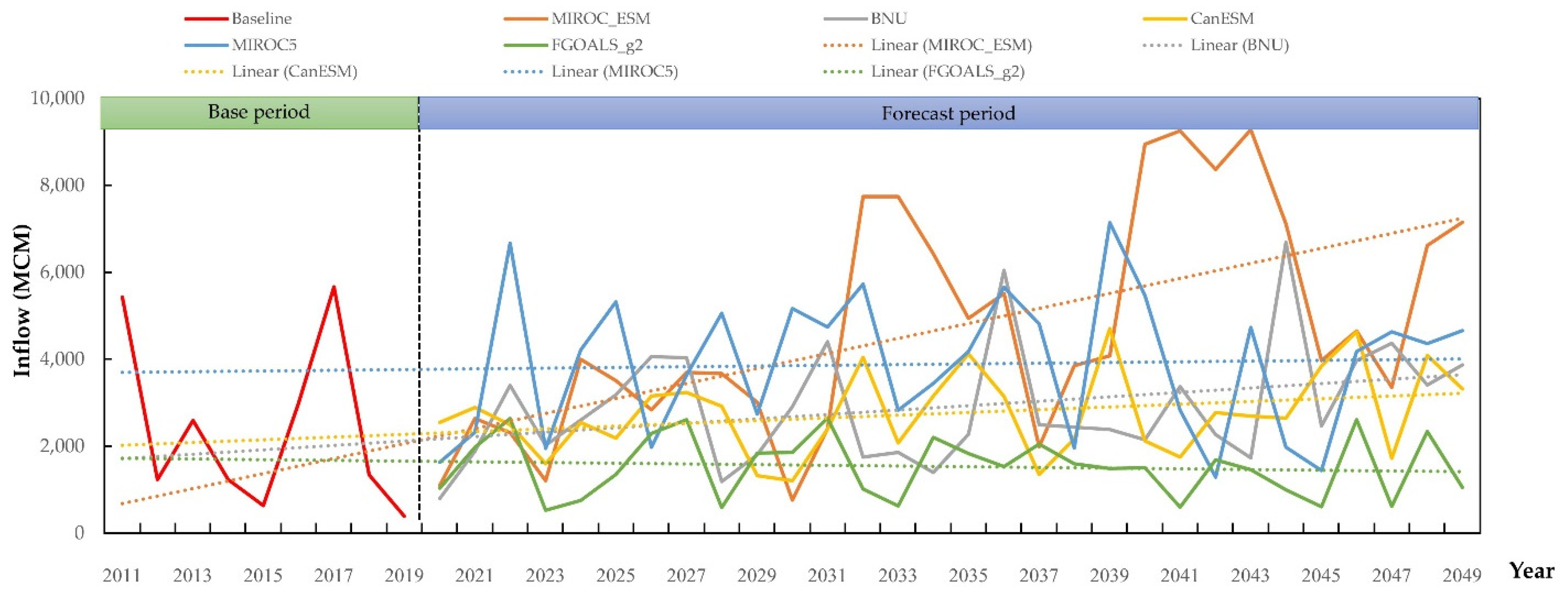
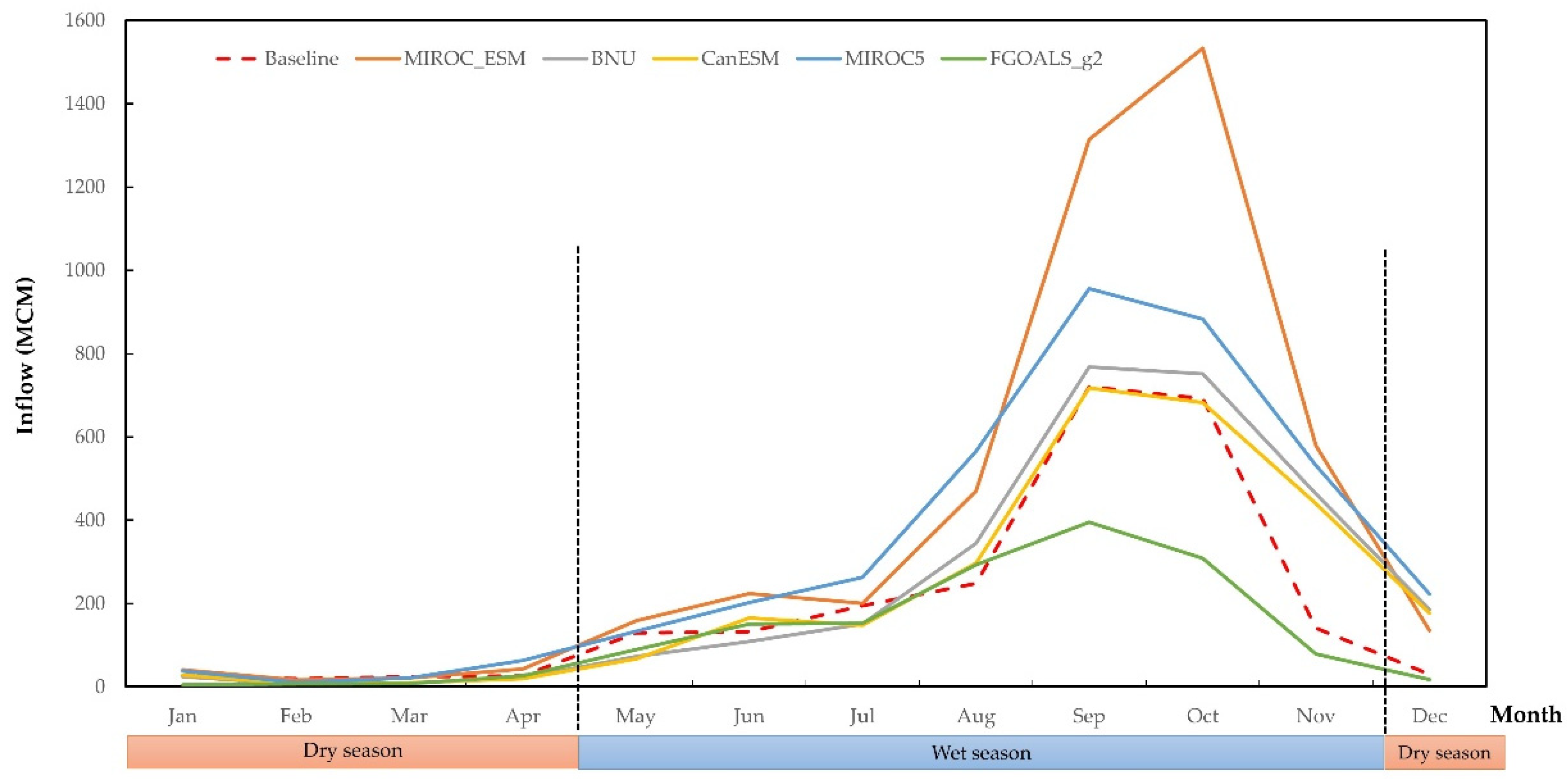
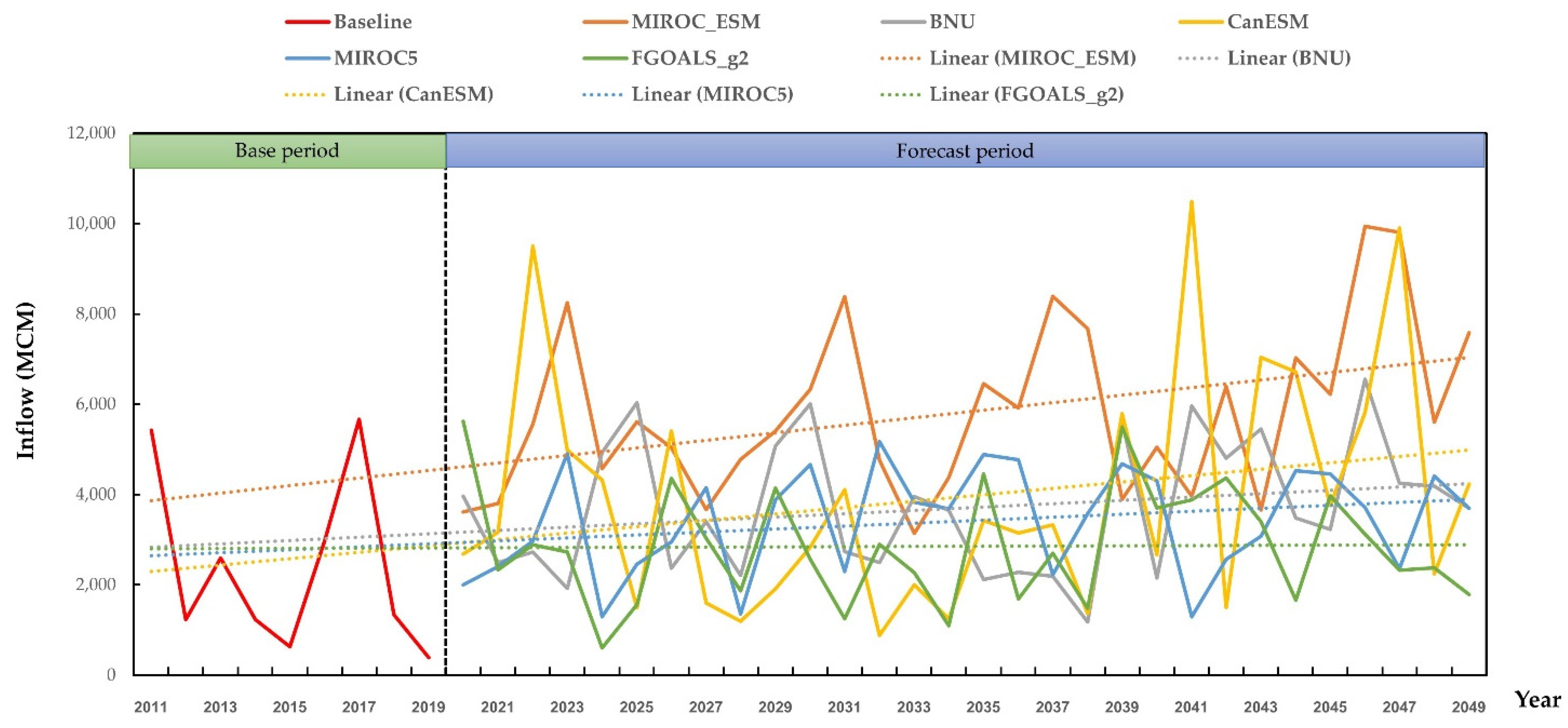
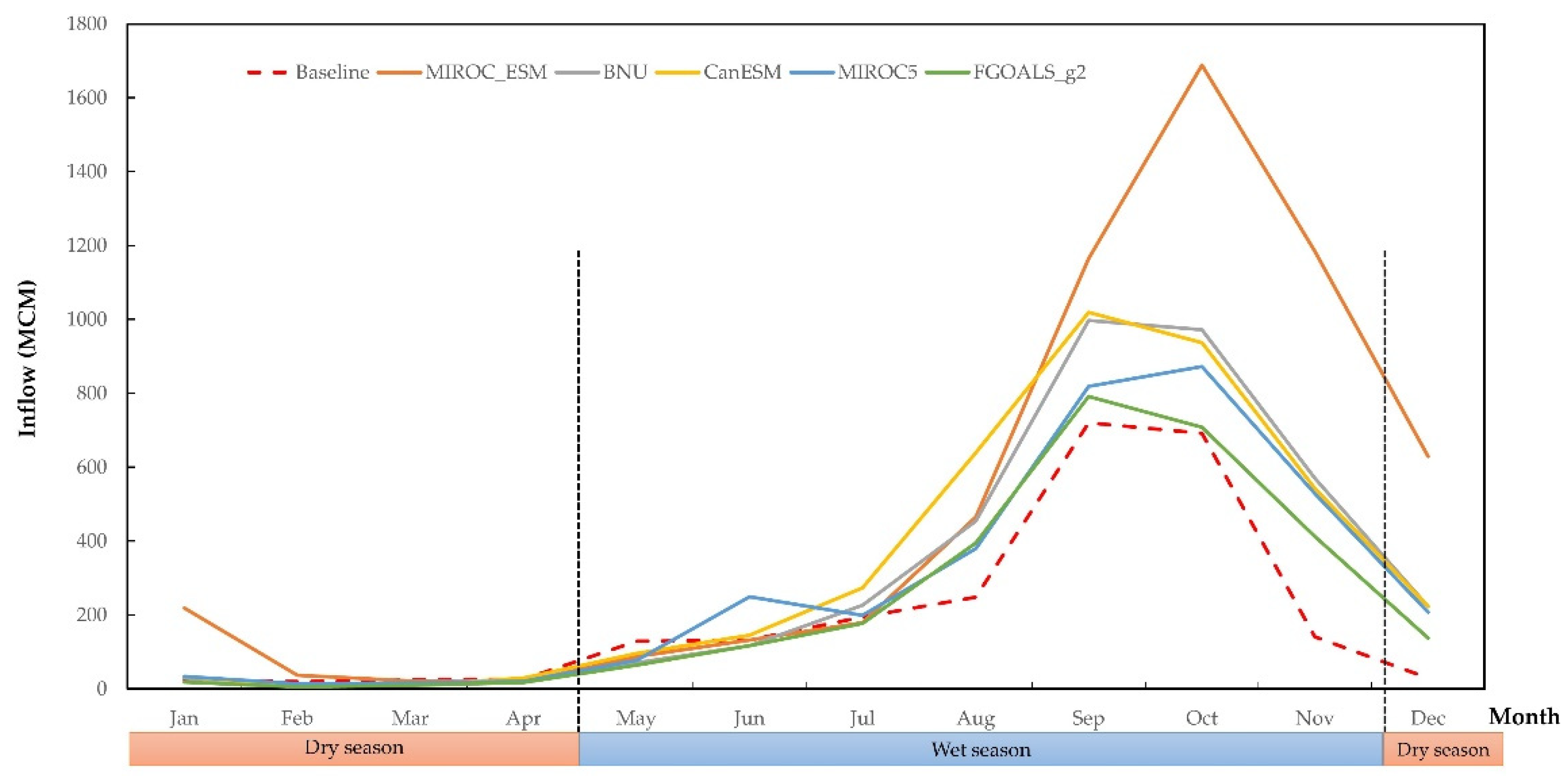
3.1.2. Forecasting of Future Streamflow Volumes

Forecasted future streamflow from 2020 to 2049 were expected to be impacted by climate change based on the CIMP5 model under the RCP4.5 projection case. In total, there was a 32% increase in the average annual streamflow in the future. With the MIROC_ESM model, the streamflow volume was likely to increase to a maximum of 4734.97 MCM (98.49%), and with the MIROC5 model, it was expected to rise by 3889.10 MCM (63.03%). In the BNU model, it increased to 2905.53 MCM (21.80%), and in the CanESM model, it increased to 2758.80 MCM (15.65%). However, the FGOALS_g2 model indicated that the average annual streamflow in the future was expected to decrease by 1528.95 MCM (−35.91%) (Figure 5). It was found that, overall, the average monthly streamflow volume increased during the rainy season, accounting for 2930.95 MCM (29.82%), and in the dry season, it accounted for 232.53 MCM (81.82%). When considering each model, there were 4 models, MIROC_ESM, BNU, CanESM, and MIROC5. There was an increase in the average monthly streamflow during the rainy season between 2516.67–4479.10 MCM (11.47–98.40%), and the monthly average streamflow volume would increase significantly during the dry season, especially in October showing a significantly higher proportion (Figure 6). The highest increase in the MIROC5 model was 356.00 MCM (178.36%). However, the study from the FGOALS_g2 model expressed a trend of lower average monthly streamflow in both rainy and dry seasons which were 1467.22 MCM (−35.01%) and 61.73 MCM (−51.73%) respectively. The results were in line with the average annual streamflow (

Table 5. Average monthly base year streamflow and seasonal forecasts.

Period	RCP	GCM	May–November (Wet Season) (MCM)		December–April (Dry Season) (MCM)
			Average	Difference (%)	Average	Difference (%)
Baseline (2011–2019)			2257.67		127.89
2020–2049	RCP4.5	Overall	2930.95	29.82	232.53	81.82
		MIROC_ESM	4479.10	98.40	255.87	100.07
		BNU	2658.62	17.76	246.90	93.06
		CanESM	2516.67	11.47	242.13	89.33
		MIROC5	3533.11	56.49	356.00	178.36
		FGOALS_g2	1467.22	−35.01	61.73	−51.73
	RCP8.5	Overall	3551.80	57.32	401.32	213.81
		MIROC_ESM	4902.41	117.14	926.05	624.11
		BNU	3409.38	51.01	294.67	130.41
		CanESM	3126.56	38.49	293.06	129.15
		MIROC5	3654.94	61.89	304.12	137.80
		FGOALS_g2	2665.69	18.07	188.71	47.56

).

Climate change was projected to influence future streamflow levels between 2020 and 2049, according to the CIMP5 model under the RCP8.5 forecast. The results showed that the average annual streamflow across all models tended to increase. The MIROC5 model rose by 5828.46 MCM (144.32%), the BNU model climbed by 3704.05 MCM (55.27%), and the CanESM model increased by 3704.05 MCM (55.27%) (55.27%). Model FGOALS_g2 grew to 2854.40 MCM (19.65%) and 3419.62 MCM (43.35%) (Figure 7). Looking at the seasonal average monthly streamflow volumes, the trend of change in average monthly water volume was similar under the RCP4.5 projection case but had a greater proportion of increase. Overall, the average monthly streamflow volume increased during the rainy season by 3551.80 MCM (57.32%) and by 401.32 MCM (213.81%) in the dry season. The increase was significant in both the rainy and dry seasons compared to the other models (Table 5), with a significant increase in percentage in October (Figure 8).

3.2. Optimal Reservoir Rule Curves with HBMO Algorithm Technique

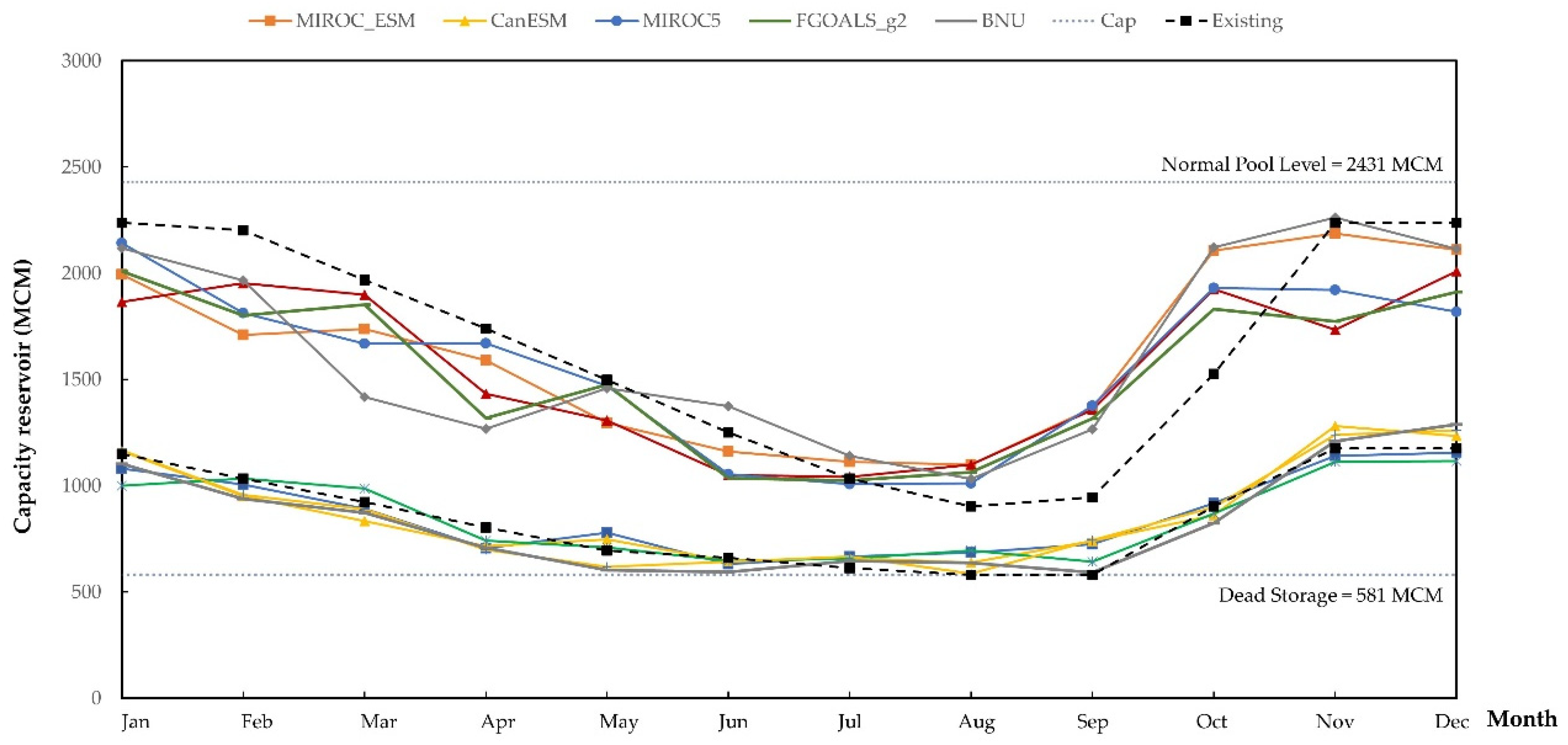
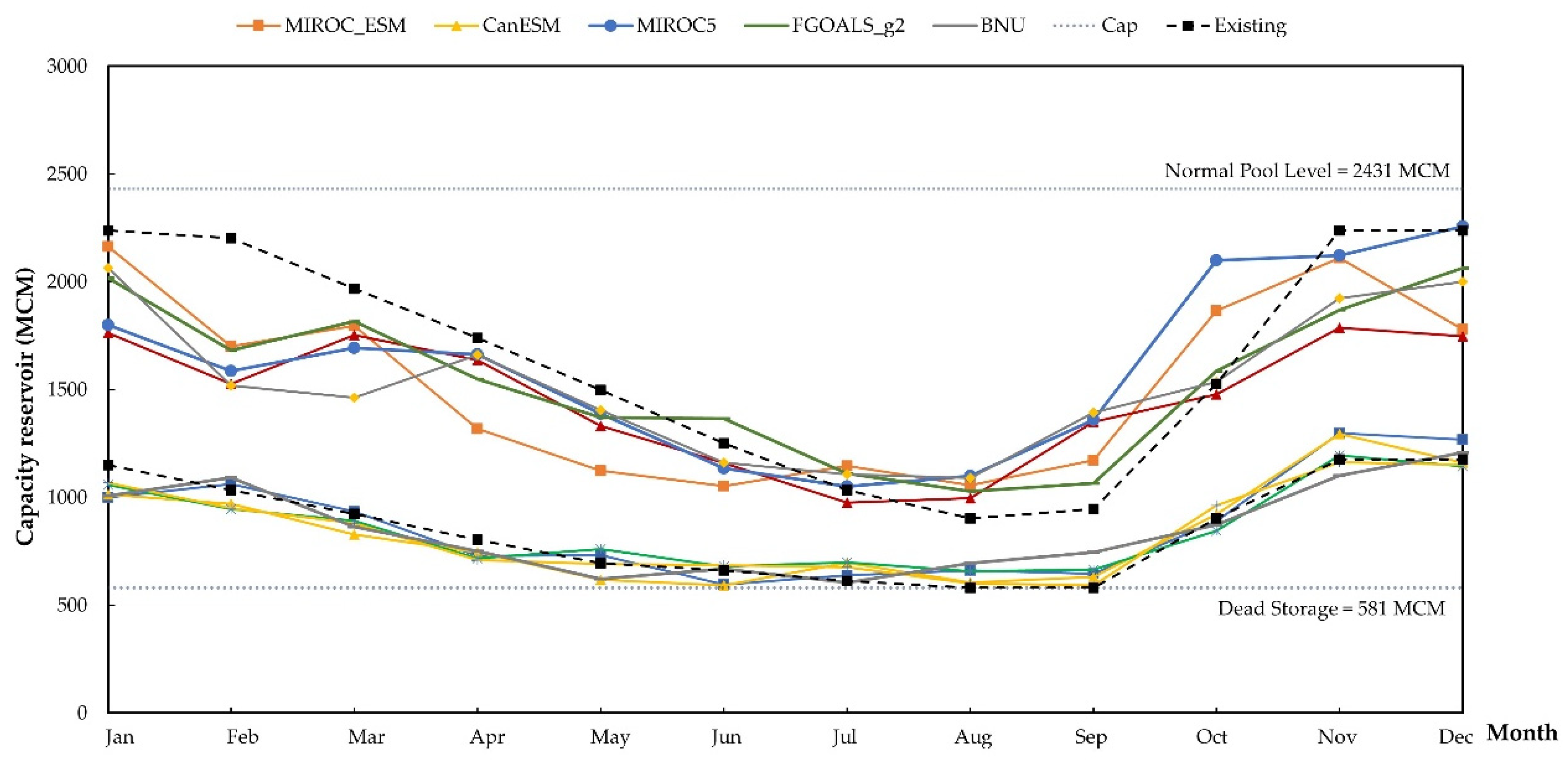
3.2.1. Optimal Reservoir Rule Curves by HBMO Algorithm

The findings of the Ubolratana Reservoir rule curves generated with the HBMO Algorithm approach based on the CIMP5 climate change impacts of 5 models under RCP4.5 and RCP8.5 projection cases were compared to the present Ubolratana Reservoir rule curves. The rule curves in both predicted situations were discovered to be identical to the existing rule curves. However, from July to September, the newly developed upper rule curves were higher than the current rule curves. This effected an increase in the amount of water stored in the reservoir, resulting in a sufficient water supply for the next dry season. In the upper rule curves of the two forecast cases, the shape corresponded to the current rule curves, but the lower rule curves developed lower than the current ones during the dry season from December to April. This means that the reservoir can release more water than with the current rule curves. It can reduce water scarcity, making it possible to respond to water users in irrigated areas (Figure 9 and Figure 10). According to recent study, applying the Harris Hawks Optimization (HHO) technique for searching in the Ubolratana reservoir, Thailand, the optimal rule curves with the HHO technique was similar to the current rule curves. The upper rule curves developed were higher than the current rule curves throughout the rainy season, allowing for additional water storage at the end of the rainy season [44].

3.2.2. Reservoir Rule Curves Efficiency Evaluation

The purpose of evaluating the efficiency of reservoir rule curves is to test the functions of the rule curves in order to know the results that could support the changing water situations due to various uncertainties, whether in past periods or for scenarios that may occur in the future. The assessment of rule curves had two parts, namely, water shortage and excess release water by assessing the frequency of occurrence of an incident through mean and maximum values of Magnitude and Duration.

We evaluated the efficiency of the current reservoir rule curves and the reservoir rule curves obtained from future streamflow during 2020–2049, which yielded five CIMP5 models of climate change under the RCP4.5 scenario. In all models except the MIROC5 model, the reservoir rule curves were able to lower the mean water deficit and mean overflow when compared to the present rule curves. Under the RCP4.5 scenario, the reservoir rule curves from the MIROC_ESM model were the most efficient ones in reducing mean water deficit and mean overflow when compared to the reservoir rule curves in other models (

Table 6. Estimated results of water shortage and overflow events of the Ubolratana reservoir rule curves from the MIROC_ESM model under the RCP4.5 projection case.

Situations	Rule Curves	Frequency (Times/Year)	Magnitude (MCM/Year)		Duration (Year)
			Average	Maximum	Average	Maximum
Water shortage	Existing	0.2	23.43	478.00	1.7	2.0
	MIROC_ESM	0.1	10.93	215.00	1.5	2.0
	BNU	0.1	14.87	264.00	2.0	2.0
	CanESM	0.1	14.17	295.00	1.5	2.0
	MIROC5	0.1	21.90	351.00	1.3	2.0
	FGOALS_g2	0.1	13.97	268.00	2.0	2.0
Excess water release	Existing	1.0	3235.04	8570.84	14.5	19.0
	MIROC_ESM	1.0	3181.27	8213.26	14.5	26.0
	BNU	1.0	3187.92	8124.91	14.5	26.0
	CanESM	1.0	3204.33	8284.15	14.5	19.0
	MIROC5	1.0	3216.58	8551.56	30.0	30.0
	FGOALS_g2	1.0	3207.96	8585.07	14.5	26.0

). Under the RCP8.5 scenario, the results showed that the reservoir rule curves in all models were able to reduce the average water shortage compared to the current rule curves. Moreover, the reservoir rule curves from the MIROC5 model could also help reduce the over-average water flow. The efficiency evaluation indicated that the reservoir rule curves from the MIROC5 model were able to reduce the average water shortage and average overflow the best when compared to the reservoir rule curves of all models (

Table 7. Estimated water shortage and overflow events of the Ubolratana reservoir rule curves from the MIROC5 model under the RCP8.5 projection case.

Situations	Rule Curves	Frequency (Times/Year)	Magnitude (MCM/Year)		Duration (Year)
			Average	Maximum	Average	Maximum
Water shortage	Existing	0.23	36.67	449.00	1.40	2.00
	MIROC_ESM	0.17	13.90	233.00	1.67	2.00
	BNU	0.07	7.77	195.00	2.00	2.00
	CanESM	0.13	12.77	259.00	2.00	2.00
	MIROC5	0.10	7.13	169.00	1.50	2.00
	FGOALS_g2	0.17	16.00	250.00	1.67	2.00
Excess water release	Existing	0.97	2460.08	6281.34	14.5	21
	MIROC_ESM	0.93	2460.26	5983.39	14	20
	BNU	0.87	2441.62	6165.43	8.667	15
	CanESM	0.93	2466.88	6055.38	9.333	15
	MIROC5	0.87	2424.31	6436.28	8.667	15
	FGOALS_g2	0.93	2452.14	6098.75	14	20

).

4. Conclusions

There were two primary objectives of this research. The first was to investigate how global climate change has affected the quantity of streamflow that flows into the Ubolratana Reservoir in the years 2020–2592. Second, these modifications will be utilized as data for improving the suitable reservoir rule curves using the HBMO algorithm approach, as well as evaluating the effectiveness of the newly designed reservoir rule curves.

The results of this study showed that future streamflow data are based on the SWAT model. The forecast years 2020–2049 were projected to be influenced by climate change from the CIMP5 model, according to the findings of this study. Both RCP4.5 and RCP8.5 were expected to rise under the anticipated conditions. Under RCP4.5 and RCP8.5, the future overall average annual streamflow will rise by 32% and 65%, respectively. The MIROC_ESM model had the highest average annual streamflow compared to other models. However, there is a different study (FGOALS_g2 model, under the RCP4.5 forecast case), which indicates that the future annual mean streamflow tends to decline. When we considered the average monthly streamflow volume in the future according to seasons, it was found that the trend of change in streamflow volume was consistent with both under the forecasting cases. The average monthly streamflow volume was expected to increase markedly during the wet season (August to November) and at the beginning of the dry season (December).

Then, the Ubolratana Reservoir rule curves developed by HBMO Algorithm was created. There were five CIMP5 climate models under the RCP4.5 and 8.5 forecast cases, for which the developed rule curves were shaped in accordance with the current rule curves. Moreover, the developed rule curves could also allow the reservoir to hold more water during the rainy season. This should ensure that there will be enough water in the next dry season. In addition, during the dry season, reservoirs will be able to release more water, thereby reducing water scarcity. Finally, the future rule curves in the reservoir as a result of the climate change examined in this study would be able to answer the objective functions, which is to acquire the least average water scarcity amount. The rule curves will also be rated for their efficiency in reducing water scarcity and overflow compared to the current rule curves.

References

1. Ehsani, N.; Vörösmarty, C.J.; Fekete, B.M.; Stakhiv, E.Z. Reservoir operations under climate change: Storage capacity options to mitigate risk. J. Hydrol. 2017, 555, 435–446. [Google Scholar] [CrossRef]
2. Ehteram, M.; Mousavi, S.F.; Karami, H.; Farzin, S.; Singh, V.P.; Chau, K.W.; El-Shafie, A. Reservoir operation based on evolutionary algorithms and multi-criteria decision-making under climate change and uncertainty. J. Hydroinform. 2018, 20, 332–355. [Google Scholar] [CrossRef]
3. Gorguner, M.; Kavvas, M.L. Modeling impacts of future climate change on reservoir storages and irrigation water demands in a Mediterranean basin. Sci. Total Environ. 2020, 748, 141246. [Google Scholar] [CrossRef] [PubMed]
4. Abera, F.F.; Asfaw, D.H.; Engida, A.N.; Melesse, A.M. Optimal operation of hydropower reservoirs under climate change: The case of Tekeze reservoir, Eastern Nile. Water 2018, 10, 273. [Google Scholar] [CrossRef] [Green Version]
5. Carvalho-Santos, C.; Monteiro, A.T.; Azevedo, J.C.; Honrado, J.P.; Nunes, J.P. Climate change impacts on water resources and reservoir management: Uncertainty and adaptation for a mountain catchment in northeast Portugal. Water Resour Manag. 2017, 31, 3355–3370. [Google Scholar] [CrossRef] [Green Version]
6. Moazzam, M.F.; Lee, B.G.; Rahman, G.; Waqas, T. Spatial Rainfall Variability and an Increasing Threat of Drought, According to Climate Change in Uttaradit Province, Thailand. Atmos. Clim. Sci. 2020, 10, 357. [Google Scholar] [CrossRef]
7. Tebakari, T.; Dotani, K.; Kato, T. Historical change in the flow duration curve for the upper nan River Watershed, Northern Thailand. J. Jpn. Soc. Hydrol. Water Resour. 2018, 31, 17–24. [Google Scholar] [CrossRef] [Green Version]
8. Sharma, D.; Babel, M.S. Assessing hydrological impacts of climate change using bias-corrected downscaled precipitation in Mae Klong basin of Thailand. Meteorol. Appl. 2018, 25, 384–393. [Google Scholar] [CrossRef]
9. Petpongpan, C.; Ekkawatpanit, C.; Kositgittiwong, D. Climate change impact on surface water and groundwater recharge in Northern Thailand. Water 2020, 12, 1029. [Google Scholar] [CrossRef] [Green Version]
10. Kamworapan, S.; Surussavadee, C. Evaluation of CMIP5 global climate models for simulating climatological temperature and precipitation for Southeast Asia. Adv. Meteorol. 2019, 2019, 1067365. [Google Scholar] [CrossRef]
11. Bhatta, B.; Shrestha, S.; Shrestha, P.K.; Talchabhadel, R. Evaluation and application of a SWAT model to assess the climate change impact on the hydrology of the Himalayan River Basin. Catena 2019, 181, 104082. [Google Scholar] [CrossRef]
12. Azari, M.; Oliaye, A.; Nearing, M.A. Expected climate change impacts on rainfall erosivity over Iran based on CMIP5 climate models. J. Hydrol. 2021, 593, 125826. [Google Scholar] [CrossRef]
13. Saharia, A.M.; Sarma, A.K. Future climate change impact evaluation on hydrologic processes in the Bharalu and Basistha basins using SWAT model. Nat. Hazards 2018, 92, 1463–1488. [Google Scholar] [CrossRef]
14. Chuenchooklin, S.; Pangnakorn, U. Hydrological Study Using SWAT and Global Weather, a Case Study in the Huai Khun Kaeo Watershed in Thailand. Int. J. Environ. Prot. Pol. 2018, 6, 36. [Google Scholar] [CrossRef] [Green Version]
15. Prasanchum, H.; Sirisook, P.; Lohpaisankrit, W. Flood risk areas simulation using SWAT and Gumbel distribution method in Yang Catchment, Northeast Thailand. Geogr. Tech. 2020, 15, 29–39. [Google Scholar] [CrossRef]
16. Ekkawatpanit, C.; Pratoomchai, W.; Khemngoen, C.; Srivihok, P. Climate change impact on water resources in Klong Yai River Basin, Thailand. Proc. Int. Assoc. Hydrol. Sci. 2020, 383, 355–365. [Google Scholar] [CrossRef]
17. Thongwan, T.; Kangrang, A.; Techarungreungsakul, R.; Ngamsert, R. Future inflow under land use and climate changes and participation process into the medium-sized reservoirs in Thailand. Adv. Civ. Eng. 2020, 2020, 5812530. [Google Scholar] [CrossRef]
18. Prasanchum, H.; Kangrang, A. Optimal reservoir rule curves under climatic and land use changes for Lampao Dam using Genetic Algorithm. KSCE J. Civ. Eng. 2018, 22, 351–364. [Google Scholar] [CrossRef]
19. Kumar, N.; Singh, S.K.; Srivastava, P.K.; Narsimlu, B. SWAT Model calibration and uncertainty analysis for streamflow prediction of the Tons River Basin, India, using Sequential Uncertainty Fitting (SUFI-2) algorithm. Model. Earth Syst. Environ. 2017, 3, 30. [Google Scholar] [CrossRef]
20. Abeysingha, N.S.; Islam, A.; Singh, M. Assessment of climate change impact on flow regimes over the Gomti River basin under IPCC AR5 climate change scenarios. J. Water Clim. Chang. 2020, 11, 303–326. [Google Scholar] [CrossRef]
21. Tayebiyan, A.; Mohammad, T.A.; Al-Ansari, N.; Malakootian, M. Comparison of optimal hedging policies for hydropower reservoir system operation. Water 2019, 11, 121. [Google Scholar] [CrossRef] [Green Version]
22. Akbarifard, S.; Sharifi, M.R.; Qaderi, K. Data on optimization of the Karun-4 hydropower reservoir operation using evolutionary algorithms. Data Br. 2020, 29, 105048. [Google Scholar] [CrossRef] [PubMed]
23. Kangrang, A.; Chaleeraktrakoon, C. Suitable Conditions of Reservoir Simulation for Searching Rule Curves. J. Appl. Sci. 2008, 8, 1274–1279. [Google Scholar] [CrossRef] [Green Version]
24. Kangrang, A.; Lokham, C. Optimal Reservoir Rule Curves Considering Conditional Ant Colony Optimization with. J. Appl. Sci. 2013, 13, 154–160. [Google Scholar] [CrossRef]
25. Kangrang, A.; Srikamol, N.; Hormwichian, R.; Prasanchum, H.; Sriwanphen, O. Alternative Approach of Firefly Algorithm for Flood Control Rule Curves. Asian J. Sci. Res. 2019, 12, 431–439. [Google Scholar] [CrossRef]
26. Sinthuchai, N.; Kangrang, A. Improvement of Reservoir Rule Curves using Grey Wolf Optimizer. J. Eng. Appl. Sci. 2019, 14, 9847–9856. [Google Scholar] [CrossRef] [Green Version]
27. Marchand, A.; Gendreau, M.; Blais, M.; Guidi, J. Optimized operating rules for short-term hydropower planning in a stochastic environment. Comput. Manag. Sci. 2019, 16, 501–519. [Google Scholar] [CrossRef]
28. Thongwan, T.; Kangrang, A.; Prasanchum, H. Multi-objective future rule curves using conditional tabu search algorithm and conditional genetic algorithm for reservoir operation. Heliyon 2019, 5, e02401. [Google Scholar] [CrossRef]
29. Haddad, O.B.; Afshar, A.; Mariño, M.A. Honey-bee mating optimization (HBMO) algorithm in deriving optimal operation rules for reservoirs. J. Hydroinform. 2008, 10, 257–264. [Google Scholar] [CrossRef]
30. Kangrang, A.; Prasanchum, H.; Hormwichian, R. Active future rule curves for multi-purpose reservoir operation on the impact of climate and land use changes. J. Hydro-Environ. Res. 2019, 24, 1–13. [Google Scholar] [CrossRef]
31. Ferguson, C.R.; Pan, M.; Oki, T. The effect of global warming on future water availability: CMIP5 synthesis. Water Resour. Res. 2018, 54, 7791–7819. [Google Scholar] [CrossRef]
32. Climate Change in Australia. List of Global Climate Models. Available online: https://www.climatechangeinaustralia.gov.au/en/overview/methodology/list-models/ (accessed on 20 February 2022).
33. Zhou, T.; Yu, Y.; Liu, Y.; Wang, B. (Eds.) Flexible Global Ocean-Atmosphere-Land System Model: A Modeling Tool for the Climate Change Research Community; Springer: Berlin/Heidelberg, Germany, 2014. [Google Scholar]
34. Chaowiwat, W. Impact of climate change assessment on agriculture water demand in Thailand. Naresuan Univ. Eng. J. 2016, 11, 35–42. [Google Scholar]
35. Sharma, D. Selection of suitable general circulation model precipitation and application of bias correction methods: A case study from the Western Thailand. In Environmental Management of River Basin Ecosystems; Springer: Cham, Switzerland, 2015; pp. 43–63. [Google Scholar]
36. Arnold, A.G.; Srinivasan, R.; Muttiah, R.S.; Williams, J.R. Large area hydrological modeling and assessment pert I: Model development. J. Am. Water Resour. Assoc. 1998, 34, 73–89. [Google Scholar] [CrossRef]
37. Prasanchum, H.; Kangrang, A. Analyses of climate and land use changes impact on runoff characteristics for multi-purpose reservoir system. In Proceedings of the Conference on The AUN/SEED-Net Regional Conference 2016 on Environmental Engineering (RC-EnvE 2016), Chonburi, Thailand, 23–24 January 2017. [Google Scholar]
38. Khalid, K.; Ali, M.F.; Abd Rahman, N.F.; Mispan, M.R.; Haron, S.H.; Othman, Z.; Bachok, M.F. Sensitivity analysis in watershed model using SUFI-2 algorithm. Procedia. Eng. 2016, 162, 441–447. [Google Scholar] [CrossRef] [Green Version]
39. Shivhare, N.; Dikshit, P.K.; Dwivedi, S.B. A comparison of SWAT model calibration techniques for hydrological modeling in the Ganga river watershed. Engineering 2018, 4, 643–652. [Google Scholar] [CrossRef]
40. Moriasi, D.N.; Gitau, M.W.; Pai, N.; Daggupati, P. Hydrologic and water quality models: Performance measures and evaluation criteria. Trans. ASABE 2015, 58, 1763–1785. [Google Scholar]
41. Zhang, S.; Li, Z.; Lin, X.; Zhang, C. Assessment of climate change and associated vegetation cover change on watershed-scale runoff and sediment yield. Water 2019, 11, 1373. [Google Scholar] [CrossRef] [Green Version]
42. Haddad, O.B.; Afshar, A.; Mariño, M.A. Honey-bees mating optimization (HBMO) algorithm: A new heuristic approach for water resources optimization. Water Resour. Manag. 2006, 20, 661–680. [Google Scholar] [CrossRef]
43. Rodriguez, L.B.; Cello, P.A.; Vionnet, C.A.; Goodrich, D. Fully conservative coupling of HEC-RAS with MODFLOW to simulate stream–aquifer interactions in a drainage basin. J. Hydrol. 2008, 353, 129–142. [Google Scholar] [CrossRef]
44. Techarungruengsakul, R.; Kangrang, A. Application of Harris Hawks Optimization with Reservoir Simulation Model Considering Hedging Rule for Network Reservoir System. Sustainability 2022, 14, 4913. [Google Scholar] [CrossRef]
Figure 1. Study areas of tributaries in the Chi River Basin.
Sustainability 14 08599 g001
Figure 2. Soil Type Map (a), Land use map (b).
Sustainability 14 08599 g002
Figure 3. Standard water discharge criteria.
Sustainability 14 08599 g003
Figure 4. Comparison of streamflow between the data from Ubolratana Dam Station and the calculated results from the SWAT model during 2011–2019.
Sustainability 14 08599 g004
Figure 5. Annual streamflow from the base year SWAT model 2011–2019 and under the forecast of RCP 4.5 between 2020–2049.
Sustainability 14 08599 g005
Figure 6. Monthly streamflow from the base year SWAT model 2011–2019 and under the forecast of RCP 4.5 between 2020–2049.
Sustainability 14 08599 g006
Figure 7. Annual streamflow from the base year SWAT model 2011–2019 and under the forecast of RCP 8.5 between 2020–2049.
Sustainability 14 08599 g007
Figure 8. Monthly streamflow from the base year SWAT model 2011–2019 and under the forecast of RCP 8.5 between 2020–2049.
Sustainability 14 08599 g008
Figure 9. Rule curves of Ubolratana reservoir developed using HBMO algorithm technique based on climate change impacts under the RCP4.5 projection case.
Sustainability 14 08599 g009
Figure 10. Rule curves of Ubolratana reservoir developed using HBMO algorithm technique based on climate change impacts under the RCP8.5 projection case.
Sustainability 14 08599 g010