
Residential Buildings’ Real Estate Values Linked to Summer Surface Thermal Anomaly Patterns and Urban Features: A Florence (Italy) Case Study

 , , and
Abstract
:1. Introduction
2. Materials and Methods
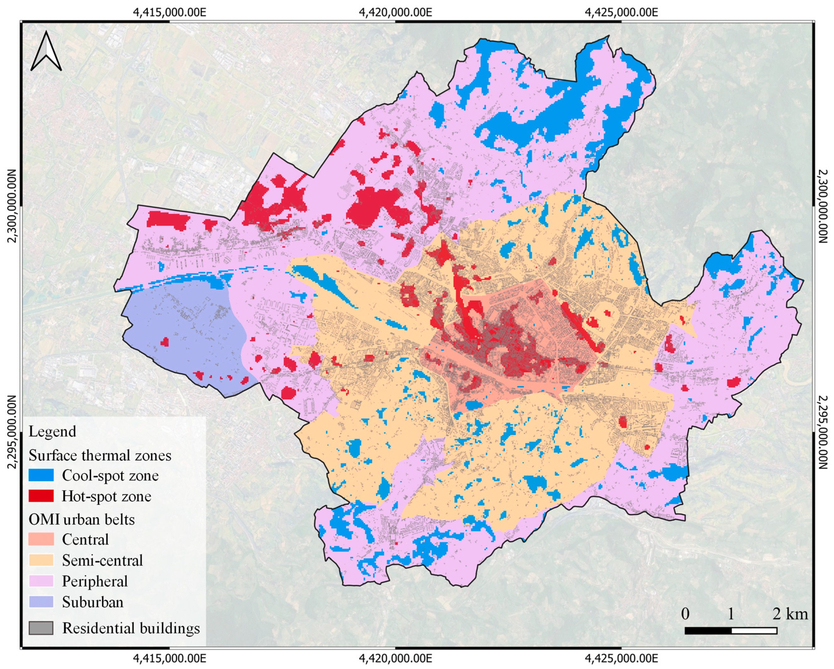
2.1. Study-Area
2.2. Study Framework and Methodological Approach
- Descriptive analyses concerning the characterization of residential buildings located in different urban areas based on the number, density, and dimension (area and volume) of residential building units, as well as including demographic (resident population and population density), surface (the average albedo and land surface temperature of residential building’s roofs), and morphological (Sky View Factor surrounding residential buildings) data.
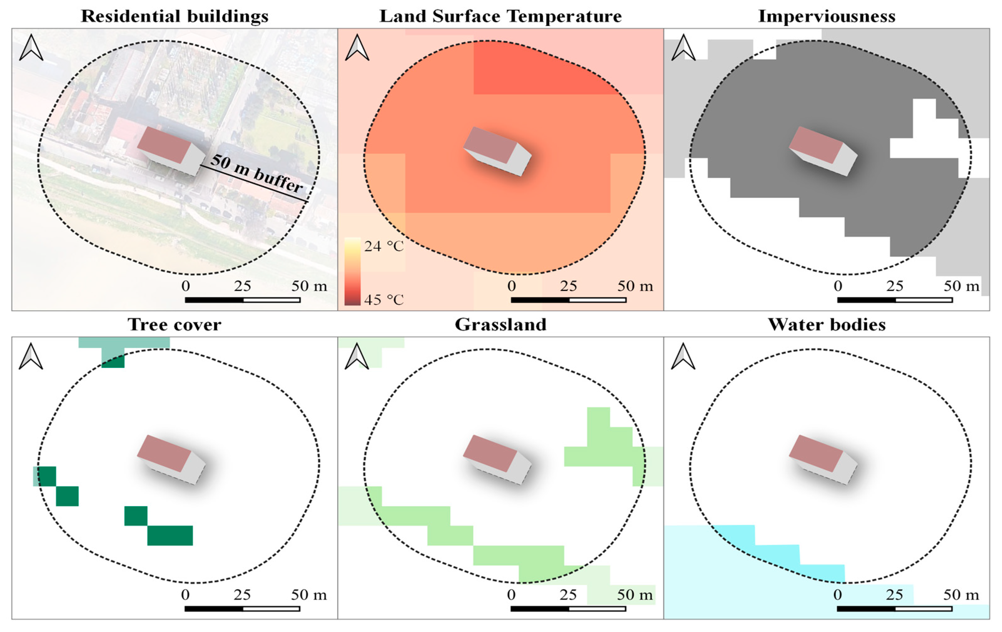
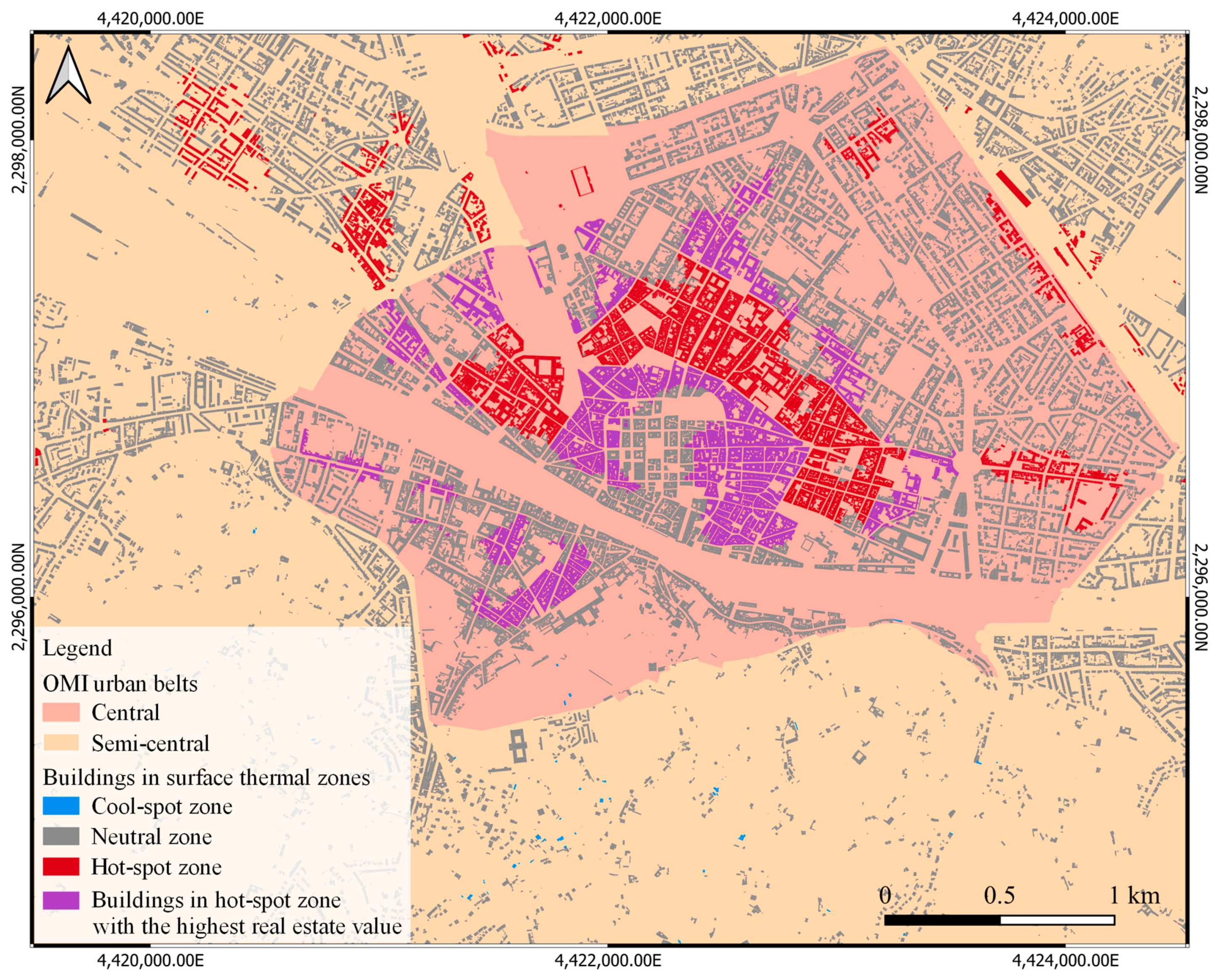
- Investigation of the relationships between residential buildings’ real estate values, surface thermal anomaly patterns, and urban green, blue, and grey infrastructures surrounding residential buildings, by considering two buffer areas with different sizes (50 m and 100 m). The buffer area was calculated following a homogeneous criterion starting from the perimeter of each residential building unit, with the aim of considering the surrounding characteristics proximal to residential buildings. Residential buildings falling into summer thermal hot- and cool-spot zones were investigated and compared with buildings falling in those thermally neutral.
2.3. Residential Buildings Real Estate Values
2.4. Characterization of Residential Buildings Located in Different OMI Belts
- Number, density, surface areas, and volumes of the residential building units from the 2011 census were extracted by the buildings database of the Tuscany Region (GEOscopio platform) by filtering the residential building category class;
- Resident population and population density data were provided by the Italian National Institute of Statistics (ISTAT, https://www.istat.it/en/, accessed on 7 June 2022), through the regional database of Tuscany (GEOscopio platform), referring to the year 2011;
- Land Surface Temperature (LST) of residential building roofs was obtained by using Landsat 8 TIRS (Thermal Infrared Sensor) remote sensing data resampled to 30 m horizontal resolution (the original resolution of TIRS bands was 100 m) by the U. S. Geological Survey (https://earthexplorer.usgs.gov/, accessed on 7 June 2022). LST was retrieved for clear-sky days (cloud cover < 5%) selected from June to August of the 2015–2019 daytime (09:58 UTC) summer period (June-July-August). Mean summer daytime LST was calculated by using all available images converted from Kelvin to Celsius degrees (°C) by the following method developed by the U.S. Geological Survey and also applied in previous studies on the same study-area [20,21] (Equations (1) and (2)):
- Surface albedo of residential building roofs was obtained by using Sentinel-2 Level 2A remote sensing product (10 m horizontal resolution) of the Copernicus mission (https://scihub.copernicus.eu/dhus/#/home, accessed on 7 June 2022), which referred to the 2017 daytime (from 10:00 to 11:00 UTC) summer period (from July to August), according to the method developed by a recent study [30]. The following Equations (3) and (4) were used to retrieve the surface broadband albedo (α) by considering the observed surface as Lambertian [30]:
- Sky View Factor (SVF) was obtained by the Digital Surface Model (1 m horizontal resolution, year 2017) in the QGIS environment by using 100 m radius and 16 search directions, as indicated in previous studies evaluating urban environments [31,32,33]. As suggested by previous studies, a 100 m radius was considered the best and most useful search area for urban studies. SVF values were averaged on each OMI belt with the aim to evaluate the urban morphology. The retrieval formula (Equation (5)) was used by considering the height of the obstacle (H) and the distance between obstacles (W) [34]:
2.5. Focus on Surface Thermal Anomaly Patterns and Urban Features
- a = buildings in hot-spot (or cool-spot) zones belonging to a specific OMI class (therefore OMI_C1, OMI_C2, OMI_C3 or OMI_C4);
- b = buildings in hot-spot (or cool-spot) zones belonging to other OMI classes;
- c = buildings in non-hot-spot (or cool-spot) zones belonging to a specific OMI class;
- d = buildings in non-hot-spot (or cool-spot) zones belonging to other OMI classes.
- green infrastructures, such as tree cover (TC), and grassland area (GA);
- blue infrastructure, such as water bodies (WB);
- grey infrastructure, such as impervious area (IA).
3. Results
3.1. Descriptive Analyses
3.2. Residential Buildings’ Real Estate Values-Related Urban Features
3.2.1. Relationships between Residential Buildings’ Real Estate Values and Surface Thermal Anomaly Patterns
3.2.2. Relationships between Real Estate Values and Urban Features Surrounding Residential Buildings
4. Discussion
Study Limitation
5. Conclusions
- What will happen to the real estate value of residential buildings falling into hot-spot zones if targeted actions are not planned?
- Will the attractiveness and charm of a residential building located in a historical, cultural, and architectural context be able to continue to prevail over the increasingly higher operational costs at real estate assets necessary to ensure a good quality of life in specific areas of the city characterized by significant temperature increases?
Supplementary Materials
Author Contributions
Funding
Institutional Review Board Statement
Informed Consent Statement
Data Availability Statement
Acknowledgments
Conflicts of Interest
Abbreviations
| LST | Land surface temperature |
| IA | Impervious area |
| TC | Tree cover |
| GA | Grassland area |
| WB | Water bodies |
| SVF | Sky View Factor |
| OMI | Real Estate Market Observatory of the National Revenue Agency of Italy |
| OMI_C | OMI zone classes: ranging from OMI_C1 to OMI_C4 with the lowest of the highest residential building real estate values, respectively |
References
- Hjort, J.; Streletskiy, D.; Doré, G.; Wu, Q.; Bjella, K.; Luoto, M. Impacts of permafrost degradation on infrastructure. Nat. Rev. Earth Environ. 2022, 3, 24–38. [Google Scholar] [CrossRef]
- World Meteorological Organization. The Global Climate in 2015–2019; World Meteorological Organization (WMO): Geneva, Switzerland, 2020. Available online: https://library.wmo.int/doc_num.php?explnum_id=10251 (accessed on 6 June 2022).
- Mirzaei, M.; Verrelst, J.; Arbabi, M.; Shaklabadi, Z.; Lotfizadeh, M. Urban Heat Island Monitoring and Impacts on Citizen’s General Health Status in Isfahan Metropolis: A Remote Sensing and Field Survey Approach. Remote Sens. 2020, 12, 1350. [Google Scholar] [CrossRef]
- Battaglia, J.M.A.; Douglas, S.; Hennigan, C.J. Effect of the Urban Heat Island on Aerosol pH. Environ. Sci. Technol. 2017, 51, 13095–13103. [Google Scholar] [CrossRef]
- Heaviside, C.; Macintyre, H.; Vardoulakis, S. The Urban Heat Island: Implications for Health in a Changing Environment. Curr. Environ. Health Rep. 2017, 4, 296–305. [Google Scholar] [CrossRef]
- Akbari, H.; Kolokotsa, D. Three decades of urban heat islands and mitigation technologies research. Energy Build. 2016, 133, 834–842. [Google Scholar] [CrossRef]
- Amirtham, L.R.; Devadas, M.D.; Perumal, M.; Amirtham, L. Mapping of Micro-Urban Heat Islands and Land Cover Changes: A Case in Chennai City, India. Int. J. Clim. Chang. Impacts Responses 2009, 1, 71–84. [Google Scholar] [CrossRef]
- Smargiassi, A.; Goldberg, M.S.; Plante, C.; Fournier, M.; Baudouin, Y.; Kosatsky, T. Variation of daily warm season mortality as a function of micro-urban heat islands. J. Epidemiol. Community Health 2009, 63, 659–664. [Google Scholar] [CrossRef]
- Stathopoulou, M.; Cartalis, C.; Keramitsoglou, I. Mapping micro-urban heat islands using NOAA/AVHRR images and CORINE Land Cover: An application to coastal cities of Greece. Int. J. Remote Sens. 2004, 25, 2301–2316. [Google Scholar] [CrossRef]
- Perkins-Kirkpatrick, S.E.; Lewis, S.C. Increasing trends in regional heatwaves. Nat. Commun. 2020, 11, 1–8. [Google Scholar] [CrossRef]
- Smid, M.; Russo, S.; Costa, A.C.; Granell, C.; Pebesma, E. Ranking European capitals by exposure to heat waves and cold waves. Urban Clim. 2019, 27, 388–402. [Google Scholar] [CrossRef]
- Morabito, M.; Crisci, A.; Messeri, A.; Messeri, G.; Betti, G.; Orlandini, S.; Raschi, A.; Maracchi, G. Increasing Heatwave Hazards in the Southeastern European Union Capitals. Atmosphere 2017, 8, 115. [Google Scholar] [CrossRef] [Green Version]
- Tyndall, J. Sea Level Rise and Home Prices: Evidence from Long Island. J. Real Estate Financ. Econ. 2021, 1–27. [Google Scholar] [CrossRef]
- Kim, S.K.; Peiser, R.B. The implication of the increase in storm frequency and intensity to coastal housing markets. J. Flood Risk Manag. 2020, 13, e12626. [Google Scholar] [CrossRef]
- Atreya, A.; Czajkowski, J. Graduated Flood Risks and Property Prices in Galveston County. Real Estate Econ. 2016, 47, 807–844. [Google Scholar] [CrossRef]
- Rossi, A.J. Wildfire Risk and the Residential Housing Market: A Spatial Hedonic Analysis; College Undergraduate Research Electronic Journal; University of Pennsylvania: Philadelphia, PA, USA, 2014; Available online: https://repository.upenn.edu/curej/178 (accessed on 7 June 2022).
- Ewing, B.T.; Kruse, J.B.; Wang, Y. Local housing price index analysis in wind-disaster-prone areas. Nat. Hazards 2006, 40, 463–483. [Google Scholar] [CrossRef] [Green Version]
- Loomis, J. Do nearby forest fires cause a reduction in residential property values? J. For. Econ. 2004, 10, 149–157. [Google Scholar] [CrossRef]
- Jiao, L.; Xu, G.; Jin, J.; Dong, T.; Liu, J.; Wu, Y.; Zhang, B. Remotely sensed urban environmental indices and their economic implications. Habitat Int. 2017, 67, 22–32. [Google Scholar] [CrossRef]
- Guerri, G.; Crisci, A.; Messeri, A.; Congedo, L.; Munafò, M.; Morabito, M. Thermal Summer Diurnal Hot-Spot Analysis: The Role of Local Urban Features Layers. Remote Sens. 2021, 13, 538. [Google Scholar] [CrossRef]
- Guerri, G.; Crisci, A.; Congedo, L.; Munafò, M.; Morabito, M. A functional seasonal thermal hot-spot classification: Focus on industrial sites. Sci. Total Environ. 2021, 806, 151383. [Google Scholar] [CrossRef]
- Rubel, F.; Kottek, M. Observed and projected climate shifts 1901-2100 depicted by world maps of the Köppen-Geiger climate classification. Meteorol. Z. 2010, 19, 135–141. [Google Scholar] [CrossRef] [Green Version]
- Munafò, M. (Ed.) Consumo di Suolo, Dinamiche Territoriali e Servizi Ecosistemici. Report ISPRA; 2020; Volume 15, ISBN 978-88-448-1013-9. Available online: https://www.snpambiente.it/2020/07/22/consumo-di-suolo-dinamiche-territoriali-e-servizi-ecosistemici-edizione-2020/ (accessed on 7 June 2022).
- QGIS Development Team. QGIS Geographic Information System. Open Source Geospatial Foundation Project. 2018. Available online: http://qgis.osgeo.org (accessed on 11 March 2022).
- IBM Corp. IBM SPSS Statistic for Windows, Version 27.0; IBM Corp: Armonk, NY, USA, 2019. [Google Scholar]
- Voogt, J.A.; Oke, T.R. Thermal remote sensing of urban climates. Remote Sens. Environ. 2003, 86, 370–384. [Google Scholar] [CrossRef]
- Chakraborty, T.; Lee, X. A simplified urban-extent algorithm to characterize surface urban heat islands on a global scale and examine vegetation control on their spatiotemporal variability. Int. J. Appl. Earth Obs. Geoinf. ITC J. 2018, 74, 269–280. [Google Scholar] [CrossRef]
- Miles, V.; Esau, I. Surface urban heat islands in 57 cities across different climates in northern Fennoscandia. Urban Clim. 2020, 31, 100575. [Google Scholar] [CrossRef]
- Festa, M.; Longhi, S.; Cantone, G.; Papa, F. Manuale della Banca dati Quotazioni Dell’osservatorio del Mercato Immobiliare. Istruzioni Tecniche per la Formazione della Banca Dati Quotazioni OMI; Agenzia delle Entrate: Rome, Italy, 2017. Available online: https://www.agenziaentrate.gov.it/wps/content/nsilib/nsi/schede/fabbricatiterreni/omi/manuali+e+guide (accessed on 6 June 2022).
- Bonafoni, S.; Sekertekin, A. Albedo Retrieval from Sentinel-2 by New Narrow-to-Broadband Conversion Coefficients. IEEE Geosci. Remote Sens. Lett. 2020, 17, 1618–1622. [Google Scholar] [CrossRef]
- Daramola, M.T.; Balogun, I.A. Analysis of the urban surface thermal condition based on sky-view factor and vegetation cover. Remote Sens. Appl. Soc. Environ. 2019, 15, 100253. [Google Scholar] [CrossRef]
- Dirksen, M.; Ronda, R.; Theeuwes, N.; Pagani, G. Sky view factor calculations and its application in urban heat island studies. Urban Clim. 2019, 30, 100498. [Google Scholar] [CrossRef]
- Bernard, J.; Bocher, E.; Petit, G.; Palominos, S. Sky View Factor Calculation in Urban Context: Computational Performance and Accuracy Analysis of Two Open and Free GIS Tools. Climate 2018, 6, 60. [Google Scholar] [CrossRef] [Green Version]
- Oke, T.R. Canyon geometry and the nocturnal urban heat island: Comparison of scale model and field observations. J. Clim. 1981, 1, 237–254. [Google Scholar] [CrossRef]
- Ord, J.K.; Getis, A. Local Spatial Autocorrelation Statistics: Distributional Issues and an Application. Geogr. Anal. 1995, 27, 286–306. [Google Scholar] [CrossRef]
- Morabito, M.; Crisci, A.; Messeri, A.; Orlandini, S.; Raschi, A.; Maracchi, G.; Munafò, M. The impact of built-up surfaces on land surface temperatures in Italian urban areas. Sci. Total Environ. 2016, 551–552, 317–326. [Google Scholar] [CrossRef]
- Morabito, M.; Crisci, A.; Georgiadis, T.; Orlandini, S.; Munafò, M.; Congedo, L.; Rota, P.; Zazzi, M. Urban Imperviousness Effects on Summer Surface Temperatures Nearby Residential Buildings in Different Urban Zones of Parma. Remote Sens. 2017, 10, 26. [Google Scholar] [CrossRef] [Green Version]
- Munafò, M. (Ed.) Consumo di Suolo, Dinamiche Territoriali e Servizi Ecosistemi. Report ISPRA; 2018; Volume 288, ISBN 978-88-448-0902-7. Available online: https://www.isprambiente.gov.it/it/pubblicazioni/rapporti/consumo-di-suolo-dinamiche-territoriali-e-servizi-ecosistemici.-edizione-2018 (accessed on 7 June 2022).
- Strollo, A.; Smiraglia, D.; Bruno, R.; Assennato, F.; Congedo, L.; de Fioravante, P.; Giuliani, C.; Marinosci, I.; Riitano, N.; Munafò, M. Land consumption in Italy. J. Maps 2020, 16, 113–123. [Google Scholar] [CrossRef]
- Morabito, M.; Crisci, A.; Guerri, G.; Messeri, A.; Congedo, L.; Munafò, M. Surface urban heat islands in Italian metropolitan cities: Tree cover and impervious surface influences. Sci. Total Environ. 2020, 751, 142334. [Google Scholar] [CrossRef] [PubMed]
- Mann, H.B.; Whitney, D.R. On a Test of Whether one of Two Random Variables is Stochastically Larger than the Other. Ann. Math. Stat. 1947, 18, 50–60. [Google Scholar] [CrossRef]
- Kruskal, W.H.; Wallis, W.A. Use of Ranks in One-Criterion Variance Analysis. J. Am. Stat. Assoc. 1952, 47, 583–621. [Google Scholar] [CrossRef]
- Zambrano-Monserrate, M.A.; Ruano, M.A.; Yoong-Parraga, C.; Silva, C.A. Urban green spaces and housing prices in developing countries: A Two-stage quantile spatial regression analysis. For. Policy Econ. 2021, 125, 102420. [Google Scholar] [CrossRef]
- Aladwan, Z.; Ahamad, M.S.S. Hedonic Pricing Model for Real Property Valuation via GIS—A Review. Civ. Environ. Eng. Rep. 2019, 29, 34–47. [Google Scholar] [CrossRef] [Green Version]
- Hamilton, S.E.; Morgan, A. Integrating lidar, GIS and hedonic price modeling to measure amenity values in urban beach residential property markets. Comput. Environ. Urban Syst. 2010, 34, 133–141. [Google Scholar] [CrossRef] [Green Version]
- Jim, C.; Chen, W.Y. Impacts of urban environmental elements on residential housing prices in Guangzhou (China). Landsc. Urban Plan. 2006, 78, 422–434. [Google Scholar] [CrossRef]
- Intergovernmental Panel on Climate Change. Climate Change 2021: The Physical Science Basis—Contribution of Working Group I to the Sixth Assessment Report of the Intergovernmental Panel on Climate Change; Masson-Delmotte, V., Zhai, P., Pirani, A., Connors, S.L., Péan, C., Berger, S., Caud, N., Chen, Y., Goldfarb, L., Gomis, M.I., et al., Eds.; Cambridge University Press: Cambridge, UK, 2021. [Google Scholar]
- Jedlovec, G.; Crane, D.; Quattrochi, D. Urban heat wave hazard and risk assessment. Results Phys. 2017, 7, 4294–4295. [Google Scholar] [CrossRef]
- Morabito, M.; Crisci, A.; Gioli, B.; Gualtieri, G.; Toscano, P.; di Stefano, V.; Orlandini, S.; Gensini, G.F. Urban-Hazard Risk Analysis: Mapping of Heat-Related Risks in the Elderly in Major Italian Cities. PLoS ONE 2015, 10, e0127277. [Google Scholar] [CrossRef] [PubMed] [Green Version]
- Zinzi, M.; Agnoli, S.; Burattini, C.; Mattoni, B. On the thermal response of buildings under the synergic effect of heat waves and urban heat island. Sol. Energy 2020, 211, 1270–1282. [Google Scholar] [CrossRef]
- McEvoy, D.; Ahmed, I.; Mullett, J. The impact of the 2009 heat wave on Melbourne’s critical infrastructure. Local Environ. 2012, 17, 783–796. [Google Scholar] [CrossRef]
- Bisselink, B.; Bernhard, J.; Gelati, E.; Adamovic, M.; Guenther, S.; Mentaschi, L.; de Roo, A. Impact of a Changing Climate, Land Use, and Water Usage on Europe’s 24 Water Resources: A Model Simulation Study; Publications Office: Brussels, Belgium, 2018. [CrossRef]
- Duran-Encalada, J.; Paucar-Caceres, A.; Bandala, E.; Wright, G. The impact of global climate change on water quantity and quality: A system dynamics approach to the US–Mexican transborder region. Eur. J. Oper. Res. 2017, 256, 567–581. [Google Scholar] [CrossRef] [Green Version]
- Sulikowska, A.; Wypych, A. Seasonal Variability of Trends in Regional Hot and Warm Temperature Extremes in Europe. Atmosphere 2021, 12, 612. [Google Scholar] [CrossRef]
- Hellings, A.; Rienow, A. Mapping Land Surface Temperature Developments in Functional Urban Areas across Europe. Remote Sens. 2021, 13, 2111. [Google Scholar] [CrossRef]
- Homaei, S.; Hamdy, M. Thermal resilient buildings: How to be quantified? A novel benchmarking framework and labelling metric. Build. Environ. 2021, 201, 108022. [Google Scholar] [CrossRef]
- Riccioli, F.; Fratini, R.; Boncinelli, F. The Impacts in Real Estate of Landscape Values: Evidence from Tuscany (Italy). Sustainability 2021, 13, 2236. [Google Scholar] [CrossRef]
- Kim, H.-S.; Lee, G.-E.; Lee, J.-S.; Choi, Y. Understanding the local impact of urban park plans and park typology on housing price: A case study of the Busan metropolitan region, Korea. Landsc. Urban Plan. 2018, 184, 1–11. [Google Scholar] [CrossRef]
- Liebelt, V.; Bartke, S.; Schwarz, N. Hedonic pricing analysis of the influence of urban green spaces onto residential prices: The case of Leipzig, Germany. Eur. Plan. Stud. 2017, 26, 133–157. [Google Scholar] [CrossRef]
- Franco, S.F.; Macdonald, J. Measurement and valuation of urban greenness: Remote sensing and hedonic applications to Lisbon, Portugal. Reg. Sci. Urban Econ. 2018, 72, 156–180. [Google Scholar] [CrossRef]
- Czembrowski, P.; Kronenberg, J.; Czepkiewicz, M. Integrating non-monetary and monetary valuation methods—SoftGIS and hedonic pricing. Ecol. Econ. 2016, 130, 166–175. [Google Scholar] [CrossRef]
- Attia, S.; Levinson, R.; Ndongo, E.; Holzer, P.; Kazanci, O.B.; Homaei, S.; Zhang, C.; Olesen, B.W.; Qi, D.; Hamdy, M.; et al. Resilient cooling of buildings to protect against heat waves and power outages: Key concepts and definition. Energy Build. 2021, 239, 110869. [Google Scholar] [CrossRef]
- Zhang, C.; Kazanci, O.B.; Levinson, R.; Heiselberg, P.; Olesen, B.W.; Chiesa, G.; Sodagar, B.; Ai, Z.; Selkowitz, S.; Zinzi, M.; et al. Resilient cooling strategies—A critical review and qualitative assessment. Energy Build. 2021, 251, 111312. [Google Scholar] [CrossRef]
- IEA. IEA EBC Annex on Resilient Cooling for Residential and Small Commercial Buildings Draft Annex Text; Annex 2018, 80; IEA: Paris, France, 2018; pp. 1–13.
- United Nations Environment Programme. A Practical Guide to Climate-Resilient Buildings & Communities; UN: Nairobi, Kenya, 2021; ISBN 978-92-807-3871-1.
- Lin, L.; Di, L.; Zhang, C.; Guo, L.; Di, Y. Remote Sensing of Urban Poverty and Gentrification. Remote Sens. 2021, 13, 4022. [Google Scholar] [CrossRef]
- Hawes, J.K.; Gounaridis, D.; Newell, J.P. Does urban agriculture lead to gentrification? Landsc. Urban Plan. 2022, 225. [Google Scholar] [CrossRef]
- Ghosh, S.; Das, A. Modelling urban cooling island impact of green space and water bodies on surface urban heat island in a continuously developing urban area. Model. Earth Syst. Environ. 2018, 4, 501–515. [Google Scholar] [CrossRef]
- Cao, J.-S.; Deng, Z.-Y.; Li, W.; Hu, Y.-D. Remote sensing inversion and spatial variation of land surface temperature over mining areas of Jixi, Heilongjiang, China. PeerJ 2020, 8, e10257. [Google Scholar] [CrossRef]
- Bartesaghi-Koc, C.; Osmond, P.; Peters, A. Mapping and classifying green infrastructure typologies for climate-related studies based on remote sensing data. Urban For. Urban Green. 2018, 37, 154–167. [Google Scholar] [CrossRef]


| Belt Features | Central Belt | Semi-Central Belt | Peripheral Belt | Suburban Belt |
|---|---|---|---|---|
| Belt area km2 (%) | 7.4 (7.2) | 36.6 (35.8) | 53.3 (52.0) | 5.1 (5.0) |
| Residential building N. (%) | 19,715 (26.6) | 31,601 (42.6) | 21,398 (28.9) | 1426 (1.9) |
| Residential building area m2 (%) | 2.7 × 10⁶ (27.5) | 3.9 × 10⁶ (40.8) | 2.9 × 10⁶ (30.3) | 0.1 × 10⁶ (1.4) |
| Residential building volume m3 (%) | 38.7 × 10⁶ (32.6) | 47.9 × 10⁶ (40.4) | 31.0 × 10⁶ (26.1) | 1.0 × 10⁶ (0.8) |
| Resident population Ab (%) | 61,870.2 (17.4) | 169,996.4 (47.7) | 119,535.8 (33.6) | 4823.6 (1.4) |
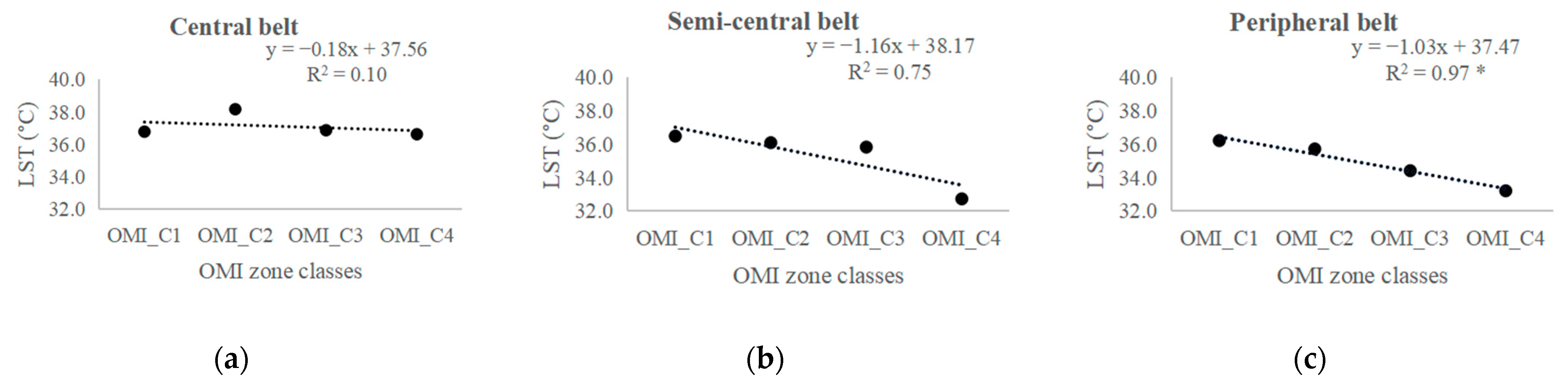
| Summer mean LST °C (95% C.I.) | 37.1 (37.1–37.1) | 35.3 (35.3–35.3) | 35.1 (35.1–35.1) | 35.4 (35.3–35.4) |
| Summer mean ALB Adim. (95% C.I.) | 0.240 (0.240–0.241) | 0.227 (0.226–0.227) | 0.228 (0.228–0.229) | 0.249 (0.247–0.250) |
| Mean SVF Adim. (95% C.I.) | 0.576 (0.576–0.577) | 0.583 (0.583–0.584) | 0.639 (0.638–0.640) | 0.746 (0.743–0.750) |
| OMI Belt | OMI Zone Classes (OMI_C) | Residential Buildings’ Real Estate Values (euro/m2) | Residential Buildings’ Number (%) | Residential Buildings in Hot-Spot Zones | Residential Buildings in Cool-Spot Zones | ||
|---|---|---|---|---|---|---|---|
| (%) | OR | (%) | OR | ||||
| Central | OMI_C1 | 3175 | 8.0 | 1.2 [4.5] | 0.20 (0.19–0.22) * | 0 [0] | - |
| OMI_C2 | 3175–3425 | 4.7 | 4.1 [15.5] | 19.40 (17.47–21.55) * | 0 [0] | - | |
| OMI_C3 | 3425–3550 | 9.0 | 2.3 [8.6] | 0.46 (0.43–0.49) * | 0 [0] | - | |
| OMI_C4 | 3550–4100 | 4.8 | 2.2 [8.2] | 1.53 (1.42–1.64) * | <0.1 [<0.1] | - | |
| Semi-central | OMI_C1 | 2375–2700 | 10.5 | 1.4 [3.2] | 9.35 (8.28–10.56) * | <0.1 [<0.1] | 0.04 (0.01–0.15) * |
| OMI_C2 | 2700–2750 | 8.0 | 0.2 [0.4] | 0.45 (0.37–0.54) * | 0 [0] | - | |
| OMI_C3 | 2750–3400 | 12.5 | 0.3 [0.8] | 0.50 (0.43–0.57) * | <0.1 [<0.1] | 0.20 (0.11–0.35) * | |
| OMI_C4 | 3400–3650 | 11.7 | 0 [0] | - | 0.2 [0.7] | 27.96 (16.15–48.40) * | |
| Peripheral | OMI_C1 | 1975–2300 | 7.6 | 0.6 [2.2] | 2.71 (2.38–3.08) * | 0 [0] | - |
| OMI_C2 | 2300–2450 | 7.1 | 0.4 [1.4] | 1.36 (1.18–1.56) * | <0.1 [<0.1] | 0.08 (0.03–0.17) * | |
| OMI_C3 | 2450–2750 | 7.6 | 0.3 [1.0] | 0.77 (0.66–0.89) * | 0.1 [0.5] | 2.41 (1.86–3.11) * | |
| OMI_C4 | 2750–3400 | 6.6 | <0.1 [<0.1] | 0.01 (0.00–0.03) * | 0.2 [0.6] | 3.66 (2.84–4.73) * | |
| Total | 100 | 13.0 | 0.6 | ||||
| Central Belt | ||||||
|---|---|---|---|---|---|---|
| Surface Thermal Zones | OMI Zone Classes (OMI_C) | Frequencies of Urban Features Mean ± Standard Deviation | ||||
| LST (°C) | IA (%) | TC (%) | GA (%) | WB (%) | ||
| Neutral | OMI_C1 | 36.6 a ± 0.7 | 93.6 a ± 7.4 | 2.4 a ± 3.9 | 3.9 a ± 4.6 | 0.1 a ± 0.6 |
| OMI_C2 | 37.1 b ± 0.6 | 93.7 b ± 8.5 | 3.0 b ± 4.0 | 3.3 b ± 5.1 | <0.1 a ± 0.5 | |
| OMI_C3 | 36.5 c ± 1.1 | 90.7 c ± 11.5 | 4.4 b ± 7.2 | 4.5 a ± 5.7 | 0.4 b ± 2.6 | |
| OMI_C4 | 35.4 d ± 1.6 | 85.6 d ± 17.8 | 6.3 b ± 10.4 | 5.8 a ± 8.7 | 2.4 c ± 6.7 | |
| p-value | <0.001 | <0.001 | <0.001 | <0.001 | <0.001 | |
| Hot-spot | OMI_C1 | 38.0 a ± 0.3 | 99.2 a ± 1.7 | 0.3 a ± 0.7 | 0.5 a ± 1.5 | - |
| OMI_C2 | 38.3 b ± 0.3 | 99.4 b ± 1.8 | 0.2 b ± 0.9 | 0.4 b ± 1.2 | - | |
| OMI_C3 | 37.9 c ± 0.2 | 99.1 a ± 1.9 | 0.4 a ± 1.3 | 0.5 c ± 1.1 | - | |
| OMI_C4 | 38.2 d ± 0.3 | 99.9 c ± 0.7 | <0.1 c ± 0.2 | 0.1 d ± 0.5 | - | |
| p-value | <0.001 | <0.001 | <0.001 | <0.001 | - | |
| Cool-spot | OMI_C1 | - | - | - | - | - |
| OMI_C2 | - | - | - | - | - | |
| OMI_C3 | - | - | - | - | - | |
| OMI_C4 | 30.1 ± 0.8 | 34.2 ± 22.7 | 47.0 ± 29.4 | 13.8 ± 9.3 | 5.0 ± 4.3 | |
| p-value | - | - | - | - | - | |
| Semi-Central Belt | ||||||
|---|---|---|---|---|---|---|
| Surface Thermal Zones | OMI Zone Classes (OMI_C) | Frequencies of Urban Features Mean ± Standard Deviation | ||||
| LST (°C) | IA (%) | TC (%) | GA (%) | WB (%) | ||
| Neutral | OMI_C1 | 36.3 a ± 1.2 | 88.9 a ± 14.0 | 4.0 a ± 7.2 | 7.0 a ± 8.6 | 0.1 a ± 1.1 |
| OMI_C2 | 36.1 b ± 1.0 | 89.3 a ± 13.0 | 3.5 a ± 5.8 | 7.0 b ± 9.1 | 0.2 b ± 1.9 | |
| OMI_C3 | 35.8 c ± 1.2 | 87.8 b ± 14.6 | 4.6 b ± 7.6 | 7.4 c ± 9.2 | 0.1 c ± 0.8 | |
| OMI_C4 | 32.8 d ± 1.6 | 49.3 c ± 23.8 | 27.9 c ± 18.4 | 22.7 d ± 14.3 | <0.1 d ± 0.3 | |
| p-value | <0.001 | <0.001 | <0.001 | <0.001 | <0.001 | |
| Hot-spot | OMI_C1 | 38.0 a ± 0.3 | 98.6 a ± 2.6 | 0.2 a ± 0.8 | 1.2 a ± 2.2 | - |
| OMI_C2 | 37.8 b ± 0.2 | 98.8 b ± 2.9 | 0.3 a ± 1.0 | 0.9 b ± 2.2 | - | |
| OMI_C3 | 38.0 a ± 0.4 | 98.9 b ± 3.5 | 0.2 a ± 1.0 | 0.9 b ± 3.0 | - | |
| OMI_C4 | - | - | - | - | - | |
| p-value | <0.001 | <0.001 | 0.370 | <0.001 | - | |
| Cool-spot | OMI_C1 | 29.7 a ± 0.8 | 25.3 a ± 1.2 | 57.6 a ± 2.2 | 17.0 a,b ± 1.0 | - |
| OMI_C2 | - | - | - | - | - | |
| OMI_C3 | 29.6 a ± 0.5 | 45.7 b ± 5.7 | 33.7 b ± 8.0 | 20.7 a ± 7.8 | - | |
| OMI_C4 | 29.6 a ± 0.6 | 24.1 a ± 10.4 | 61.1 a ± 12.7 | 14.7 b ± 7.9 | 0.1 ± 0.7 | |
| p-value | 0.974 | <0.001 | <0.001 | 0.046 | - | |
| Peripheral Belt | ||||||
|---|---|---|---|---|---|---|
| Surface Thermal Zones | OMI zone Classes (OMI_C) | Frequencies of Urban Features Mean ± Standard Deviation | ||||
| LST (°C) | IA (%) | TC (%) | GA (%) | WB (%) | ||
| Neutral | OMI_C1 | 36.1 a ± 1.0 | 82.0 a ± 15.7 | 4.8 a ± 7.4 | 13.2 a ± 11.9 | 0.0 c ± 0.5 |
| OMI_C2 | 35.6 b ± 1.5 | 72.9 b ± 21.9 | 8.3 b ± 11.5 | 18.6 b ± 15.0 | 0.2 a ± 1.9 | |
| OMI_C3 | 34.4 c ± 2.1 | 62.4 c ± 28.4 | 14.9 c ± 16.8 | 22.6 c ± 18.2 | 0.2 b ± 1.2 | |
| OMI_C4 | 33.3 d ± 1.8 | 55.4 d ± 25.8 | 20.4 d ± 16.2 | 24.0 d ± 17.2 | 0.2 a,b ± 1.2 | |
| p-value | <0.001 | <0.001 | <0.001 | <0.001 | <0.001 | |
| Hot-spot | OMI_C1 | 37.8 a ± 0.2 | 96.5 a ± 5.1 | 0.5 a ± 1.3 | 3.0 a ± 4.6 | - |
| OMI_C2 | 38.1 b ± 0.6 | 94.6 b ± 7.8 | 0.6 b ± 2.0 | 4.8 b ± 6.6 | - | |
| OMI_C3 | 38.0 b ± 0.4 | 95.8 a,b ± 6.5 | 0.3 a,b ± 0.9 | 3.9 a,b ± 6.2 | - | |
| OMI_C4 | 37.3 c ± 0.0 | 86.6 b ± 8.7 | 4.8 c ± 3.9 | 6.4 a,b ± 3.0 | 2.2 ± 1.8 | |
| p-value | <0.001 | 0.043 | <0.001 | 0.015 | - | |
| Cool-spot | OMI_C1 | - | - | - | - | - |
| OMI_C2 | 29.5 a ± 1.5 | 26.9 a ± 12.3 | 56.0 a ± 18.4 | 16.9 a ± 16.1 | 0.3 a ± 0.8 | |
| OMI_C3 | 29.2 a ± 0.8 | 21.1 a ± 9.4 | 59.5 a ± 13.1 | 19.1 a ± 11.3 | 0.3 a ± 1.2 | |
| OMI_C4 | 29.1 a ± 0.7 | 23.7 a ± 9.2 | 57.4 a ± 13.0 | 18.4 a ± 8.4 | 0.5 a ± 2.3 | |
| p-value | 0.261 | 0.200 | 0.373 | 0.723 | 0.855 | |
Publisher’s Note: MDPI stays neutral with regard to jurisdictional claims in published maps and institutional affiliations. |
© 2022 by the authors. Licensee MDPI, Basel, Switzerland. This article is an open access article distributed under the terms and conditions of the Creative Commons Attribution (CC BY) license (https://creativecommons.org/licenses/by/4.0/).
Share and Cite
Guerri, G.; Crisci, A.; Cresci, I.; Congedo, L.; Munafò, M.; Morabito, M. Residential Buildings’ Real Estate Values Linked to Summer Surface Thermal Anomaly Patterns and Urban Features: A Florence (Italy) Case Study. Sustainability 2022, 14, 8412. https://doi.org/10.3390/su14148412
Guerri G, Crisci A, Cresci I, Congedo L, Munafò M, Morabito M. Residential Buildings’ Real Estate Values Linked to Summer Surface Thermal Anomaly Patterns and Urban Features: A Florence (Italy) Case Study. Sustainability. 2022; 14(14):8412. https://doi.org/10.3390/su14148412
Chicago/Turabian StyleGuerri, Giulia, Alfonso Crisci, Irene Cresci, Luca Congedo, Michele Munafò, and Marco Morabito. 2022. "Residential Buildings’ Real Estate Values Linked to Summer Surface Thermal Anomaly Patterns and Urban Features: A Florence (Italy) Case Study" Sustainability 14, no. 14: 8412. https://doi.org/10.3390/su14148412