
Demand Response Analysis Framework (DRAF): An Open-Source Multi-Objective Decision Support Tool for Decarbonizing Local Multi-Energy Systems


Abstract
:1. Introduction
1.1. Demand Response
1.1.1. DR in the Industrial and Commercial Sector
1.1.2. DR and Investments
1.1.3. DR and Carbon Emissions
1.2. Energy System Optimization
1.2.1. Multi-Objective Mixed Integer Linear Programming
1.2.2. Open-Source
1.2.3. Other Energy System Frameworks/Models
- Model adaptation to industry-specific conditions;
- Research and processing of market data, such as dynamic CEFs (depending on the country, year, and temporal resolution) and cost functions;
- Generation of weather-dependent energy-relevant time series, such as energy yield time series for photovoltaics (PVs) or thermal load profiles;
- Preparation, analysis, and plausibility checking of project-specific data, such as electrical load profiles,
- Model parameterization;
- Adaptation of result output functions, such as plots and tables to the particular data structure.
1.3. Contributions
2. The Demand Response Analysis Framework (DRAF)
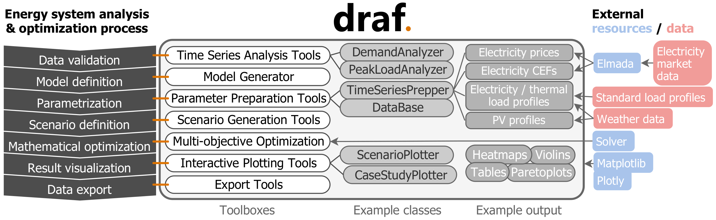
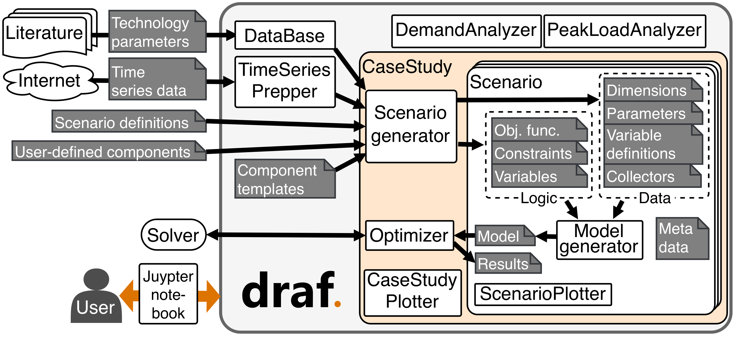
2.1. Overview
2.2. Python as a High Level Programming Language
2.3. Time Series Analysis Tools
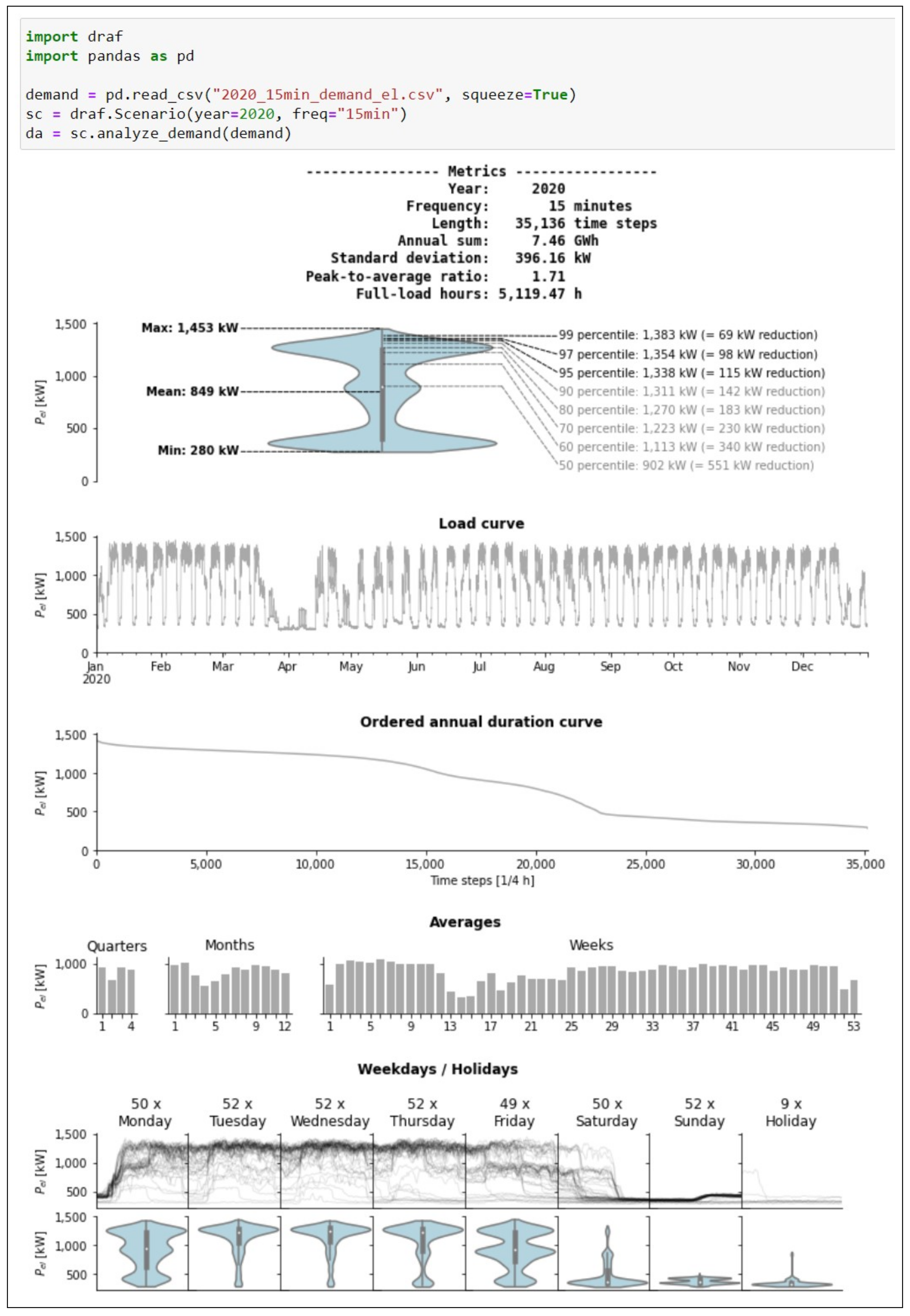
2.3.1. DemandAnalyzer
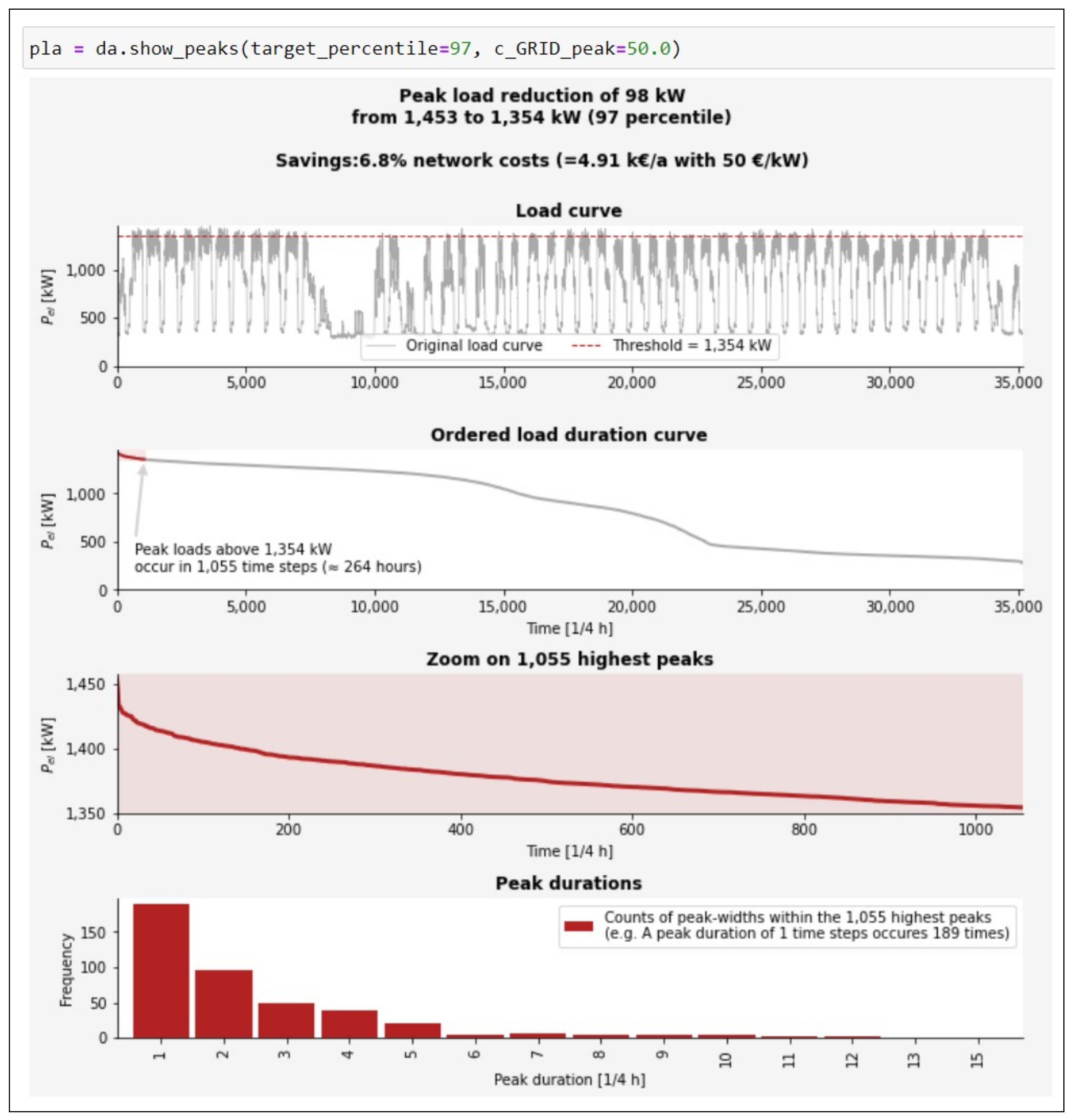
2.3.2. PeakLoadAnalyzer
2.4. Parameter Preparation Tools
2.4.1. TimeSeriesPrepper
Carbon Emission Factors (CEFs) and Electricity Prices
Photovoltaic Power Profiles
Electrical and Thermal Load Profiles
2.4.2. DataBase
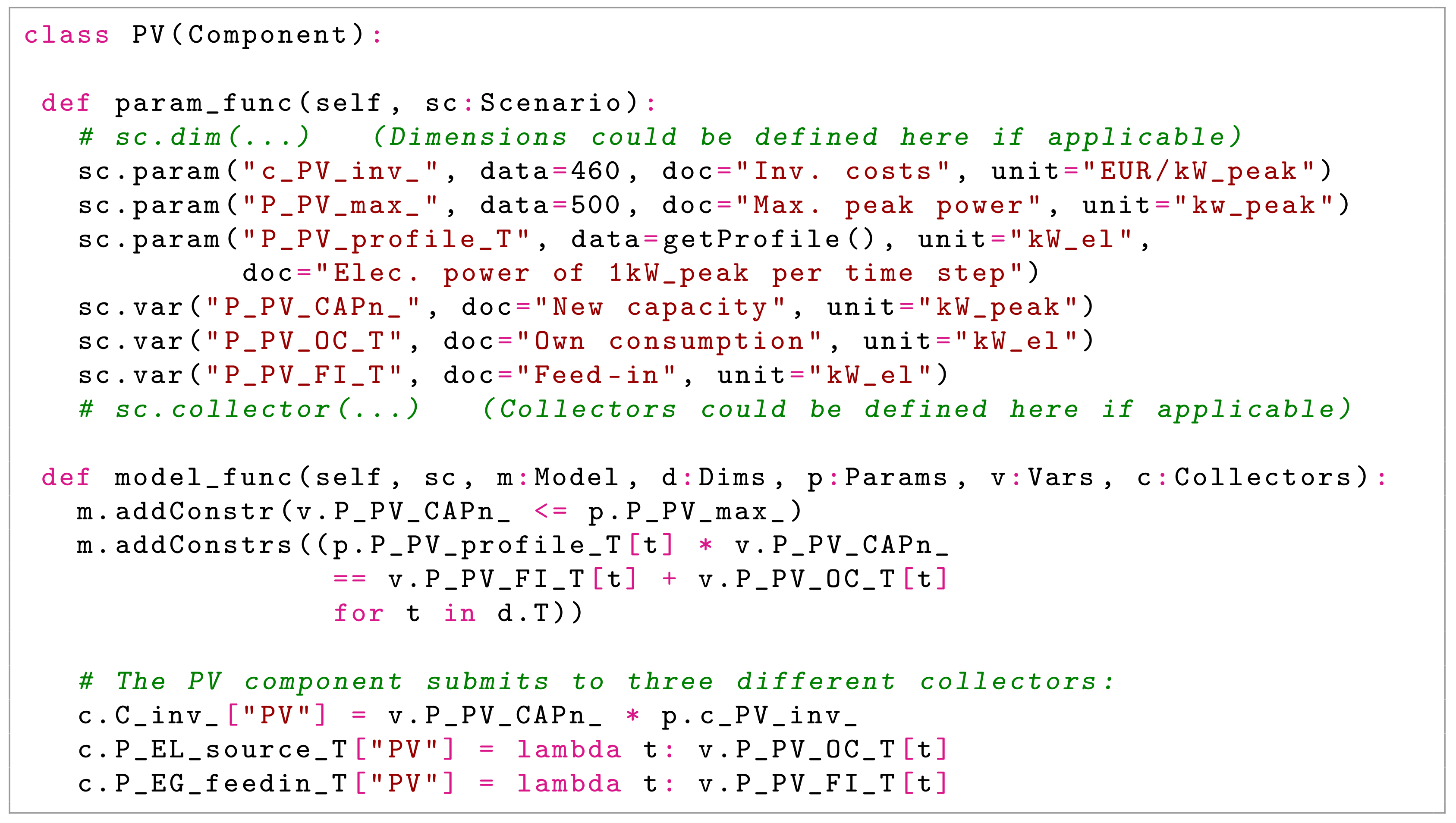
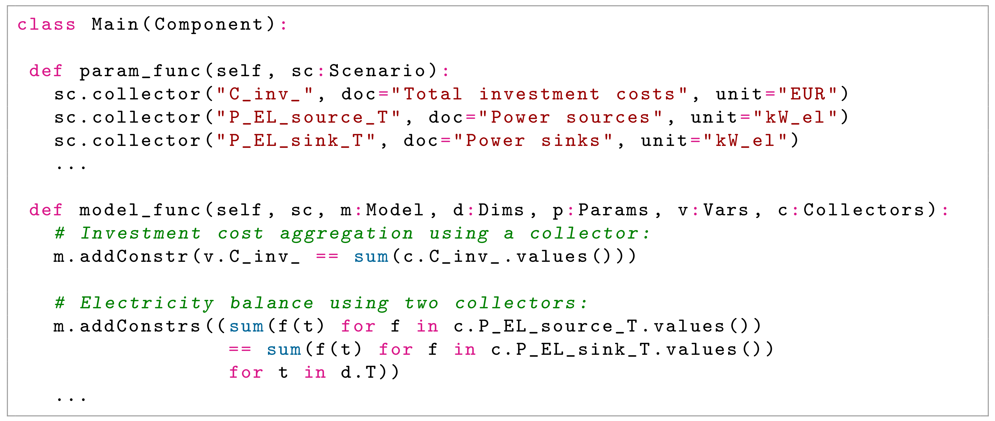
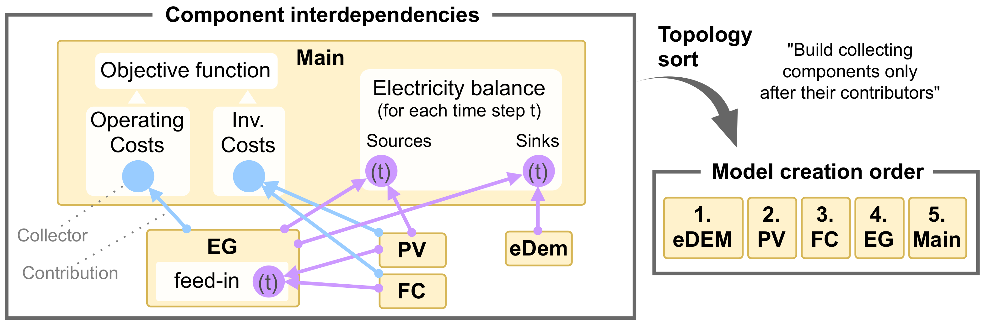
2.5. Component-Based Model Generator
| Algorithm 1: Model generation. |
 |
2.6. Component Templates
2.6.1. The Component Template Main
2.6.2. Technology Component Templates
2.7. Scenario Generation and Optimization
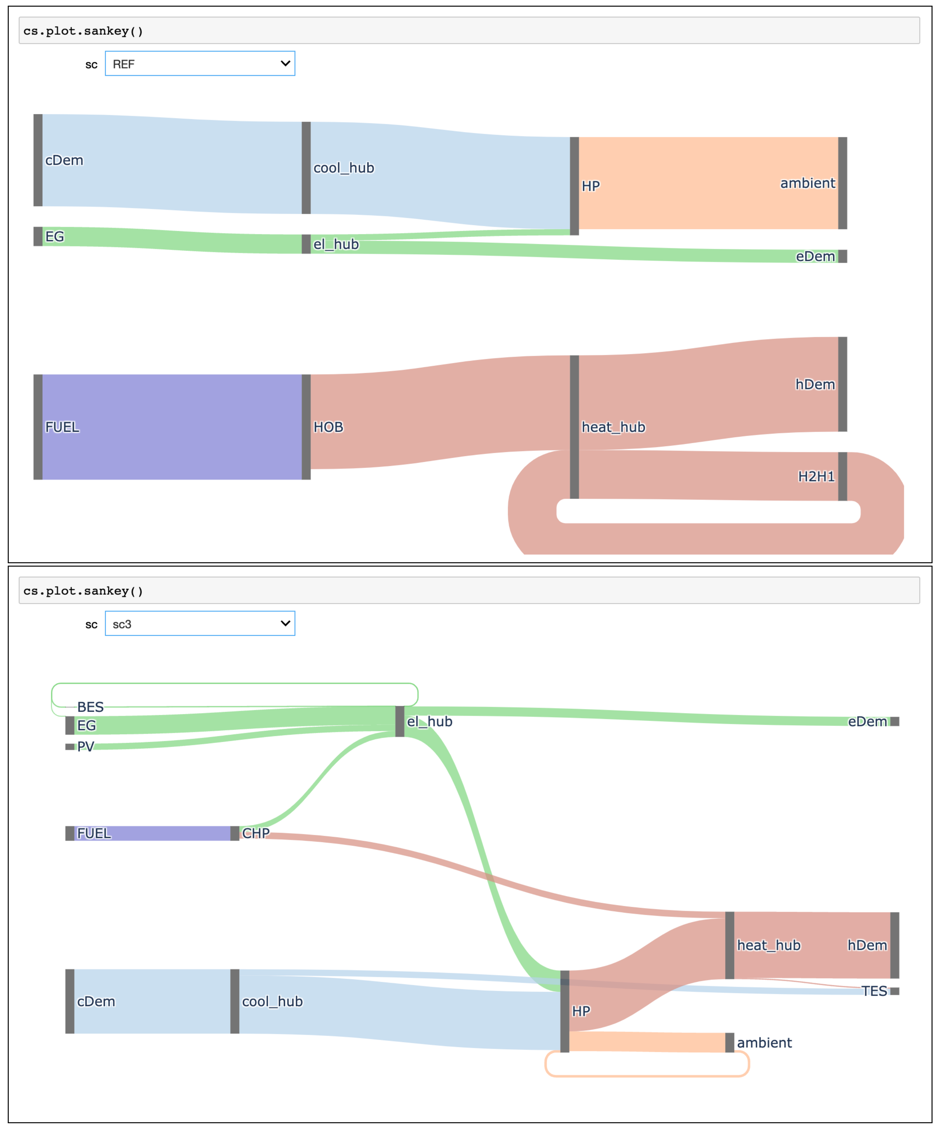
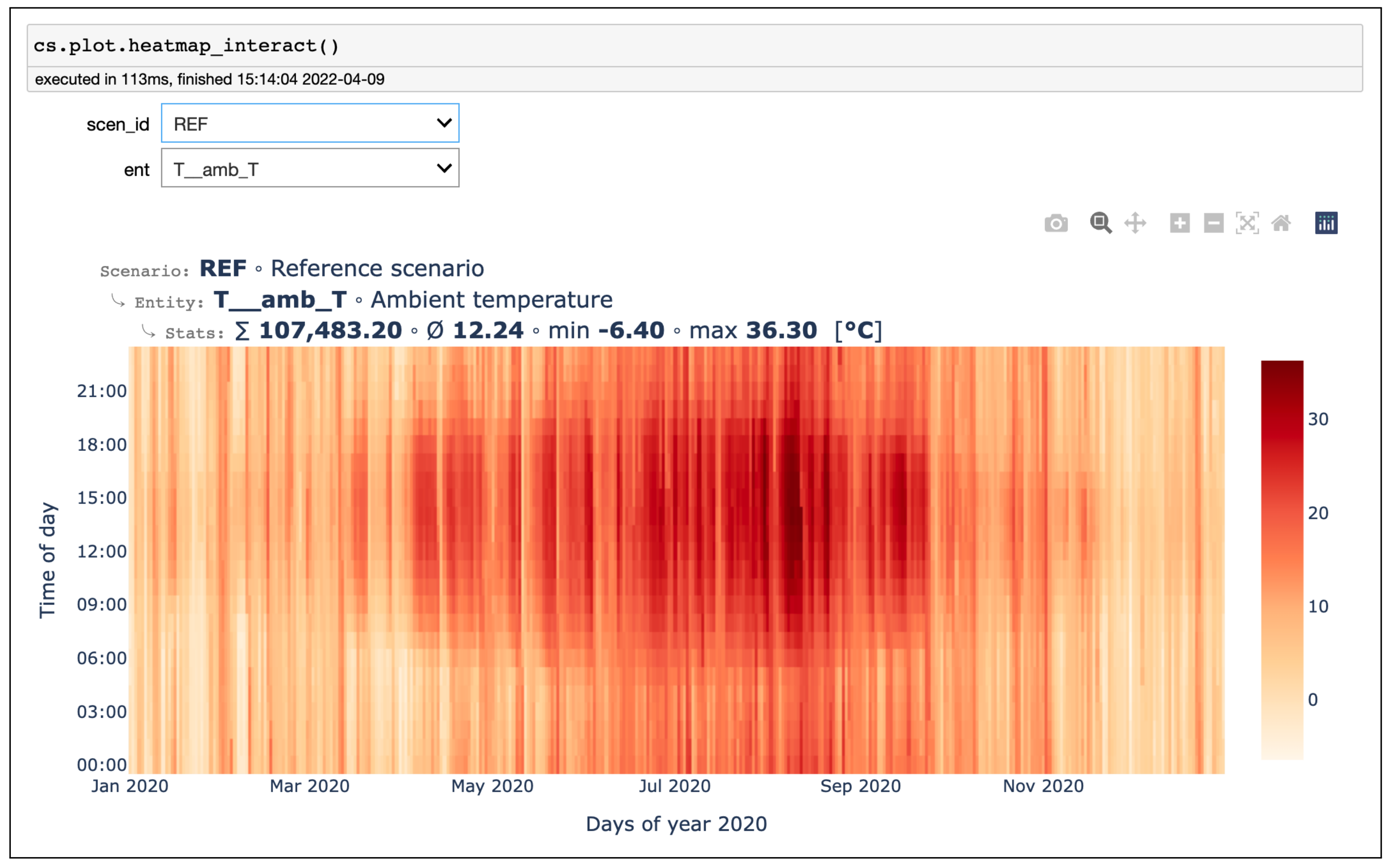
2.8. Visualization
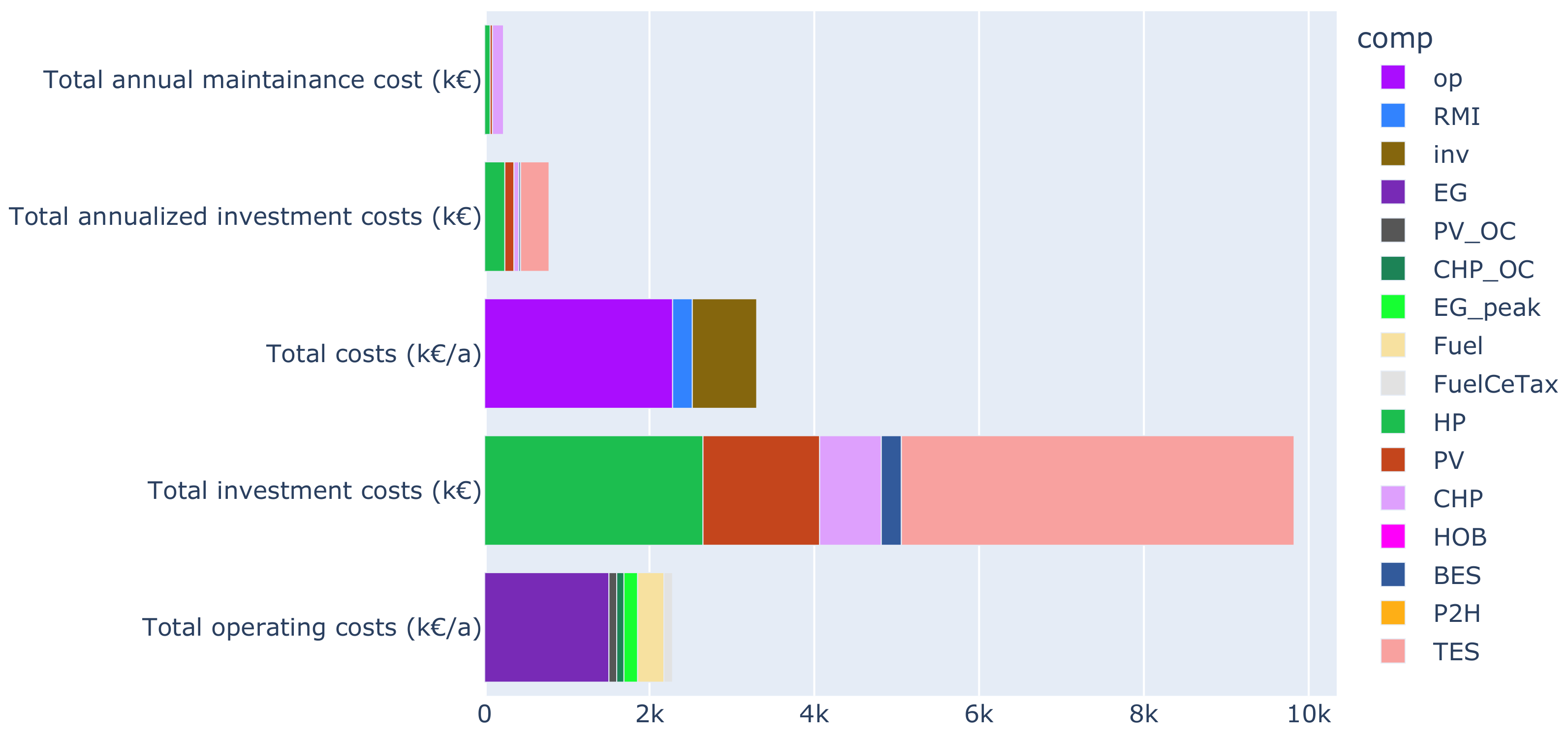
3. Case Studies
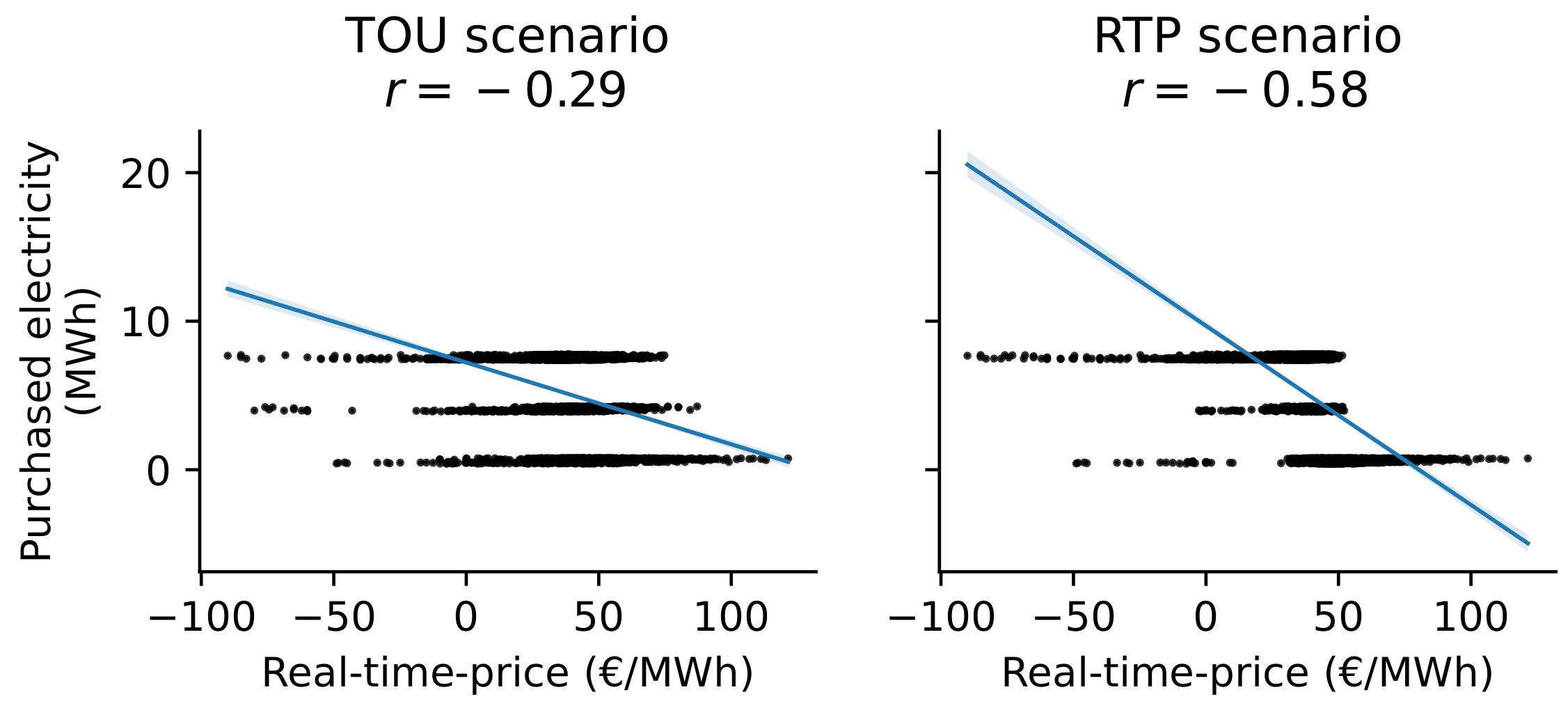
3.1. Case Study 1: Price-Based DR Potential of an Industrial Production Process
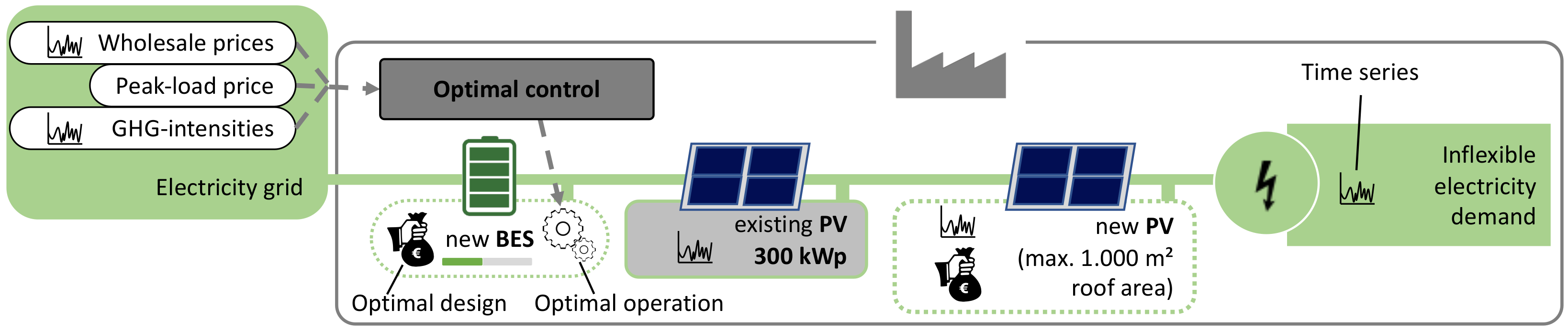
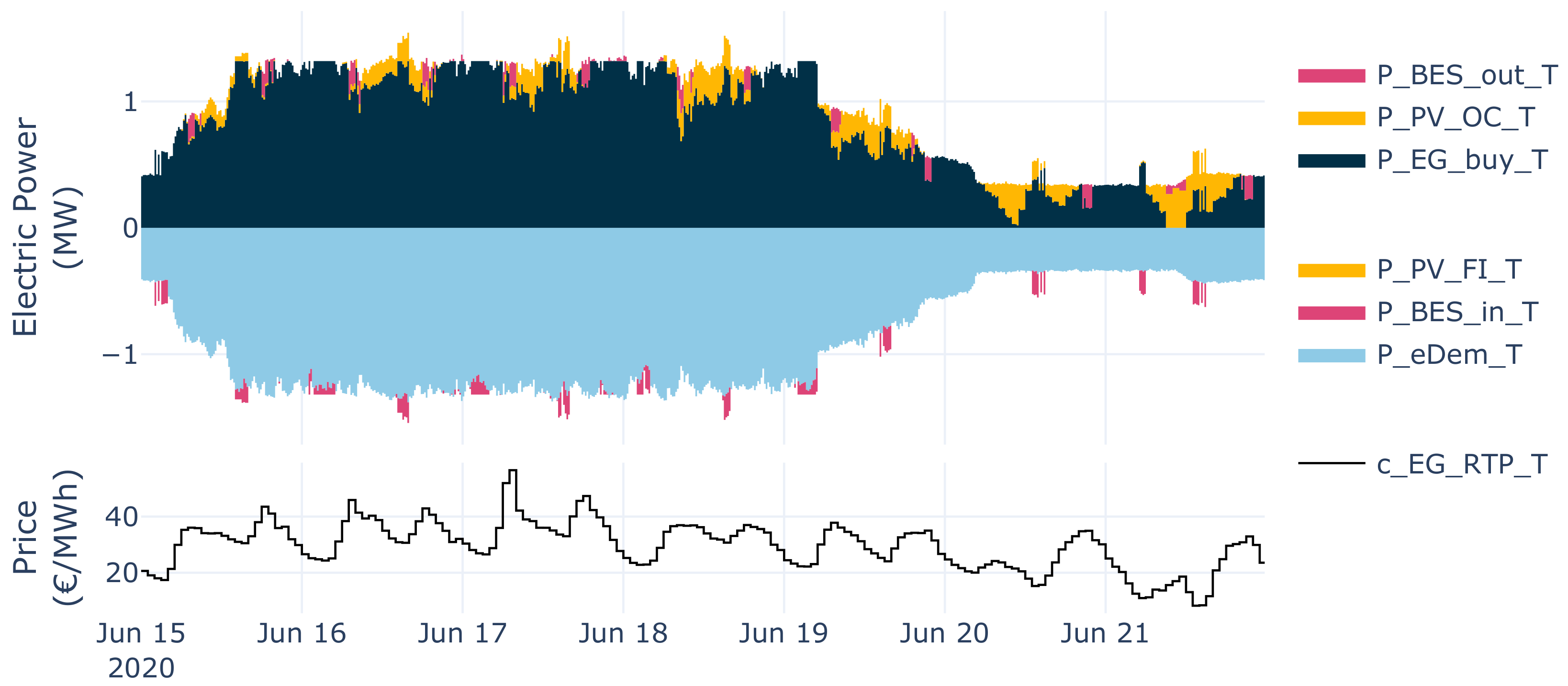
3.2. Case Study 2: Design Optimization of a Multi-Use BES and PV System
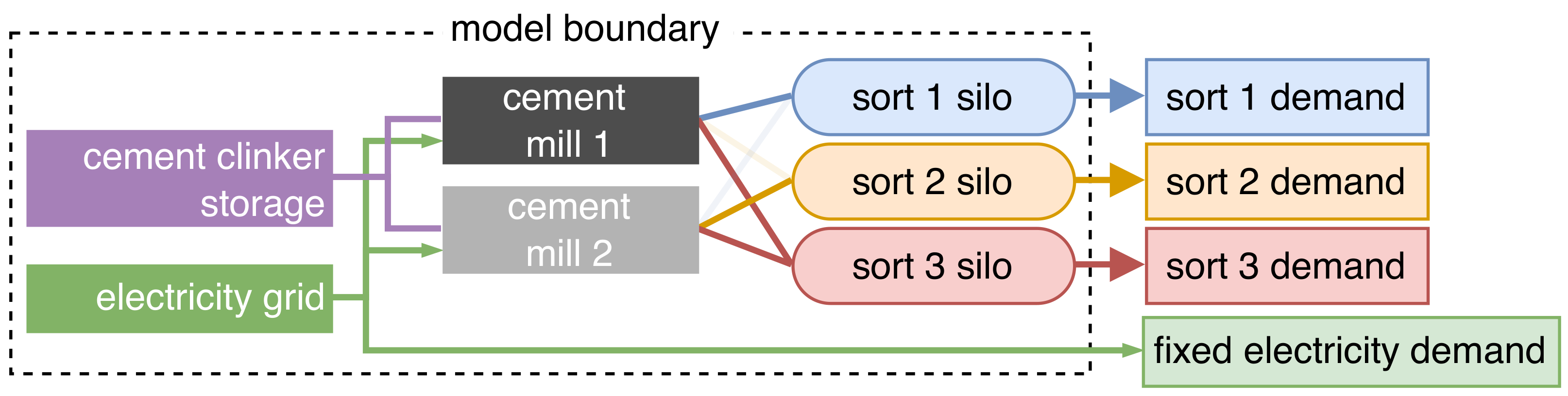
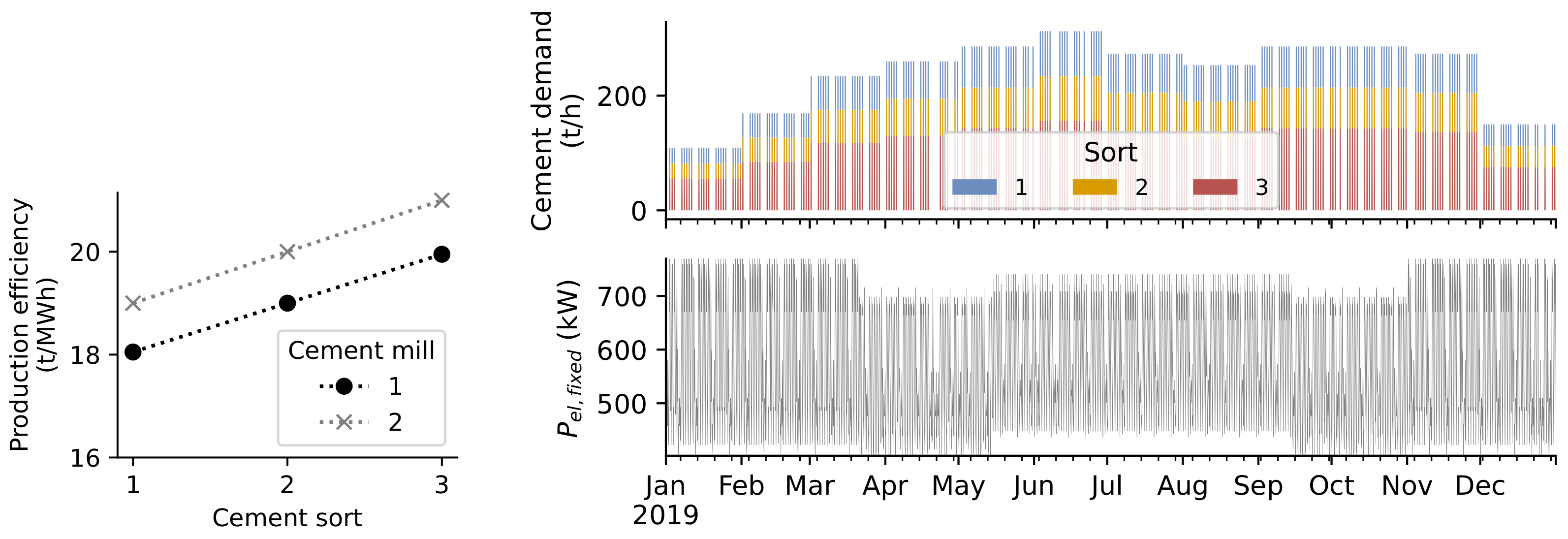
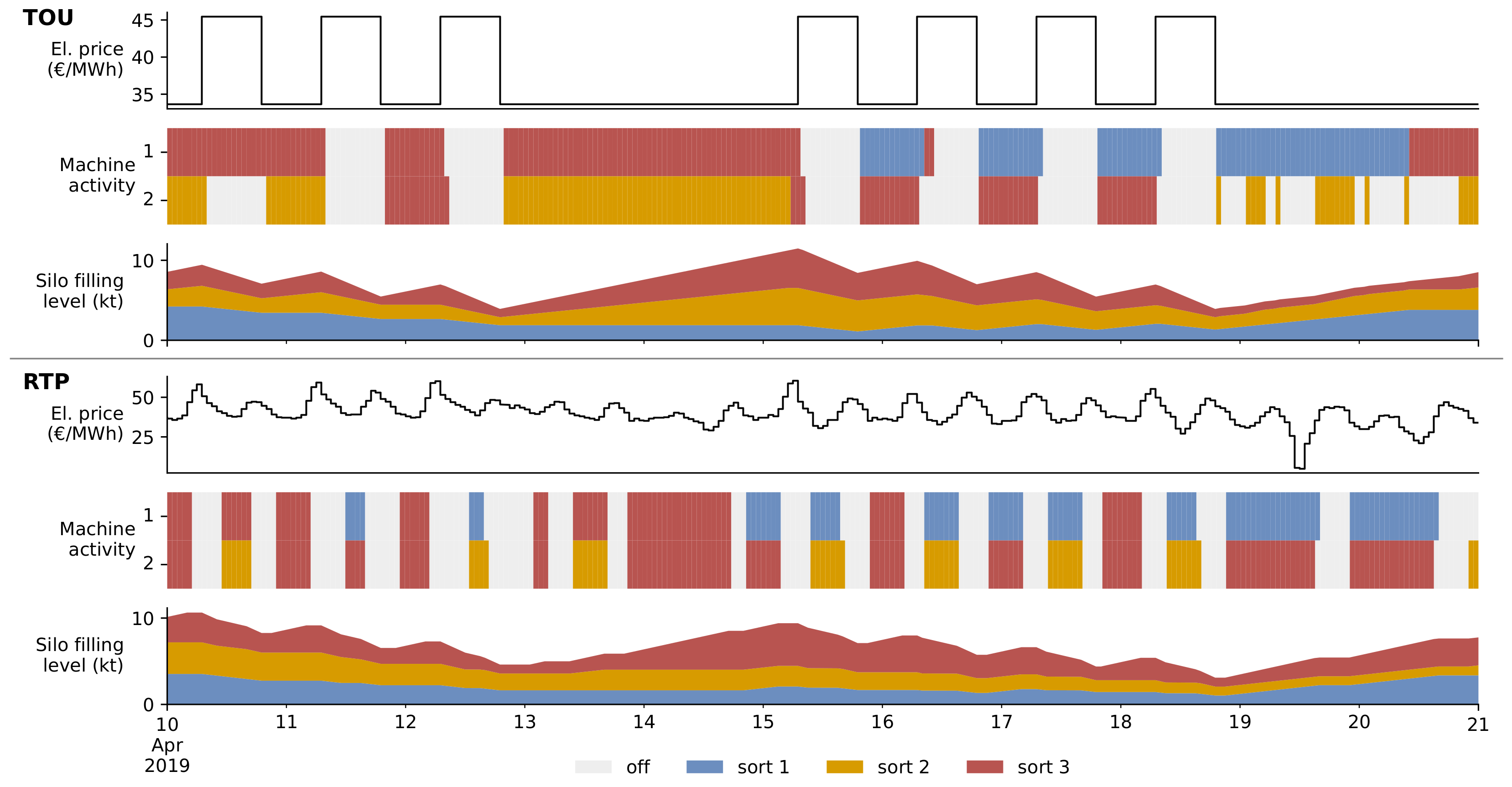
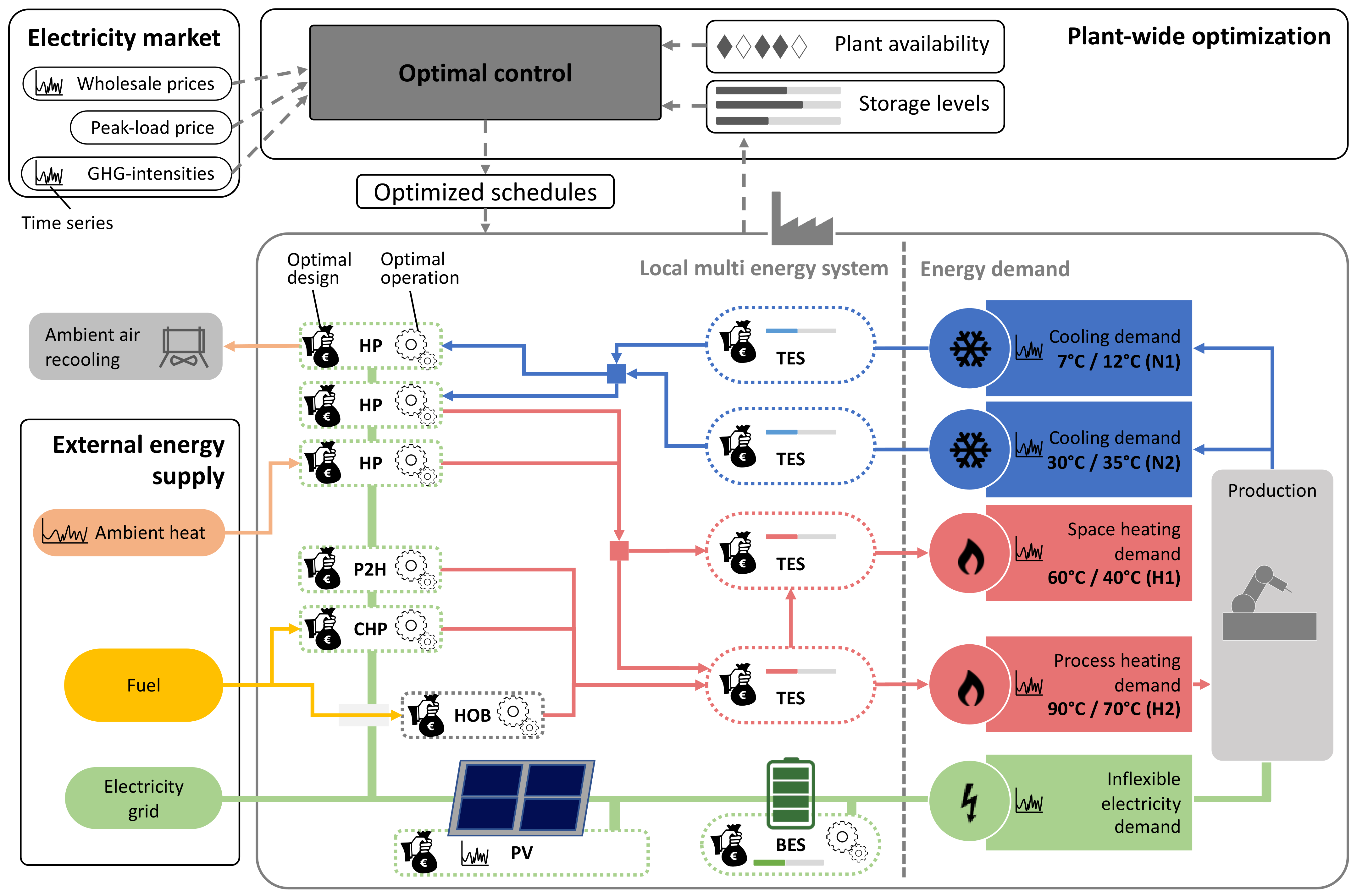
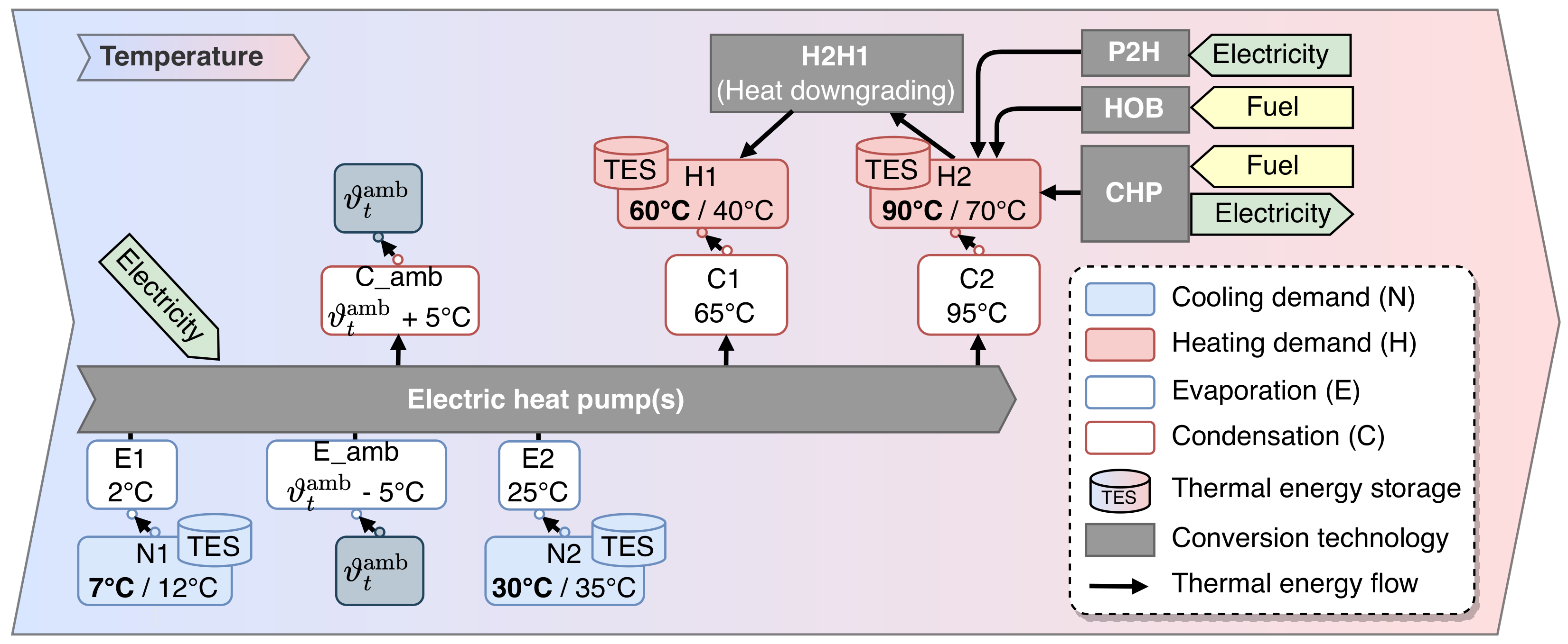
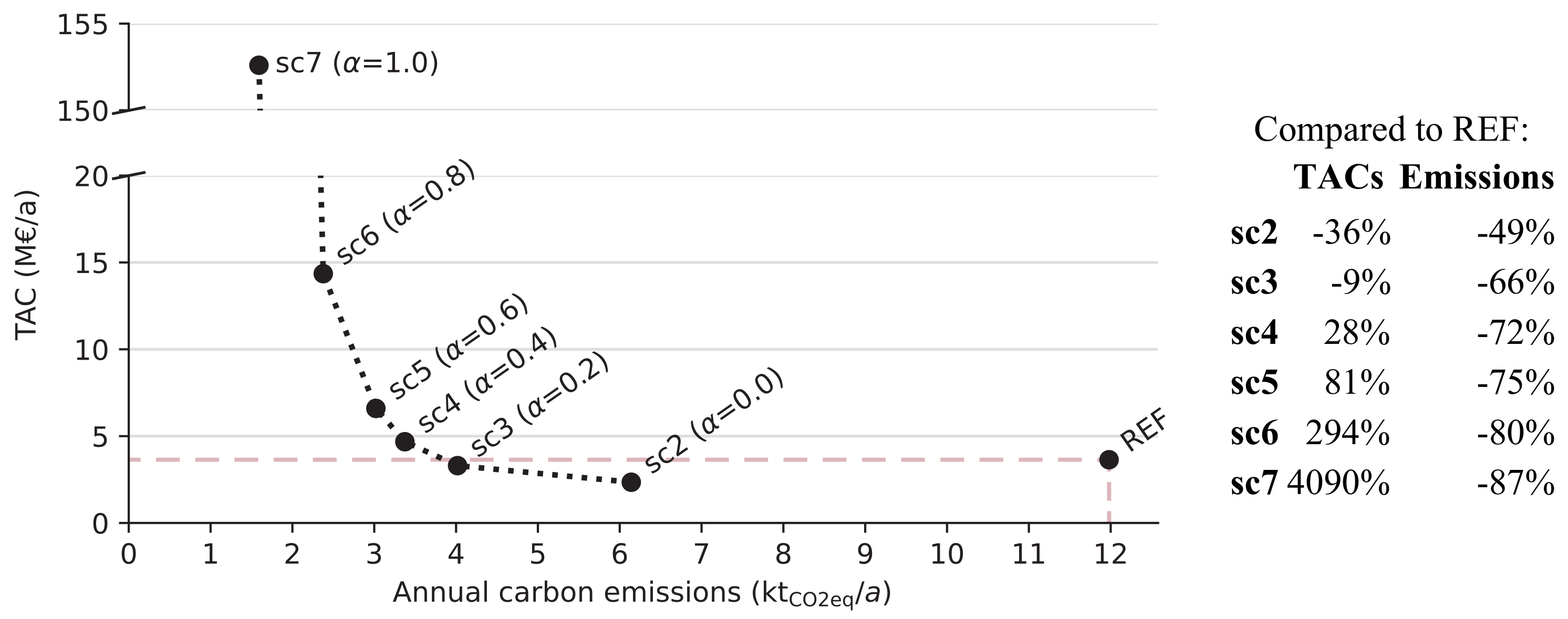
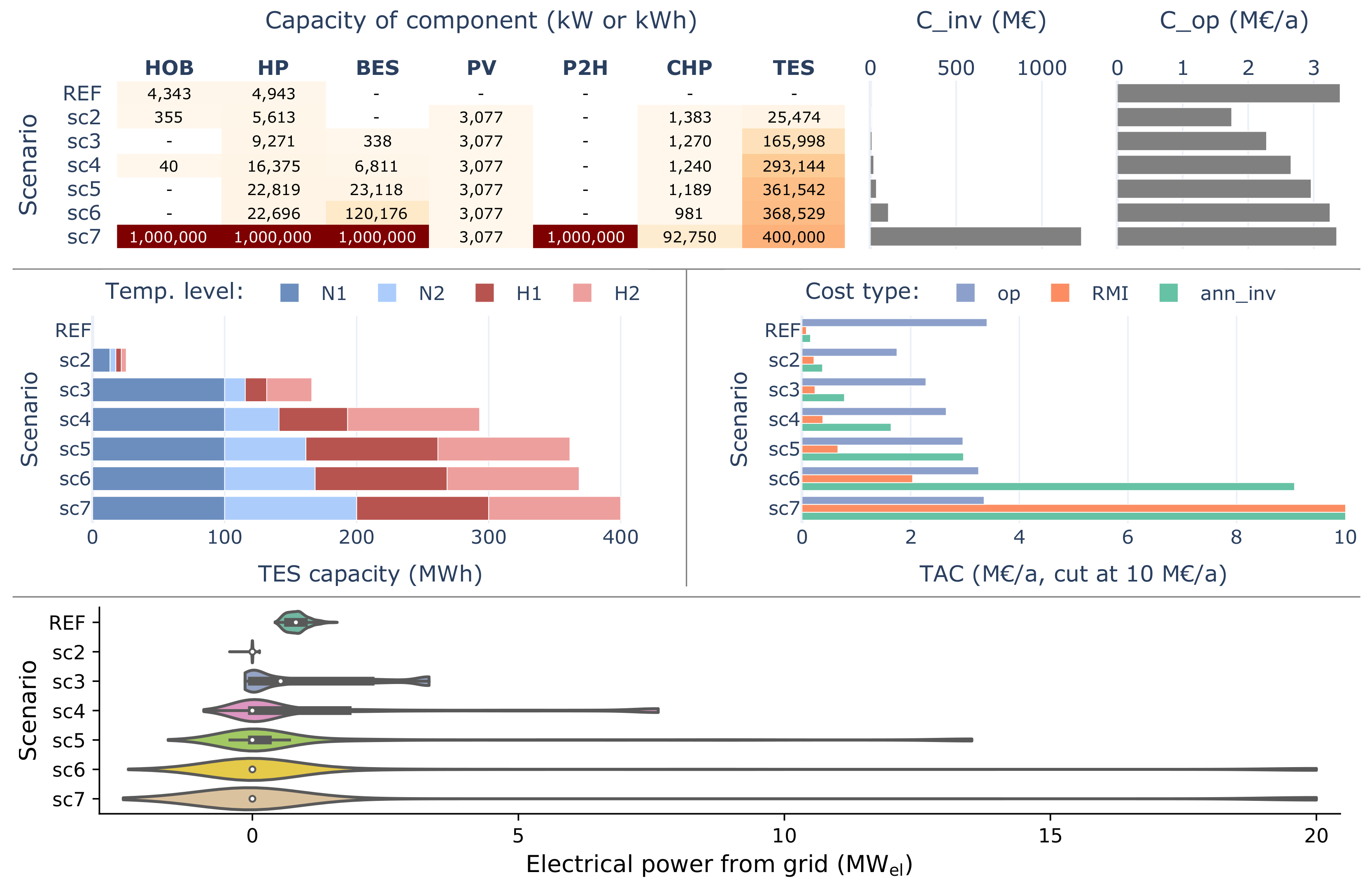
3.3. Case Study 3: Multi-Objective Design and Operational Optimization of Thermal-Electric Sector Coupling
4. Conclusions
Author Contributions
Funding
Institutional Review Board Statement
Informed Consent Statement
Data Availability Statement
Conflicts of Interest
Nomenclature
| Acronyms | |
| CEF | Carbon emission factor |
| COP | Coefficient of performance |
| DR | Demand response |
| DRAF | Demand response analysis framework |
| HP | Electric heat pump |
| L-MES | Local multi-energy system |
| MEF | Marginal emission factor |
| MILP | Mixed-integer linear programming |
| PBDR | Price-based demand response |
| RES | Renewable energy sources |
| RTP | Real-time prices |
| TAC | Total annualized cost |
| TOU | Time of use |
| XEF | Grid mix emission factor |
| Component Labels | |
| bes | Battery energy storage |
| bev | Battery electric vehicle |
| cdem | Cooling demand |
| chp | Combined heat and power |
| edem | Electricity demand |
| eg | Electricity grid |
| fuel | Fuels |
| h2h | Heat downgrading |
| hdem | Heat demand |
| hob | Heat-only boiler |
| hp | Electric heat pumps |
| p2h | Power-to-heat |
| pp | Production process |
| ps | Product storage |
| pv | Photovoltaic system |
| tes | Thermal energy storage |
| Symbols | |
| A | Area |
| C | Costs |
| c | Specific costs |
| CE | Carbon emissions |
| ce | Specific carbon emissions |
| cop | Coefficient of performance |
| Product flow | |
| Time step | |
| Heat flow | |
| E | Electrical energy |
| Efficiency | |
| F | Fuel flow |
| G | Product |
| k | A ratio |
| n | A natural number |
| N | Operation life |
| P | Electrical power |
| Q | Thermal energy |
| T | Temperature |
| y | Binary indicator |
| Superscripts | |
| capn | New capacity |
| capx | Existing capacity |
| cond | Condensation |
| eva | Evaporation |
| fi | Feed-in |
| minpl | Minimal part load |
| oc | Own consumption |
| rmi | Repair, maintenance, and inspection |
| Indices and Sets | |
| Condensation temperature levels | |
| Fuel types | |
| Heating temperature levels | |
| Flow types | |
| Technology components | |
| Thermal demand temperature levels | |
| Cooling temperature levels | |
| Time steps | |
Appendix A. Screenshots of DRAF Output
Appendix A.1. DemandAnalyzer

Appendix A.2. PeakLoadAnalyzer

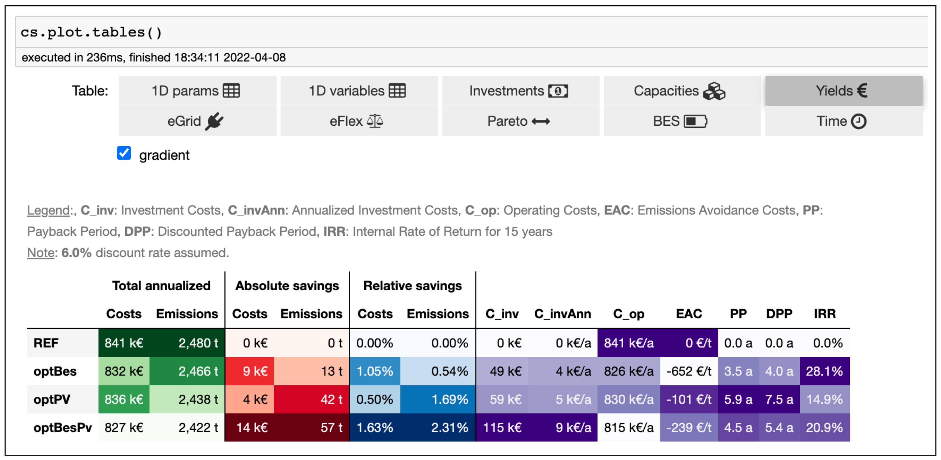
Appendix A.3. Result Visualization


Appendix B. Component Templates Definitions

Appendix B.1. Electricity Grid (EG)
| Symbol | Default | Src | Unit | Description |
| - | kgCO2eq/kWhel | Carbon emission factors (via elmada using year, freq, country, and CEF-method) | ||
| 0.131 | €/kWhel | Electricity taxes and levies | ||
| 50.000 | €/kWel/a | Peak price | ||
| - | €/kWhel | Flat-electricity tariff (calculated from Real-time-price) | ||
| - | €/kWhel | Day-ahead-market-prices (via elmada using year, freq, and country) | ||
| - | €/kWhel | Time-Of-Use-tariff (calculated from Real-time-price) | ||
| - | €/kWhel | Chosen electricity tariff | ||
| - | kWel | Peak electrical power | ||
| - | kWel | Purchased electrical power | ||
| - | kWel | Selling electrical power |
Appendix B.2. Fuels (Fuel)
| Symbol | Default | Src | Unit | Description |
| - | kW | Total fuel consumption |
Appendix B.3. Battery Energy Storage (BES)
| Symbol | Default | Src | Unit | Description |
| 0.000 | kWhel | Existing capacity | ||
| 20.000 | [84] | a | Operation life | |
| 97.468 | [85] | % | Charging efficiency | |
| 97.468 | [85] | % | Discharging efficiency | |
| 99.998 | [86] | %/h | Efficiency due to self-discharge rate | |
| 720.000 | [87] | €/kWhel | CAPEX | |
| 0.000 | % | Initial and final energy filling share | ||
| 70.000 | [88] | % | Maximum charging power per capacity | |
| 70.000 | [88] | % | Maximum discharging power per capacity | |
| 2.000 | [84] | % | Repair, maintenance, and inspection per year and investment cost | |
| - | kWhel | New capacity | ||
| - | kWhel | Electricity stored | ||
| - | kWel | Charging power | ||
| - | kWel | Discharging power |
Appendix B.4. Thermal Energy Storage (TES)
| Symbol | Default | Src | Unit | Description |
| 30.000 | [78] | a | Operation life | |
| - | kWhth | Existing capacity | ||
| 99.500 | % | Storing efficiency | ||
| 28.709 | [91] | €/kWth | CAPEX | |
| - | % | Initial and final energy level share | ||
| 50.000 | % | Ratio loading power/capacity | ||
| 50.000 | % | Ratio loading power/capacity | ||
| 0.100 | [91] | % | Repair, maintenance, and inspection per year and investment cost | |
| - | kWhth | New capacity | ||
| - | kWhth | Stored heat | ||
| - | kWth | Storage input heat flow |
Appendix B.5. Photovoltaic System (PV)
| Symbol | Default | Src | Unit | Description |
| 100.000 | m2 | Area available for new PV | ||
| 6.500 | m2/kWpeak | Area efficiency of new PV | ||
| 25.000 | [92] | a | Operation life | |
| 0.000 | kWpeak | Existing capacity | ||
| - | [72] | kWel/kWpeak | Produced PV-power for 1 kWpeak | |
| 460.000 | [83] | €/kWpeak | CAPEX | |
| 0.028 | [93] | €/kWhel | Renewable Energy Law (EEG) levy on own consumption | |
| 2.000 | [92] | % | Repair, maintenance, and inspection per year and investment cost | |
| - | kWpeak | New capacity | ||
| - | kWel | Feed-in | ||
| - | kWel | Own consumption |
Appendix B.6. Battery Electric Vehicle (BEV)
| Symbol | Default | Src | Unit | Description |
| - | kWhel | Capacity of one battery | ||
| - | kWhel | Capacity of all batteries | ||
| - | kWel | Power use | ||
| 97.468 | [85] | % | Charging efficiency | |
| 97.468 | [85] | % | Discharging efficiency | |
| 100.000 | % | Storing efficiency. Must be 1.0 for the uncontrolled charging in REF | ||
| - | % | Minimum state of charge | ||
| - | % | Maximum state of charge | ||
| - | % | Initial and final state of charge | ||
| - | [88] | % | Maximum charging power per capacity | |
| - | [88] | % | Maximum v2x discharging power per capacity | |
| - | - | Number of batteries | ||
| - | - | If BEV is available for charging at time step | ||
| 0.000 | - | If smart charging is allowed | ||
| 0.000 | - | If vehicle-to-X is allowed | ||
| - | kWhel | Electricity stored in BEV battery | ||
| - | kWel | Charging power | ||
| - | kWel | Discharging power for vehicle-to-X | ||
| - | - | Penalty to ensure uncontrolled charging in REF |
Appendix B.7. Combined Heat and Power (CHP)
| Symbol | Default | Src | Unit | Description |
| 25.000 | [94] | a | Operation life | |
| 0.000 | kWel | Existing capacity | ||
| 100,000.000 | kWel | Big-M number (upper bound for CAPn + CAPx) | ||
| 40.000 | [95] | % | Electric efficiency | |
| 45.000 | [95] | % | Thermal efficiency | |
| 589.458 | [96] | €/kWel | CAPEX | |
| 0.028 | [93] | €/kWhel | Renewable Energy Law (EEG) levy on own consumption | |
| 50.000 | % | Minimal allowed part load | ||
| 18.000 | [94] | % | Repair, maintenance, and inspection per year and investment cost | |
| - | kW | Consumed fuel flow | ||
| - | kWel | New capacity | ||
| - | kWel | Feed-in | ||
| - | kWel | Own consumption | ||
| - | kWel | Producing power | ||
| - | - | Binary: If in operation | ||
| - | kWth | Producing heat flow |
Appendix B.8. Heat-Only Boiler (HOB)
| Symbol | Default | Src | Unit | Description |
| 15.000 | [94] | a | Operation life | |
| 0.000 | kWth | Existing capacity | ||
| 90.000 | [94] | % | Thermal efficiency | |
| 57.133 | [97] | €/kWth | CAPEX | |
| 18.000 | [94] | % | Repair, maintenance, and inspection per year and investment cost | |
| - | kW | Input fuel flow | ||
| - | kWth | New capacity | ||
| - | kWth | Ouput heat flow |
Appendix B.9. Power-to-Heat (P2H)
| Symbol | Default | Src | Unit | Description |
| 30.000 | a | Operation life | ||
| 0.000 | kWth | Existing capacity | ||
| 90.000 | [98] | % | Efficiency | |
| 100.000 | [99] | €/kWth | System CAPEX | |
| 0.000 | % | Repair, maintenance, and inspection per year and investment cost | ||
| - | kWel | Consuming power | ||
| - | kWth | New capacity | ||
| - | kWth | Producing heat flow |
Appendix B.10. Electric Heat Pump (HP)
| Symbol | Default | Src | Unit | Description |
| 18.000 | [100] | a | Operation life | |
| 0.000 | kWth | Existing heating capacity | ||
| 100,000.000 | kWth | Big-M number (upper bound for CAPn + CAPx) | ||
| 50.000 | [101] | % | Ratio of reaching the ideal COP (exergy efficiency) | |
| - | °C | Condensation side temperature | ||
| - | °C | Evaporation side temperature | ||
| 285.788 | [102] | €/kWel | CAPEX | |
| 2.500 | [100] | % | Repair, maintenance, and inspection per year and investment cost | |
| 1.000 | - | Maximum number of parallel operation modes | ||
| - | kWel | Consuming power | ||
| - | - | Binary: If source and sink are connected at time-step | ||
| - | kWth | New heating capacity | ||
| - | kWth | Heat flow released on condensation side | ||
| - | kWth | Heat flow absorbed on evaporation side |
Appendix B.11. Heat Downgrading (H2H1)
| Symbol | Default | Src | Unit | Description |
| - | kWth | Heat down-grading |
Appendix B.12. Product Demand (pDem)
Appendix B.13. Production Process (PP)
| Symbol | Default | Src | Unit | Description |
| - | kWel | |||
| - | % | Production efficiency | ||
| 10.000 | €/change | Costs per sort change | ||
| 10.000 | €/SU | Costs per start up | ||
| - | % | Minimum part load | ||
| - | - | If machine is available at time step | ||
| - | - | If machine and sort is compatible | ||
| - | k€ | Total cost of sort change | ||
| - | k€ | Total cost of start up | ||
| - | kWel | Nominal power consumption of machine | ||
| - | - | Binary: If machine is in operation | ||
| - | - | Binary: If sort has just changed | ||
| - | - | Binary: If machine just started up | ||
| - | t/h | Production of machine |
Appendix B.14. Product Storage (PS)
| Symbol | Default | Src | Unit | Description |
| - | t | Existing storage capacity of product | ||
| 50.000 | a | Operation life | ||
| 1000.000 | €/t | Investment cost | ||
| - | % | Initial storage filling level | ||
| - | % | Share of minimal required storage filling level | ||
| - | kWhel | Energy equivalent | ||
| - | t | New capacity | ||
| - | t | Final time step deviation from init | ||
| - | t | Storage filling level |
Appendix B.15. Cooling Demand (cDem)
| Symbol | Default | Src | Unit | Description |
| - | kWth | Cooling demand | ||
| - | °C | Cooling inlet temperature | ||
| - | °C | Cooling outlet temperature |
Appendix B.16. Heating Demand (hDem)
| Symbol | Default | Src | Unit | Description |
| - | kWth | Heating demand | ||
| - | °C | Heating inlet temperature | ||
| - | °C | Heating outlet temperature |
Appendix B.17. Electricity Demand (eDem)
| Symbol | Default | Src | Unit | Description |
| - | kWel | Electricity demand from standard load profile G3: Business continuous |
References
- United Nations Framework Convention of Climate Change. Paris Agreement on Paris Climate Change Conference—November 2015. Available online: https://unfccc.int/sites/default/files/english_paris_agreement.pdf (accessed on 25 August 2021).
- United Nations Framework Convention of Climate Change. Glasgow Climate Pact—November 2021. Available online: https://unfccc.int/sites/default/files/resource/cma3_auv_2_cover%20decision.pdf (accessed on 18 November 2021).
- European Commission. A European Green Deal. Available online: https://ec.europa.eu/info/strategy/priorities-2019-2024/european-green-deal_en (accessed on 31 May 2021).
- Manfren, M.; Nastasi, B.; Tronchin, L.; Groppi, D.; Garcia, D.A. Techno-economic analysis and energy modelling as a key enablers for smart energy services and technologies in buildings. Renew. Sustain. Energy Rev. 2021, 150, 111490. [Google Scholar] [CrossRef]
- IEA. World Energy Outlook 2021. Available online: https://www.iea.org/reports/world-energy-outlook-2021 (accessed on 8 January 2022).
- International Energy Agency. Net Zero by 2050: A Roadmap for the Global Energy Sector—May 2021. Available online: https://www.iea.org/reports/net-zero-by-2050 (accessed on 18 November 2021).
- Frangopoulos, C.A. Recent developments and trends in optimization of energy systems. Energy 2018, 164, 1011–1020. [Google Scholar] [CrossRef]
- Sarma, D.S.; Warendorf, T.; Myrzik, J.; Rehtanz, C. Energy Management using Industrial Flexibility with Multi-objective Distributed Optimization. In Proceedings of the 2021 International Conference on Smart Energy Systems and Technologies (SEST), Vaasa, Finland, 6–8 September 2021; pp. 1–6. [Google Scholar] [CrossRef]
- Lombardi, P.; Komarnicki, P.; Zhu, R.; Liserre, M. Flexibility options identification within Net Zero Energy Factories. In Proceedings of the 2019 IEEE Milan PowerTech, Milan, Italy, 23–27 June 2019. [Google Scholar] [CrossRef]
- Andiappan, V. State-Of-The-Art Review of Mathematical Optimisation Approaches for Synthesis of Energy Systems. Process Integr. Optim. Sustain. 2017, 1, 165–188. [Google Scholar] [CrossRef]
- Hirth, L.; Ueckerdt, F.; Edenhofer, O. Integration costs revisited—An economic framework for wind and solar variability. Renew. Energy 2015, 74, 925–939. [Google Scholar] [CrossRef]
- Eurelectric. Everything you Always Wanted to Know about Demand Response. Available online: https://cdn.eurelectric.org/media/1940/demand-response-brochure-11-05-final-lr-2015-2501-0002-01-e-h-C783EC17.pdf (accessed on 8 December 2021).
- Zerrahn, A.; Schill, W.P. Long-run power storage requirements for high shares of renewables: Review and a new model. Renew. Sustain. Energy Rev. 2017, 79, 1518–1534. [Google Scholar] [CrossRef]
- Gils, H.C. Assessment of the theoretical demand response potential in Europe. Energy 2014, 67, 1–18. [Google Scholar] [CrossRef]
- Honarmand, M.E.; Hosseinnezhad, V.; Hayes, B.; Shafie-khah, M.; Siano, P. An Overview of Demand Response: From its Origins to the Smart Energy Community. IEEE Access 2021, 9, 96851–96876. [Google Scholar] [CrossRef]
- DRIP Project Team. Demand Response in Industrial Production (DRIP). Available online: https://webgate.ec.europa.eu/life/publicWebsite/index.cfm?fuseaction=search.dspPage&n_proj_id=4214 (accessed on 29 June 2022).
- DRIvE Project Team. Demand Response Integration tEchnologies (DRIvE) H2020 Project-Unlocking DR Potential. Available online: https://www.h2020-drive.eu/ (accessed on 29 June 2022).
- IndustRE Project Team. Using the flexibility potential in energy intensive industries to facilitate further grid integration of variable renewable energy sources (IndustRE). Available online: http://www.industre.eu (accessed on 29 June 2022).
- German Federal Ministry of Education and Research. How the Kopernicus Project SynErgie Helps Industry Match Its Electricity Demand to the Supply. Available online: https://www.kopernikus-projekte.de/en/projects/synergie (accessed on 29 June 2022).
- dena. Pilot Project DSM Bavaria. Available online: https://www.dena.de/en/topics-projects/projects/energy-systems/pilot-project-dsm-bavaria (accessed on 29 June 2022).
- FlexLast Project Team. The FlexLast Project: Refrigerated Warehouses Store Energy for Smart Energy Grid. Available online: https://www.zurich.ibm.com/flexlast/infographic_en (accessed on 29 June 2022).
- Heitkoetter, W.; Schyska, B.U.; Schmidt, D.; Medjroubi, W.; Vogt, T.; Agert, C. Assessment of the regionalised demand response potential in Germany using an open source tool and dataset. Adv. Appl. Energy 2021, 1, 100001. [Google Scholar] [CrossRef]
- Alipour, M.; Zare, K.; Seyedi, H.; Jalali, M. Real-time price-based demand response model for combined heat and power systems. Energy 2019, 168, 1119–1127. [Google Scholar] [CrossRef]
- Siddiquee, S.M.S.; Howard, B.; Bruton, K.; Brem, A.; O’Sullivan, D.T.J. Progress in Demand Response and It’s Industrial Applications. Front. Energy Res. 2021, 9, 673176. [Google Scholar] [CrossRef]
- Eurelectric. Flexibility and Aggregation: Requirements for Their Interaction in the Market. Available online: https://www.usef.energy/app/uploads/2016/12/EURELECTRIC-Flexibility-and-Aggregation-jan-2014.pdf (accessed on 25 August 2021).
- Papadaskalopoulos, D.; Moreira, R.; Strbac, G.; Pudjianto, D.; Djapic, P.; Teng, F.; Papapetrou, M. Quantifying the Potential Economic Benefits of Flexible Industrial Demand in the European Power System. IEEE Trans. Ind. Inform. 2018, 14, 5123–5132. [Google Scholar] [CrossRef]
- Liu, Z.; Zhao, Y.; Wang, X. Long-term economic planning of combined cooling heating and power systems considering energy storage and demand response. Appl. Energy 2020, 279, 115819. [Google Scholar] [CrossRef]
- Summerbell, D.L.; Khripko, D.; Barlow, C.; Hesselbach, J. Cost and carbon reductions from industrial demand-side management: Study of potential savings at a cement plant. Appl. Energy 2017, 197, 100–113. [Google Scholar] [CrossRef]
- Baumgärtner, N.; Delorme, R.; Hennen, M.; Bardow, A. Design of low-carbon utility systems: Exploiting time-dependent grid emissions for climate-friendly demand-side management. Appl. Energy 2019, 247, 755–765. [Google Scholar] [CrossRef]
- Jordehi, A.R. Optimisation of demand response in electric power systems, a review. Renew. Sustain. Energy Rev. 2019, 103, 308–319. [Google Scholar] [CrossRef]
- Fleschutz, M.; Bohlayer, M.; Braun, M.; Henze, G.; Murphy, M.D. The effect of price-based demand response on carbon emissions in European electricity markets: The importance of adequate carbon prices. Appl. Energy 2021, 295, 117040. [Google Scholar] [CrossRef]
- Al-falahi, M.D.; Jayasinghe, S.; Enshaei, H. A review on recent size optimization methodologies for standalone solar and wind hybrid renewable energy system. Energy Convers. Manag. 2017, 143, 252–274. [Google Scholar] [CrossRef]
- Ooka, R.; Ikeda, S. A review on optimization techniques for active thermal energy storage control. Energy Build. 2015, 106, 225–233. [Google Scholar] [CrossRef]
- Zhang, Q.; Grossmann, I.E. Enterprise-wide optimization for industrial demand side management: Fundamentals, advances, and perspectives. Chem. Eng. Res. Des. 2016, 116, 114–131. [Google Scholar] [CrossRef] [Green Version]
- Milan, C.; Stadler, M.; Cardoso, G.; Mashayekh, S. Modeling of non-linear CHP efficiency curves in distributed energy systems. Appl. Energy 2015, 148, 334–347. [Google Scholar] [CrossRef] [Green Version]
- Kotzur, L.; Nolting, L.; Hoffmann, M.; Groß, T.; Smolenko, A.; Priesmann, J.; Büsing, H.; Beer, R.; Kullmann, F.; Singh, B.; et al. A modeler’s guide to handle complexity in energy systems optimization. Adv. Appl. Energy 2021, 4, 100063. [Google Scholar] [CrossRef]
- Manfren, M.; Nastasi, B.; Groppi, D.; Astiaso Garcia, D. Open data and energy analytics-An analysis of essential information for energy system planning, design and operation. Energy 2020, 213, 118803. [Google Scholar] [CrossRef]
- Pfenninger, S.; Hirth, L.; Schlecht, I.; Schmid, E.; Wiese, F.; Brown, T.; Davis, C.; Gidden, M.; Heinrichs, H.; Heuberger, C.; et al. Opening the black box of energy modelling: Strategies and lessons learned. Energy Strategy Rev. 2018, 19, 63–71. [Google Scholar] [CrossRef]
- Pfenninger, S.; DeCarolis, J.; Hirth, L.; Quoilin, S.; Staffell, I. The importance of open data and software: Is energy research lagging behind? Energy Policy 2017, 101, 211–215. [Google Scholar] [CrossRef]
- Ringkjøb, H.K.; Haugan, P.M.; Solbrekke, I.M. A review of modelling tools for energy and electricity systems with large shares of variable renewables. Renew. Sustain. Energy Rev. 2018, 96, 440–459. [Google Scholar] [CrossRef]
- Lopion, P.; Markewitz, P.; Robinius, M.; Stolten, D. A review of current challenges and trends in energy systems modeling. Renew. Sustain. Energy Rev. 2018, 96, 156–166. [Google Scholar] [CrossRef]
- Kriechbaum, L.; Scheiber, G.; Kienberger, T. Grid-based multi-energy systems—Modelling, assessment, open source modelling frameworks and challenges. Energy Sustain. Soc. 2018, 8, 1–19. [Google Scholar] [CrossRef] [Green Version]
- Mancarella, P. MES (multi-energy systems): An overview of concepts and evaluation models. Energy 2014, 65, 1–17. [Google Scholar] [CrossRef]
- Lund, H.; Thellufsen, J.Z.; Østergaard, P.A.; Sorknæs, P.; Skov, I.R.; Mathiesen, B.V. EnergyPLAN – Advanced analysis of smart energy systems. Smart Energy 2021, 1, 100007. [Google Scholar] [CrossRef]
- Sen, R.; Bhattacharyya, S.C. Off-grid electricity generation with renewable energy technologies in India: An application of HOMER. Renew. Energy 2014, 62, 388–398. [Google Scholar] [CrossRef]
- Bauer, D.; Kirschbaum, S.; Wrobel, G.; Agudelo, J.; Voll, P. Modellbasierte Optimierung von Energiesystemen. In Proceedings of the GI-Jahrestagung, Cottbus, Germany, 28 September–2 October 2015; Available online: https://cs.emis.de/LNI/Proceedings/Proceedings246/137.pdf (accessed on 25 November 2021).
- Pfenninger, S.; Pickering, B. Calliope: A multi-scale energy systems modelling framework. J. Open Source Softw. 2018, 3, 825. [Google Scholar] [CrossRef] [Green Version]
- Langiu, M.; Shu, D.Y.; Baader, F.J.; Hering, D.; Bau, U.; Xhonneux, A.; Müller, D.; Bardow, A.; Mitsos, A.; Dahmen, M. COMANDO: A Next-Generation Open-Source Framework for Energy Systems Optimization. Comput. Chem. Eng. 2021, 152, 107366. [Google Scholar] [CrossRef]
- Atabay, D. An open-source model for optimal design and operation of industrial energy systems. Energy 2017, 121, 803–821. [Google Scholar] [CrossRef]
- Hilpert, S.; Kaldemeyer, C.; Krien, U.; Günther, S.; Wingenbach, C.; Plessmann, G. The Open Energy Modelling Framework (oemof)—A new approach to facilitate open science in energy system modelling. Energy Strategy Rev. 2018, 22, 16–25. [Google Scholar] [CrossRef] [Green Version]
- Zade, M.; You, Z.; Nalini, B.K.; Tzscheutschler, P.; Wagner, U. Quantifying the Flexibility of Electric Vehicles in Germany and California—A Case Study. Energies 2020, 13, 5617. [Google Scholar] [CrossRef]
- Howells, M.; Rogner, H.; Strachan, N.; Heaps, C.; Huntington, H.; Kypreos, S.; Hughes, A.; Silveira, S.; DeCarolis, J.; Bazillian, M.; et al. OSeMOSYS: The Open Source Energy Modeling System: An introduction to its ethos, structure and development. Energy Policy 2011, 39, 5850–5870. [Google Scholar] [CrossRef]
- Hunter, K.; Sreepathi, S.; DeCarolis, J.F. Modeling for insight using Tools for Energy Model Optimization and Analysis (Temoa). Energy Econ. 2013, 40, 339–349. [Google Scholar] [CrossRef]
- Dorfner, J.; Schönleber, K.; Dorfner, M.; sonercandas; froehlie; smuellr; dogauzrek; WYAUDI; Leonhard, B.; lodersky; et al. tum-ens/urbs: Urbs v1.0.1, 2019. Available online: https://zenodo.org/record/3265960 (accessed on 29 June 2022).
- Oemof: A Modular Open Source Framework to Model Energy Supply Systems. Available online: https://oemof.org (accessed on 25 August 2021).
- Krien, U.; Schönfeldt, P.; Launer, J.; Hilpert, S.; Kaldemeyer, C.; Pleßmann, G. oemof.solph—A model generator for linear and mixed-integer linear optimisation of energy systems. Softw. Impacts 2020, 6, 100028. [Google Scholar] [CrossRef]
- Gurobi Optimization, LLC. Gurobi Python API Overview. Available online: https://www.gurobi.com/documentation/9.5/refman/py_python_api_overview.html (accessed on 8 December 2021).
- Krien, U.; Schönfeldt, P.; gplssm; jnnr; Schachler, B.; Möller, C.; Pyosch; Bosch, S.; henhuy. oemof/demandlib: Famous Future, 2021. Available online: https://zenodo.org/record/4473045#.Yr0dPOxBxhE (accessed on 29 June 2022).
- U.S., S.E.I. NEMO: Next Energy Modeling system for Optimization. Available online: https://github.com/sei-international/NemoMod.jl (accessed on 25 August 2021).
- Devathon. Julia vs. Python in 2020. Available online: https://medium.com/@devathon_/julia-vs-python-in-2020-d2dc2c2ef3f (accessed on 8 January 2022).
- Fleschutz, M. DrafProject/draf: V0.2.0. 2022. Available online: https://zenodo.org/record/6535926#.Yr0doexBxhE (accessed on 29 June 2022).
- Python Software Foundation. Python Language Reference. Available online: http://www.python.org (accessed on 25 August 2021).
- O’Reilly Media. Where Programming, Ops, AI, and the Cloud are Headed in 2021. Available online: https://www.oreilly.com/radar/where-programming-ops-ai-and-the-cloud-are-headed-in-2021 (accessed on 13 August 2021).
- Pandas Development Team. pandas-dev/pandas: Pandas. 2020. Available online: https://zenodo.org/record/6702671#.Yr0d7OxBxhE (accessed on 29 June 2022).
- Hunter, J.D. Matplotlib: A 2D graphics environment. Comput. Sci. Eng. 2007, 9, 90–95. [Google Scholar] [CrossRef]
- Plotly. Collaborative Data Science. Available online: https://plot.ly (accessed on 25 August 2021).
- Hart, W.E.; Watson, J.P.; Woodruff, D.L. Pyomo: Modeling and solving mathematical programs in Python. Math. Program. Comput. 2011, 3, 219–260. [Google Scholar] [CrossRef]
- Gurobi Optimization, LLC. Gurobi Optimizer (Software Program). Available online: http://www.gurobi.com (accessed on 25 August 2021).
- Fleschutz, M.; Murphy, M.D. elmada: Dynamic electricity carbon emission factors and prices for Europe. J. Open Source Softw. 2021, 6, 3625. [Google Scholar] [CrossRef]
- Fleschutz, M.; Murphy, M.D. Elmada v0.1.0. 2021. Available online: https://zenodo.org/record/5566694#.Yr0ePuxBxhE (accessed on 29 June 2022).
- ENTSO-E. ENTSO-E Transparency Platform. Available online: https://transparency.entsoe.eu (accessed on 25 August 2021).
- Pfenninger, S.; Staffell, I. Long-term patterns of European PV output using 30 years of validated hourly reanalysis and satellite data. Energy 2016, 114, 1251–1265. [Google Scholar] [CrossRef] [Green Version]
- DWD Climate Data Center (CDC). Hourly Station Observations of Solar Incoming (Total/Diffuse) and Longwave Downward Radiation for Germany, Version Recent. Available online: https://opendata.dwd.de/climate_environment/CDC/observations_germany/climate/hourly/solar/ (accessed on 25 August 2021).
- BDEW—National Association for the Energy and Water Industries. Standardlastprofile Strom—Standard Load Profiles Electricity. Available online: https://www.bdew.de/energie/standardlastprofile-strom (accessed on 25 August 2021).
- Python-Holidays Developers. Generate and Work with Holidays in Python. Available online: https://github.com/dr-prodigy/python-holidays (accessed on 25 August 2021).
- Bohlayer, M.; Zöttl, G. Low-grade waste heat integration in distributed energy generation systems—An economic optimization approach. Energy 2018, 159, 327–343. [Google Scholar] [CrossRef]
- Bohlayer, M.; Bürger, A.; Fleschutz, M.; Braun, M.; Zöttl, G. Multi-period investment pathways—Modeling approaches to design distributed energy systems under uncertainty. Appl. Energy 2021, 285, 116368. [Google Scholar] [CrossRef]
- Bracco, S.; Dentici, G.; Siri, S. DESOD: A mathematical programming tool to optimally design a distributed energy system. Energy 2016, 100, 298–309. [Google Scholar] [CrossRef]
- Moritz, P.; Nishihara, R.; Wang, S.; Tumanov, A.; Liaw, R.; Liang, E.; Elibol, M.; Yang, Z.; Paul, W.; Jordan, M.I.; et al. Ray: A Distributed Framework for Emerging AI Applications. arXiv 2017, arXiv:1712.05889. [Google Scholar] [CrossRef]
- Perez, F.; Granger, B.E. IPython: A System for Interactive Scientific Computing. Comput. Sci. Eng. 2007, 9, 21–29. [Google Scholar] [CrossRef]
- Fleschutz, M.; Bohlayer, M.; Bürger, A.; Braun, M. Electricity Cost Reduction Potential of Industrial Processes using Real Time Pricing in a Production Planning Problem. In Proceedings of the 4th Collaborative European Research Conference (CERC 2017), Karlsruhe, Germany, 22–23 September 2017; pp. 240–248. Available online: https://www.researchgate.net/publication/349213821 (accessed on 28 June 2022).
- Bohlayer, M.; Fleschutz, M.; Braun, M.; Zöttl, G. Energy-intense production-inventory planning with participation in sequential energy markets. Appl. Energy 2020, 258, 113954. [Google Scholar] [CrossRef]
- Vartiainen, E.; Masson, G.; Breyer, C.; Moser, D.; Medina, E.R. Impact of weighted average cost of capital, capital expenditure, and other parameters on future utility-scale PV levelised cost of electricity. Prog. Photovolt. Res. Appl. 2019, 28, 439–453. [Google Scholar] [CrossRef] [Green Version]
- Jülch, V. Comparison of electricity storage options using levelized cost of storage (LCOS) method. Appl. Energy 2016, 183, 1594–1606. [Google Scholar] [CrossRef]
- Carroquino, J.; Escriche-Martínez, C.; Valiño, L.; Dufo-López, R. Comparison of Economic Performance of Lead-Acid and Li-Ion Batteries in Standalone Photovoltaic Energy Systems. Appl. Sci. 2021, 11, 3587. [Google Scholar] [CrossRef]
- Redondo-Iglesias, E.; Venet, P.; Pelissier, S. Measuring Reversible and Irreversible Capacity Losses on Lithium-Ion Batteries. In Proceedings of the 2016 IEEE Vehicle Power and Propulsion Conference (VPPC), Hangzhou, China, 17–20 October 2016. [Google Scholar] [CrossRef] [Green Version]
- Pv Magazine. Pv Magazine Marktübersicht für Großspeicher Aktualisiert. Available online: https://perma.cc/CFH9-98J5 (accessed on 3 September 2021).
- Figgener, J.; Stenzel, P.; Kairies, K.P.; Linßen, J.; Haberschusz, D.; Wessels, O.; Robinius, M.; Stolten, D.; Sauer, D.U. The development of stationary battery storage systems in Germany—Status 2020. J. Energy Storage 2021, 33, 101982. [Google Scholar] [CrossRef]
- Leippi, A.; Fleschutz, M.; Murphy, M.D. A Review of EV Battery Utilization in Demand Response Considering Battery Degradation in Non-Residential Vehicle-to-Grid Scenarios. Energies 2022, 15, 3227. [Google Scholar] [CrossRef]
- Tiemann, P.H.; Bensmann, A.; Stuke, V.; Hanke-Rauschenbach, R. Electrical energy storage for industrial grid fee reduction—A large scale analysis. Energy Convers. Manag. 2020, 208, 112539. [Google Scholar] [CrossRef]
- FFE. Verbundforschungsvorhaben Merit Order der Energiespeicherung im Jahr 2030. Available online: https://perma.cc/F9X5-HG3B (accessed on 3 September 2021).
- Fraunhofer ISE. Stromgestehungskosten Erneuerbare Energien. Available online: https://perma.cc/MQS2-DCPL (accessed on 3 September 2021).
- BMWI. EEG-Umlage sinkt 2021. Available online: https://www.bmwi-energiewende.de/EWD/Redaktion/Newsletter/2020/11/Meldung/News1.html (accessed on 3 September 2021).
- Weber, C.I. Multi-Objective Design and Optimization of District Energy Systems Including Polygeneration Energy Conversion Technologies; EPFL: Lausanne, Switzerland, 2008; p. 210. [Google Scholar] [CrossRef]
- Mathiesen, B.; Lund, H.; Connolly, D.; Wenzel, H.; Østergaard, P.; Möller, B.; Nielsen, S.; Ridjan, I.; Karnøe, P.; Sperling, K.; et al. Smart Energy Systems for coherent 100% renewable energy and transport solutions. Appl. Energy 2015, 145, 139–154. [Google Scholar] [CrossRef]
- ASUE. BHKW-Kenndaten 2011. Available online: https://perma.cc/KHG2-WPPX (accessed on 3 September 2021).
- Viessmann. Preisliste DE Heizsysteme. Available online: https://perma.cc/U2JM-R2L7 (accessed on 3 September 2021).
- Wang, X.; Jin, M.; Feng, W.; Shu, G.; Tian, H.; Liang, Y. Cascade energy optimization for waste heat recovery in distributed energy systems. Appl. Energy 2018, 230, 679–695. [Google Scholar] [CrossRef]
- Hinterberger, R.; Hinrichsen, J.; Dedeyne, S. Power-To-Heat Anlagen zur Verwertung von EEÜberschussstrom—Neuer Rechtsrahmen im Energiewirtschaftsgesetz, bisher ohne Wirkung. Available online: https://perma.cc/FF2E-SE33 (accessed on 3 September 2021).
- Beuth. VDI 2067 Blatt 1:2012-09. Available online: https://www.beuth.de/de/technische-regel/vdi-2067-blatt-1/151420393 (accessed on 3 September 2021).
- Arat, H.; Arslan, O. Exergoeconomic analysis of district heating system boosted by the geothermal heat pump. Energy 2017, 119, 1159–1170. [Google Scholar] [CrossRef]
- Wolf, S. Integration von Wärmepumpen in industrielle Produktionssysteme: Potenziale und Instrumente zur Potenzialerschließung. Ph.D. Thesis, Universität Stuttgart, Institut für Energiewirtschaft und Rationelle Energieanwendung, Stuttgart, Germany, 2017. [Google Scholar] [CrossRef]


| Scenario | CAPx | CAPn | [k€] | [k€/a] | ||||
|---|---|---|---|---|---|---|---|---|
| BES | PV | BES | PV | BES | PV | BES | PV | |
| REF | 0 | 300 | 0.0 | 0.0 | 0.0 | 0.0 | 0.0 | 0.0 |
| optBes | 0 | 300 | 233.4 | 0.0 | 48.8 | 0.0 | 4.3 | 0.0 |
| optPV | 0 | 300 | 0.0 | 153.8 | 0.0 | 59.1 | 0.0 | 4.6 |
| optBesPv | 0 | 300 | 265.6 | 153.8 | 55.5 | 59.1 | 4.8 | 4.6 |
| Scenario | |||||
|---|---|---|---|---|---|
| REF | 1445 kW | 0 kW | 0.0% | 7.122 GWh/a | 0.000 GWh/a |
| optBes | 1330 kW | 115 kW | 0.1% | 7.130 GWh/a | 0.000 GWh/a |
| optPV | 1445 kW | 0 kW | 0.0% | 6.952 GWh/a | 0.000 GWh/a |
| optBesPv | 1320 kW | 125 kW | 0.1% | 6.960 GWh/a | 0.000 GWh/a |
Publisher’s Note: MDPI stays neutral with regard to jurisdictional claims in published maps and institutional affiliations. |
© 2022 by the authors. Licensee MDPI, Basel, Switzerland. This article is an open access article distributed under the terms and conditions of the Creative Commons Attribution (CC BY) license (https://creativecommons.org/licenses/by/4.0/).
Share and Cite
Fleschutz, M.; Bohlayer, M.; Braun, M.; Murphy, M.D. Demand Response Analysis Framework (DRAF): An Open-Source Multi-Objective Decision Support Tool for Decarbonizing Local Multi-Energy Systems. Sustainability 2022, 14, 8025. https://doi.org/10.3390/su14138025
Fleschutz M, Bohlayer M, Braun M, Murphy MD. Demand Response Analysis Framework (DRAF): An Open-Source Multi-Objective Decision Support Tool for Decarbonizing Local Multi-Energy Systems. Sustainability. 2022; 14(13):8025. https://doi.org/10.3390/su14138025
Chicago/Turabian StyleFleschutz, Markus, Markus Bohlayer, Marco Braun, and Michael D. Murphy. 2022. "Demand Response Analysis Framework (DRAF): An Open-Source Multi-Objective Decision Support Tool for Decarbonizing Local Multi-Energy Systems" Sustainability 14, no. 13: 8025. https://doi.org/10.3390/su14138025