Article

The Lightly Robust Max-Ordering Solution Concept for Uncertain Multiobjective Optimization Problems: An Ambulance Location Problem with Unavailability

by
Pornpimon Boriwan
1,†,
Thanathorn Phoka
2,3,† and
Narin Petrot
1,3,*,†
1
Department of Mathematics, Faculty of Science, Naresuan University, Phitsanulok 65000, Thailand
2
Department of Computer Science and Information Technology, Faculty of Science, Naresuan University, Phitsanulok 65000, Thailand
3
Center of Excellence in Nonlinear Analysis and Optimization, Faculty of Science, Naresuan University, Phitsanulok 65000, Thailand
*
Author to whom correspondence should be addressed.
These authors contributed equally to this work.
Sustainability 2022, 14(12), 7511; https://doi.org/10.3390/su14127511
Submission received: 5 May 2022 / Revised: 14 June 2022 / Accepted: 17 June 2022 / Published: 20 June 2022
(This article belongs to the Collection Sustainable Public Administration)

Abstract

:
This study introduces a robust concept for considering uncertain multiobjective optimization problems, called the lightly robust max-ordering solution. This introduced solution concept offers the best option for solving issues based on the maximum cost in the worst-case scenario. Introducing a tolerable relaxation parameter can be used to increase the robustness of the solution but, at the same time, the desirable property of such a solution with respect to the nominal scenario might be decreased. Subsequently, the two measurements, which are the ‘gain in robustness’ and the ‘price to be paid for robustness’, are considered. These measurements are needed to support a decision maker to find more desirable lightly robust max-ordering solutions with a beneficial trade-off between the robustness of solutions and the quality of solutions in an undisturbed situation. Moreover, an algorithm for finding the proposed solution is presented and discussed. An instance of the benefits of the suggested solution concept is used on an example of ambulance location planning if ambulances may be unavailable.

1. Introduction

In recent years, several robustness concepts have been proposed for uncertain multiobjective optimization problems. These solution concepts are proposed considering problem-solving goals, which may differ significantly depending on the decision maker’s preferences. For example, consider a student organization that wants to provide low-cost lunch to students in numerous university cities but needs to determine a dish price in advance. The aim of this problem is to minimize the lunch prices in all cities simultaneously, where the uncertainty in the price development is modeled by the ingredient prices in any city. To minimize the highest price in any town that any student has to pay for their meal in the worst case, the solution method based on max-ordering optimization problem was proposed by Schmidt et al. [1]. Intuitively, the original idea of the max-ordering approach was proposed for solving location allocation problems in location theory; see [2]. One of prominent examples of the max-ordering approach to location allocation problems is an ambulance location problem. This problem plays an important role in emergency service systems. The effective access of an ambulance to an incident scene is closely correlated with a high patient survival rate. Moreover, first aid for injury after an incident is a time-sensitive task that matters in relieving the severities of injuries. There are many directions investigated for the ambulance location problem. The first direction of this problem was studied by Toregas et al. [3] in a setting of the location set covering model, which attempts to reduce the number of ambulances required to cover all demand sites. Another early model is a maximal covering location problem, which was initially proposed by Church and ReVelle [4]. This approach aims to maximize the total demand covered given a fleet of fixed size. However, these are static models that do not account for the fact that ambulances may become unavailable at any time of the day and that special demand points may no longer be covered. To deal with these ambulance location issues, many researchers are attempting with a lot of effort to adopt the robust optimization approach for building solutions that perform effectively in any circumstance of unavailability; see [5] for more information. It is worth to notice that the maximal covering formula has been utilized in a diverse set of application areas, including the optimal location of emergency response facilities, services, and vehicles; see [6], communication networks; see [7] and maximal covering species problems; see [8], liner ship routing and scheduling schemes under uncertain weather and ocean conditions; see [9], container ocean shipping network designs; see [10]. These problems are the applications of the maximal covering location problem.
It is well-known that identifying and defining robust solutions to uncertain multiobjective optimization problems have been issues of growing interest recently. The most familiar approach is the extensions of the minmax robust solution, which was introduced by Ben-Tal and Nemirovski [11] and Ben-Tal et al. [12]. The goal of this notion was to find a solution that would minimize the objective function in the worst-case scenario while remaining a feasible solution to the original problem. It is not simply to transfer this solution concept from single-objective optimization problems to multiobjective optimization problems, since the meaning of the minimum of the worst case of multiobjective is not clearly defined by researchers.
The first generalization of the minmax robust solution concept was proposed by Kuroiwa and Lee [13]. Their theory suggested a progressive development from single-objective optimization problems to multiobjective optimization problems. In this solution concept, the authors replaced the objective function vectors in the original problem with the vector consisting of each respective component of the worst-case scenario. Therefore, researchers are able to identify the solutions for the deterministic multiobjective optimization problem. Hence, the term efficient solution is also known as the point-based minmax robust efficient solution for the result of the origin of the uncertain multiobjective optimization problems. Another interpretation of the minmax robust efficient solution notion was proposed by Ehrgott et al. [14], called the set-based minmax robust efficient solution concept. Instead of looking at each respective objective component in the worst-case scenario, the authors look at the set of objective vectors in all scenarios of a given feasible solution and compare the sets to each other. It is observed that these two solution concepts, which included the point-based minmax robust efficient solution, Kuroiwa and Lee’s work, and the set-based minmax robust efficient solution, by Ehrgott et al., are identical in cases of solving objective-wise uncertain multiobjective optimization problems. Another approach to studying minmax robustness concepts in the literature is to observe the practical applications of the minmax robust solution concepts. The portfolio selection problems, which were studied by Fliege and Werner [15], and the recent results of the feasibility of the minmax robust solutions studied by Wei et al. [16], are examples of several studies involving minmax robustness concepts. Another direction of robustness concepts for uncertain multiobjective optimization problems was proposed by Boriwan et al. [17], which is called the lexicographic tolerable robust solution concept. The solution obtained by this solution concept provides the best choice for the practical problems in which the objective function is composed of different level priorities. For the theoretical point of view on the lexicographic tolerable robust solution concept, we may refer the reader to see in [18].
As the resulting solutions of minmax robustness concepts are derived by relying on data from the worst-case scenario, decision makers may not be willing to make conclusions about a definite outcome based on the worst possible outcome. Furthermore, if one wants to protect all situations against the uncertainty set by focusing on the worst-case scenario, this may come with an adverse consequence, and the quality of the resulting solution in the nominal situation is often drastically decreased. Adhering to that viewpoint, many researchers continually attempt to examine the solution concept against the uncertainty (robustness), while not being overlenient in an undisturbed environment from the concurrent uncertainty. Based on the aforementioned concepts, the light robustness concept, a nominal scenario defined in this study, was first proposed by Fischetti and Monaci [19] for solving uncertain single-objective optimization problems. A scenario is called nominal if it is the most typical and notable situation found among all scenarios in an uncertainty set. According to the original light robustness concept in Fischetti and Monaci’s work, a feasible solution is said to be lightly robust if its objective value does not differ from the optimal objective value by more than an acceptable threshold in the nominal scenario and if it minimizes the objective function in the worst-case scenario while considering all feasible solutions. As the light robustness concept becomes more reliable and applicable in many modern management society challenges, the generalizations regarding the uncertain multiobjective optimization problem have been well studied. The first generalization of this solution concept was extensively studied by Kuhn et al. [20] from uncertain single-objective optimization problems to uncertain biobjective optimization problems by means of directly following the idea of the light robustness concept introduced in Fischetti and Monaci’s work. The generalizations of the lightly robust concept have been continuously studied by Schöbel and Ide [21] in a more general setting of uncertain multiobjective optimization problems via combining the ideas of set-based minmax robust efficiency and the lightly robustness concept. Replacing the idea of set-based minmax robust efficiency with the idea of point-based minmax robust efficiency has created an alternative interpretation of lightly robust efficiency, as presented by Schöbel and Zhou-Kangas [22]. Additionally, they theorized that the relationships among nominal efficient solutions, point-based minmax robust efficient solutions, and lightly robust efficient solutions are analyzed and compared under the nominal case scenario and the worst-case scenario. The authors also analyzed the benefits or disadvantages between applying nominal quality and robustness of a single solution by proposing a measure which is called the price of robustness. Through the use of the price of robustness, decision makers can understand both the nominal quality and robustness of a solution founded by applying the lightly robust efficiency concept.
The main contribution of this paper is to propose a new solution concept using the combined features of the light robustness concept introduced by Fischetti and Monaci [19] along with the max-ordering solution concept in [23]. We notice that this new approach differs from the mentioned ideas in [21,22] and is appropriate for the problem where a solution should provide the best choice when decision makers are concerned about the maximum criteria in the worst-case scenario. After introducing the fundamental characteristics of this new solution concept, the strategy used for choosing a final solution to satisfy both aspects of nominal quality and robustness is presented. An ambulance location problem regarding the unavailability of ambulances was the focus of the uncertainty.
The organization of this paper is as follows. To deal with an uncertain multiobjective optimization problem, a new robust solution concept and an algorithm for finding the proposed solution concept are presented in Section 2. Two measures that are considered in decision support strategy are presented and discussed in Section 3. Then, an implementation of the proposed solution concept is illustrated on an ambulance location problem in Section 4. Finally, Section 5 concludes the paper.

2. Methodology

In this section, we introduce the light robust max-ordering solution concept solving for an uncertain multiobjective optimization problem.

Lightly Robust Max-Ordering Solutions with Respect to the Relaxation for Uncertain Multiobjective Optimization

Let X be a feasible set and U a finite uncertainty set. An uncertain multiobjective optimization problem MP ( U ) is a problem consisting of a family of deterministic multiobjective optimization problems { MP ( s ) | s U } of
( MP ( s ) ) min f ( x , s ) subject to x X ,
with the objective function f : R n × U R p . The elements x X R n are called feasible solutions and s U are called scenarios.
Before we go to the lightly robust max-ordering solution concept, we introduce the notation MP ( s ^ ) to denote the nominal problem of uncertain multiobjective optimization problems MP ( U ) . That is, for an uncertain multiobjective optimization problem MP ( U ) together with a nominal scenario s ^ U , the nominal problem MP ( s ^ ) is given as a deternimistic multiobjective optimization problem:
( MP ( s ^ ) ) min f ( x , s ^ ) subject to x X
with the objective function f : R n × { s ^ } R p .
To introduce the new solution concept of this work, we now recall the important definition of the max-ordering solution in [23] that is relevant to our solution concept.
Definition 1.
Given a deterministic multiobjective optimization problem MP ( s ^ ) , a feasible solution x ^ X is called a max-ordering solution if there is no x X , such that
max k I p f k ( x , s ^ ) < max k I p f k ( x ^ , s ^ ) .
According to Definition 1, the set of max-ordering solutions for the nominal problem MP ( s ^ ) can be found by solving the following optimization problem:
min x X max i I p f i ( x , s ^ ) .
We denote the set of max-ordering solutions to the nominal problem MP ( s ^ ) by X M O ( s ^ ) .
For any fixed non-negative value ε , we define the robust counterpart of an uncertain multiobjective optimization problem MP ( U ) with respect to the nominal scenario s ^ as following
( LRMOP ( s ^ , ε ) ) min max s U max i I p f i ( x , s ) subject to x X LRMOP ( s ^ , ε ) ,
where X LRMOP ( s ^ , ε ) : = { x X | max i I p f i ( x , s ^ ) max i I p f i ( x ^ , s ^ ) + ε } , for some x ^ X M O ( s ^ ) .
We now present the solution concept which is the main aim of this work.
Definition 2.
Given an uncertain multiobjective optimization problem MP ( U ) with a nominal scenario s ^ , let ε 0 be given. Then, a feasible solution x * is called a lightly robust max-ordering solution for the problem MP ( U ) with respect to the relaxation ε on the nominal scenario s ^ if it is an optimal solution for the optimization problem LRMOP ( s ^ , ε ) . The set of all lightly robust max-ordering solutions is denoted by X LRMOP ( s ^ , ε ) * .
The following remark is the observations on the concept of solution in Definition 2.
Remark 1.
A solution obtained by Definition 2 provides an option that concerns the worst-case scenario. This means that this solution approach is an appropriate tool for solving the decision-making problem that takes into account the disastrous outcome in critical situations.
Remark 2.
(i)
Note that when | U | = 1 , it follows that MP ( U ) = MP ( s ^ ) . Then, the solution concept in Definition 2 is nothing but the concept of max-ordering optimality in Definition 1 with respect to ε = 0 .
(ii)
When p = 1 , the solution concept in Definition 2 coincides with the concept of light optimality in [19].
(iii)
Notice that for the considered nominal scenario s ^ , the optimal value according to the Definition 2 is always greater than or equal to the optimal value of the nominal problem MP ( s ^ ) .
Here, we suggest a method for finding a lightly robust max-ordering solution to the problem LRMOP ( s ^ , ε ) .
Remark 3.
(i)
In step 1, by applying the algorithm for solving the max-ordering optimization problem in [23], we can obtain a max-ordering solution for the problem MP ( s ^ ) .
(ii)
Notice that in step 2, solving the problem LRMOP ( s ^ , ε ) is a constrained optimization problem. There are several methods that can be used to approximate a constrained optimization problem LRMOP ( s ^ , ε ) . For example, by applying a penalty method, we may add a penalty term to the objective function that prescribes a high cost for violation of the constraints of the original problem. Indeed, the penalty function method is to replace problem (5) with an unconstrained approximation of the form
( P LRMOP ( s ^ , ε ) ) min max s U max i I p f i ( x , s ) + c P ( x ) subject to x X ,
where c is a positive constant and P : X R is defined by
P ( x ) = max { 0 , ( max i I p f i ( x , s ^ ) ( max i I p f i ( x ^ , s ^ ) ε ) ) } .
It is obvious that, if for each i I p , a function f i ( · , s ^ ) : X × { s ^ } R is continuous, a function P is also continuous on X. Moreover, a function P ( x ) 0 , for all x X and P ( x ) = 0 for all x X LRMOP ( s ^ , ε ) . This means that a function P is a penalty function, and then we can apply standard search techniques for unconstrained optimization to obtain solutions for the problem LRMOP ( s ^ , ε ) . For more information, one can see [24,25]. Another technique to consider the problem LRMOP ( s ^ , ε ) is a bilevel optimization. For more details, we refer the reader to see [26,27,28].
Based on Algorithm 1, the corresponding solutions achieved by this method depend on the chosen relaxation ε . In other words, the degree of protection of the obtained solution for uncertainty data is correlated with the choice of such relaxation ε . So, making a decision only relying on this information may not be enough for decision makers. The performance of the suggested solution in respect to the relaxation level ε is illustrated in the following section.
Algorithm 1: Finding lightly robust max-ordering solutions.
Input: Uncertain multiobjective optimization problem MP ( U ) .
Step. 1: For the nominal scenario s ^ , find an element x ^ in a set of max-ordering solutions X MO ( s ^ ) .
Step. 2: For the chosen relaxation ε 0 , compute an element x ε ( max , l i g h t ) in the solution set X LRMOP ( s ^ , ε ) * subject to the set X LRMOP ( s ^ , ε ) .
Output: Lightly robust max-ordering solutions x ε ( max , l i g h t ) to the problem MP ( U ) .

3. The Price of Robustness

For the nominal scenario s ^ , the solution set according to the problem LRMOP ( s ^ , ε ) in Definition 2 is dependent on the relaxation ε . In order to know the trade-off between the robustness and the quality of a solution with respect to a nominal scenario, we provide additional information to help decision makers by illustrating by how much nominal quality has to be sacrificed for more desirable robustness of a solution. To achieve this, we present two measurements that can be applied as strategies for finding the most desirable solution, which we called the gain in robustness and the price to be paid for robustness. The underlying idea of the first measurement approach is to interpret the robustness of the lightly robust max-ordering solution compared with the max-ordering solution of a nominal problem in the worst-case scenario. The second measurement approach is to explain the price to be paid for the robustness of the lightly robust max-ordering solution in a nominal scenario. In the lightly robust max-ordering solution method, we calculate the gain in robustness as
g a i n ( x ε ( max , l i g h t ) , s ^ ) : = min x X M O ( s ^ ) max s U max i I p f i ( x , s ) max s U max i I p f i ( x ε ( max , l i g h t ) , s )
where x ε ( max , l i g h t ) is a lightly robust max-ordering solution with respect to the relaxation ε for the problem MP ( U ) . Observe that the value of g a i n ( x ε ( max , l i g h t ) , s ^ ) is used to express a visualization of the robustness that x ε ( max , l i g h t ) is better than max-ordering solutions of the nominal problem in the worst-case scenario. On the other hand, we calculate the price to be paid for robustness as
p r i c e ( x ε ( max , l i g h t ) , s ^ ) : = max x X LRMOP ( s ^ , ε ) * max i I p f i ( x , s ^ ) max i I p f i ( x ^ , s ^ ) ,
for some x ^ X MO ( s ^ ) . The value of p r i c e ( x ε ( max , l i g h t ) , s ^ ) interprets how much the quality of the lightly robust max-ordering solution x ε ( max , l i g h t ) is losing compared with x ^ in the nominal problem. These measurements explain how much nominal quality is lost when we want more robustness in a solution regarding each relaxation. By considering the ratio of these two measures, the decision makers can make an informed decision according to preferences in both aspects.
From a practitioner’s point of view, it is good to choose a solution that works well in both respects, the worst-case and the nominal scenarios, respectively. Based on the Equations (8) and (9), we now suggest a method to find a lightly robust max-ordering solution to the problem.
Note that the results from Algorithms 1 and 2 are completely reliant on each relaxation ε . By varying the value of the relaxation ε , we can alter the trade-offs between robustness and the nominal quality for the problem LRMOP ( s ^ , ε ) in (5). To do so, the steps of finding lightly robust max-ordering solutions and its price and gain are the following:
Algorithm 2: Computing the price and gain for a lightly robust max-ordering solution.
Input: Uncertain multiobjective optimization problem MP ( U ) .
Step. 1: Compute an element x ε ( max , l i g h t ) in the solution set X LRMOP ( s ^ , ε ) * of the problem LRMOP ( s ^ , ε ) by using the Algorithm 1.
Step. 2: Compute the gain in robustness g a i n ( x ε ( max , l i g h t ) , s ^ ) and the price to be paid for robustness p r i c e ( x ε ( max , l i g h t ) , s ^ ) as the formulations of Equations (8) and (9), respectively.
Output: The gain in robustness g a i n ( x ε ( max , l i g h t ) , s ^ ) and the price to be paid for robustness p r i c e ( x ε ( max , l i g h t ) , s ^ ) for the choice of the relaxation ε .

The Threshold Degradation

This section discusses a relaxation ε to determine the feasible set of the problem LRMOP ( s ^ , ε ) . It should be noted that the lightly robust max-ordering solution depends on the choice of relaxation ε . If there is a situation in which decision makers need more robustness on a solution, the method for how to choose the effective relaxation ε for classifying the level of robustness of the solution set is considered. Here, we classify the level of robustness of a solution set for the proposed solution concept. To achieve this, we begin by computing the relaxation for determining the first level of robustness of a solution set. To do so, in the nominal problem, takes the smallest value of the deviation between the maximum value among all objectives of each feasible solution and an optimal value. After that, the next level of robustness of a solution set can be computed by removing all elements that belong to the first level of robustness of the solution set from the feasible set. This mentioned idea is presented below in the situation that the feasible solution set X is compact.
Theorem 1.
Let X R n be a feasible set and function f : R n × U R p . For each m { 2 , 3 , } , let ε m be defined by
ε m : = min x X X LRMOP ( s ^ , ε m 1 ) * { max i I p f i ( x , s ^ ) max i I p f i ( x ^ , s ^ ) } ,
where ε 1 = 0 . If X is a compact set and for each i I p , f i ( · , s ) is lower-semicontinuous on X for each s U , then for any β [ ε m , ε m + 1 ) we have
X LRMOP ( s ^ , ε m ) * = X LRMOP ( s ^ , β ) * .
Proof. 
We note that the solution set X LRMOP ( s ^ , ε m ) * and X LRMOP ( s ^ , β ) * are results of the same objective function that concern the feasible sets X LRMOP ( s ^ , ε m ) and X LRMOP ( s ^ , β ) , respectively. Thus, we only need to show that
X LRMOP ( s ^ , ε m ) = X LRMOP ( s ^ , β ) .
The inclusion X LRMOP ( s ^ , ε m ) X LRMOP ( s ^ , β ) is followed directly from the relation (5).
Now, we show X LRMOP ( s ^ , β ) X LRMOP ( s ^ , ε m ) . Let x * X LRMOP ( s ^ , β ) . Suppose on the contrary that x * X LRMOP ( s ^ , ε m ) . Thus, by the definition of ε m + 1 , it would follow that
ε m + 1 max i I p f i ( x * , s ^ ) max i I p f i ( x ^ , s ^ ) .
Note that since x * X LRMOP ( s ^ , β ) , we have
max i I p f i ( x * , s ^ ) max i I p f i ( x ^ , s ^ ) + β .
Thus, from the Equations (12) and (13), we obtain
ε m + 1 max i I p f i ( x * , s ^ ) max i I p f i ( x ^ , s ^ ) β ,
which leads to a contradiction with the choice of β . Therefore, we obtain the remaining inclusion and the proof is completed. □
Remark 4.
Notice that for each m N , by choice of computing the relaxation ε m as in Formulation (10), we can see that ε m ε m + 1 for each m N . Moreover, according to the definition of the relaxation in Formulation (10), the largest number of relaxation ε m can be determined. In fact, we can check that the largest number of relaxation ε m is
ε m : = max x X { max i I p f i ( x , s ^ ) max i I p f i ( x ^ , s ^ ) } ,
where s ^ is the nominal scenario and x ^ X M O ( s ^ ) .
The method for finding the relaxation in Theorem 1 leads us to determine the number of relaxations in the nominal scenario. By applying this method together with the measurements of the gain in robustness in (8) and the price to be paid for robustness in (9) of each suggested relaxation ε , the most desirable solution according to the decision maker’s preference can be obtained.

4. Case Study: The Ambulance Location Optimization Problem

4.1. Problem Description

In this section, we focus on applying the lightly robust max-ordering solution concept to the ambulance location problem to help a decision maker in finding the best location patterns for ambulance placement in the event of an unexpected ambulance shortage. This approach provides a minimum value of the maximum distance while also specifying a solution for ambulance placement at specific locations regarding the maximum distance to demand sites. Moreover, by considering the measurements of the gain in robustness and the price to be paid for robustness, decision makers can see how much they have to sacrifice the nominal quality for obtaining robustness on lightly robust max-ordering solutions in each level of robustness of the solution set. Notice that this approach is different from the time-dependent travel model in [5]. Indeed, the ambulance location problem was captured in [5] by applying the covering model and solving the problem using the static location problem in each time period, while the uncertainties are time-dependent variations of travel times during the course of the day. As a result, by using this model, the best solutions change more frequently during the day in each time period, while our model provides all the best solutions in solving uncertain multiobjective optimization as an original problem.
In our study, we consider simulated data for the ambulance location problem for finding the appropriate placement for 5 ambulances among all 15 possible candidate locations, such that the suitable locations must satisfy requirements of the longest distance covering between the closest ambulance and any of the 10 demand sites (Table 1). The orange squares and the blue points in Figure 1 are used to indicate the candidate ambulance locations and the potential demand sites that are included in this emergency medical services system, respectively.
Through researching the above problem settings of the emergency demand sites, we then have the objective function, f : = ( f 1 , f 2 , f 3 , f 4 , f 5 , f 6 , f 7 , f 8 , f 9 , f 10 ) . As the purpose of solving this problem is to find the most effective location patterns for placing 5 ambulances from 15 candidate locations, the total number of potential ambulance locations can be established. All the possible alternative location patterns concerning the solving of this problem were computed using the following formula:
15 5 = 15 ! ( 5 ! ) ( 15 5 ) ! = 3003 .
In this context, these patterns are considered as feasible solutions. So, the feasible set is X : = { a k | k E 3003 } R 5 , where E 3003 is the index set of each indice k of each possible alternative candidate location pattern.
Here, we consider the problem of locating the ambulance where the situation of unavailability of the ambulance could occur. In this study, we assume that all ambulances are in the same condition. We consider all the possible events with ambulances simultaneously unavailable. So, all possible events of the considered problem are:
Possible events:
  • There is no unavailable ambulance ( U 0 ) .
  • There is one unavailable ambulance ( U 1 ) .
  • There are two unavailable ambulances simultaneously ( U 2 ) .
  • There are three unavailable ambulances simultaneously ( U 3 ) .
  • There are four unavailable ambulances simultaneously ( U 4 ) .
Since there are 5 ambulances to allocate in this system, for each P { 0 , 1 , 2 , 3 , 4 } a set U P of each event is composed of subevents itself. Here, a subevent in the set U P is considered as a scenario. According to the above possible events in this problem, for each candidate location pattern a k X and P { 1 , 2 , 3 , 4 } , the number of scenarios in each U P a k can be computed by the following formula:
| U P a k | = 5 ! ( P ! ) ( 5 P ) ! = : 5 P ,
where the notation P in the Formulation (15) is denoted by the number of ambulances which are simultaneously unavailable. To present it more clearly, we denote each scenario of ambulance unavailability in this system with respect to each candidate location pattern a k by the following notations:
  • U 0 = { s { 0 } } .
  • U 1 a k = { s { 1 } k , s { 2 } k , s { 3 } k , s { 4 } k , s { 5 } k } .
  • U 2 a k = { s { 1 , 2 } k , s { 1 , 3 } k , s { 1 , 4 } k , s { 1 , 5 } k , s { 2 , 3 } k , s { 2 , 4 } k , s { 2 , 5 } k , s { 3 , 4 } k , s { 3 , 5 } k , s { 4 , 5 } k } .
  • U 3 a k = { s { 1 , 2 , 3 } k , s { 1 , 2 , 4 } k , s { 1 , 2 , 5 } k , s { 1 , 3 , 4 } k , s { 1 , 3 , 5 } k , s { 1 , 4 , 5 } k , s { 2 , 3 , 4 } k , s { 2 , 3 , 5 } k , s { 2 , 4 , 5 } k , s { 3 , 4 , 5 } k } .
  • U 4 a k = { s { 1 , 2 , 3 , 4 } k , s { 1 , 2 , 3 , 5 } k , s { 1 , 3 , 4 , 5 } k , s { 1 , 2 , 4 , 5 } k , s { 2 , 3 , 4 , 5 } k } .
Note that each scenario’s subscription refers to the unavailable ambulance labels. For example, the notation s { 0 } refers to there being no unavailable ambulance in this system, the notation s { 1 } k refers to the 1st label of ambulance being unavailable with respect to the location pattern a k , and the notation s { 1 , 2 } k refers to the 1 st label and the 2 nd label of ambulances being unavailable with respect to the location pattern a k in this system.
As the possible candidate location patterns in this problem are 3003 patterns, the number of all possible scenarios is:
| U 0 | + 15 5 | U 1 a k | + | U 2 a k | + U 3 a k | + | U 4 a k | = 1 + ( 3003 × 30 ) = 90.091 .
For convenience, we denote the set of all possible scenarios for this problem by
U : = U 0 k = 1 3003 i = 1 4 U i a k .
Here, the ambulance location problem is formulated as an uncertain multiobjective optimization problem MP ( U ) , where MP ( U ) is given as a family of { MP ( s ) | s U } of deterministic multiobjective optimization problem as
( MP ( s ) ) min f ( a k , s ) subject to a k X ,
and for each i I 10 , the component function f i : X × U R is defined as
f i ( a k , s { 0 } ) = min h H 5 d i a k h D i ,
and
f i ( a k , s j ) = min h H 5 d i a k h D i , i f k = j , 0 , i f k j .
where · is a norm on R 2 . This means f i ( a k , s j ) is defined as the shortest distance of ambulance pattern a k to demand site D i under scenario s j . We note that the objective function values of the Formulations (17) and (18) were generated and computed according to the problem setting as Figure 1. Notice that the objective function values of the Formulations (17) and (18) not only depend on the distance between the closest ambulance and the demand site but also the weight d i . In practice, the value of weight may be correlated with the statistical importance of a demand site.
Here, the robust counterpart LRMOP ( s ^ , ε ) as in the Formulation (5) of the ambulance location problem (16) with respect to the relaxation ε is expressed as follows:
( LRMOP ( s ^ , ε ) ) min max s U max i I 10 f i ( a k , s ) subject to a k X LRMOP ( s ^ , ε ) ,
where X LRMOP ( s ^ , ε ) : = { a k X | max i I 10 f i ( a k , s ^ ) max i I 10 f i ( a ^ k , s ^ ) + ε } and s ^ is the nominal scenario. Note that the notations a ^ k and f i ( a ^ k , s ^ ) indicate the optimal location pattern in the nominal problem and the distance between the closest ambulance of the optimal location pattern a ^ k and the demand site D i in the nominal scenario, respectively.
We assume that the nominal scenario of this system is s { 0 } because this should be considered as a typical situation (in fact, another scenario can be seen as a nominal scenario depending on which situation we would like to define as the most important event or the frequent event) and consider the distance in R 2 by computing the Euclidean norm. According to Definition 1 of max-ordering solutions, we obtain that the number of elements in a solution set X M O ( s { 0 } ) are 757, and the longest distance according to these solutions is 193.24 units (a unit of length in this study can be seen as any arbitrary accepted standard for measurement of length).

4.2. Solution Discussions

We now describe the computations of the results which are presented in Table 2. As we can see from Table 2, the results of solution sets depend upon a selection of different relaxations ε m , where ε m [ 0.00 , + ) .
For the choice of the relaxation ε 0 = 0.00 , by applying the Definition 2, we obtain that there are 56 optimal location patterns, in which the longest travel distances concerning unavailability of ambulances of these optimal location patterns are 496.49 units in the worst-case scenario (see Appendix A for the explicit information of the solution). Note that all solutions in the set X LRMOP ( s { 0 } , ε 0 ) * are considered as solutions in the first level of robustness.
By applying the method of computing the relaxation in Theorem 1, the next levels of the robustness of solution set are determined by the relaxations ε 1 = 11.15 and ε 2 = 32.30 . According to these relaxations, the corresponding optimal location patterns are 56 patterns, and the corresponding longest travel distance of these location patterns are 496.49 units in the worst-case scenario. Here, the solution sets corresponding to ε 1 = 11.15 and ε 2 = 32.30 are considered as the second level of robustness and the third level of robustness, respectively. We note that the solution set for the second level of robustness is more robust than the solution set for the first level of robustness. Moreover, the solution set for the third level of robustness is more robust than the solution set for the second level of robustness. It is observed that the number of optimal solutions (see Appendix A for the explicit information of the solution) and the longest distance of these location patterns is the same number as the previous level of the solution set. This indicates that too small a change in the number of relaxations does not produce better results than the previous ones. Indeed, it is not surprising that sacrificing too little of the quality of the nominal scenario does not yield solutions performing better than the solutions in the previous solution set concerning robustness. This is because the small change in the value of relaxation means that the longest distance of feasible solutions is not permissible too far away from the optimal value in the nominal scenario, so that the additional solutions still have limitations and few options.
Continuing with the above idea, the fourth level of robustness of the solution is determined by ε 3 = 49.23 . Here, the corresponding optimal location patterns of this level of robustness are 20 patterns, and the longest travel distances of these optimal location patterns are 471.60 units in the worst-case scenario. It is observed that the corresponding solution set of a relaxation ε 3 = 49.23 is disjoint from the solution sets for relaxations ε 0 , ε 1 , and ε 2 .
By applying Theorem 1 again, the fifth level of robustness and the sixth level of robustness are determined by the relaxations ε 4 = 55.43 and ε 5 = 68.44 , respectively. According to the relaxation ε 4 = 55.43 , the optimal location patterns are 4 patterns, whereas the corresponding longest travel distance of these location patterns is 412.07 units. Notice that these 4 optimal location patterns are different from elements in a solution set for the relaxation ε 3 = 49.23 . Furthermore, the optimal location patterns correlated with the relaxation ε 5 = 68.44 are 5 patterns, with the associated longest travel distance of these solutions also being 412.07 units. There are four elements in this set of solutions that are identical to the solution set for the relaxation ε 4 = 55.43 .
By continuing this idea, the rest of the level of robustness of the solution set can be obtained by applying the method of computing the relaxation in Theorem 1, as shown in Table 2.
Remark 5.
The number of elements in the solution sets may not be necessarily linked to a rise in relaxation levels. For example, by choice of relaxations ε 4 and ε 5 , the number of elements in a solution set correlated with the relaxation ε 5 is greater than the number of elements in a solution set correlated with the relaxation ε 4 (see Appendix A for the explicit information of the solution).

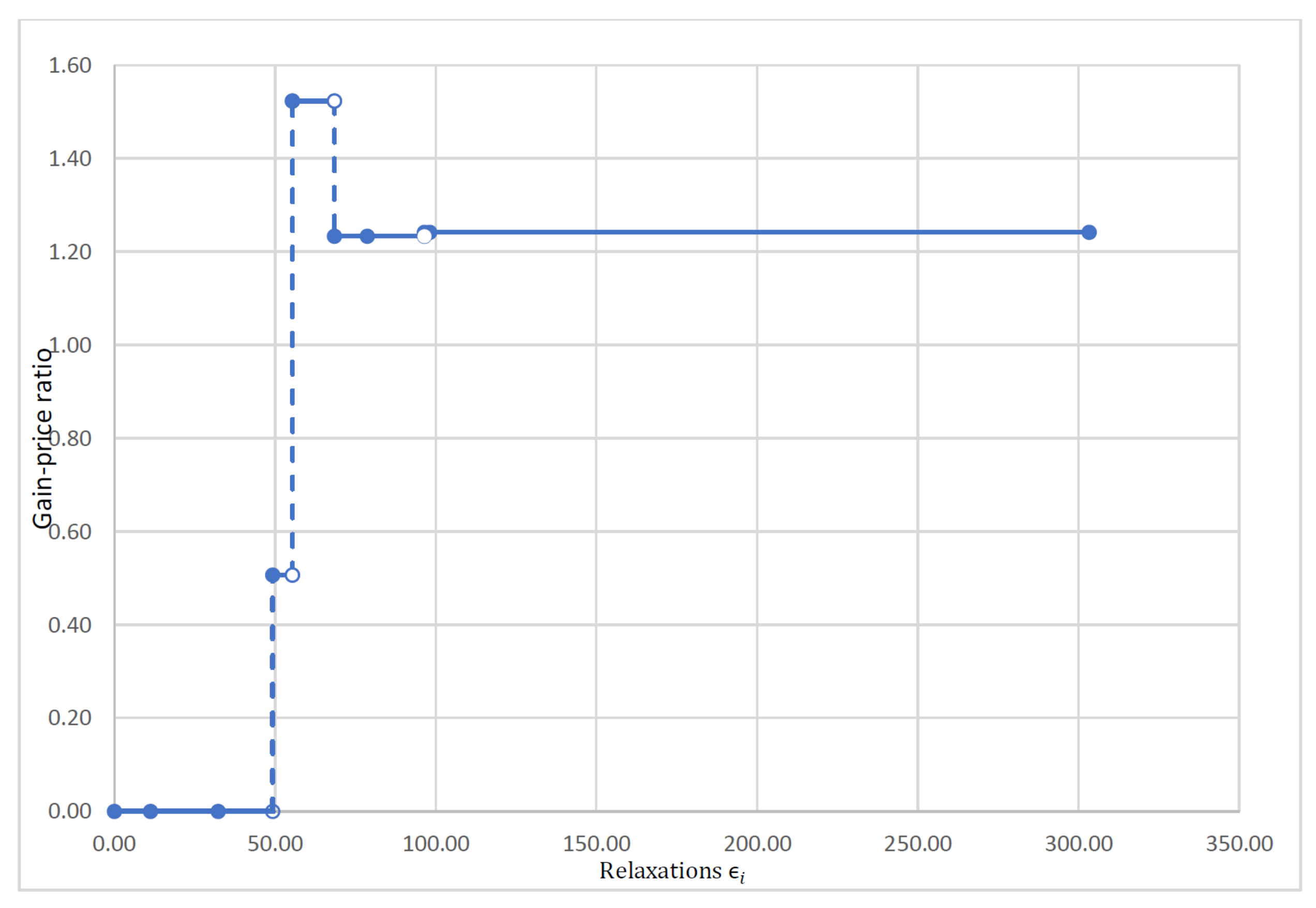
4.3. Trade-Off between the Gain of Robustness and the Price to Be Paid for Robustness

The following table shows a portion of a trade-off between the gain of robustness and the price to be paid for robustness for each solution set.
Remark 6.
(i)
As indicated in Table 3, the gain in robustness and the price to be paid for robustness of two solution sets X LRMOP ( s ^ , ε 1 ) * and X LRMOP ( s ^ , ε 2 ) * are 0. This is because of all solutions in these two sets being identical to the solution set X LRMOP ( s ^ , ε 0 ) * (see Appendix A for the explicit solutions information).
(ii)
For the three relaxations ε 4 , ε 5 , and ε 6 , the associated gain in robustness values is the same number, which is 84.42 . However, it was asserted that the price to be paid for robustness of these three solution sets are different. For the first set X LRMOP ( s ^ , ε 4 ) * , the value of the price to be paid for robustness is 55.43 , while the remaining two sets, X LRMOP ( s ^ , ε 5 ) * and X LRMOP ( s ^ , ε 6 ) * , are 68.44 . This is due to the fact that the new members in the sets X LRMOP ( s ^ , ε 5 ) * and X LRMOP ( s ^ , ε 6 ) * provided the value of the corresponding longest distance in the nominal problem more than the existing elements in the set X LRMOP ( s ^ , ε 4 ) * .
Based on the above discussion and information in Table 3, the question that could be raised to decision makers is which relaxation should be chosen. A direction that can be used for obtaining the answer is considering the trade-off between the gain in robustness and the price to be paid for robustness. Figure 2 shows the visualization of a trade-off in each level of robustness of the solution set.
Rationally speaking, the ratio of the gain in robustness and the price to be paid for the robustness means the benefits in robustness of solutions which we obtain and the nominal quality of the solutions we lose.
From Figure 2, we see that the highest ratio value of trade-off is 1.52 , which is obtained from solutions in the fifth level of robustness of the solution set X LRMOP ( s { 0 } , ε 4 ) * , where ε 4 = 55.43 . This means that the solution set of the fifth level of robustness can be considered the most desirable solution compared with another level of robustness set.
Remark 7.
(i)
An important point to note is that if we choose the optimal location pattern relying on just data on the nominal problem MP ( s { 0 } ) and ignore the uncertainty of unavailable ambulances, it is possible that the network components of the location pattern could lose functions when a disaster or crisis occurs in practice. In fact, for example, by choice of location pattern { A 2 , A 3 , A 8 , A 9 , A 12 } , which is an optimal solution in the nominal problem (there is neither disaster nor crisis), the longest distance covering all demand sites with respect to this location pattern is 193.24 units. However, if there is an unavailability of ambulances once a vehicle is dispatched to a call, then the longest distance covering all demand sites with respect to this location pattern { A 2 , A 3 , A 8 , A 9 , A 12 } in the worst-case scenario become 644.92 units. Note that the number of the longest distance covering all demand sites by the location pattern { A 2 , A 3 , A 8 , A 9 , A 12 } is worse than all optimal location patterns, which are computed by the concept of lightly robust max-ordering solution in the worst-case scenario (for more information see Table 2). This means that the benefits of a solution obtained by our proposed solution concept ensure a high performance in serving the longest distance covering all demand sites in uncertain environments.
(ii)
In the general setting on n candidate locations to locate r ambulances, we can calculate all possible scenarios of simultaneously unavailable ambulances by the formula:
1 + n r i = 1 r 1 r i

5. Conclusions

This research extended the concept of light robustness proposed by Fischetti and Monaci [19] from its original use in uncertain single-objective optimization problems to new use in uncertain multiobjective optimization problems. The new concept of the robust solution and a method of the solution’s computing were proposed in Section 2. This new solution concept is appropriate to a type of problem that required a solution which works well for solving issues that concern the maximum cost in the worst-case scenario with primary respect to the normal situation. We also analyzed the trade-off between nominal quality and robustness by proposing a measure for the price of robustness based on a lightly robust max-ordering solution concept in Section 3. This measurement can help a decision-maker to consider how much a nominal quality should be sacrificed in order to achieve a more desirable strength in a solution. So, it is appropriate for decision makers who are interested in a compromise between the robustness of solutions and the quality of solutions in a nominal scenario.
A numerical example was implemented in an ambulance location problem in Section 4. In the worst-case scenario, it showed that the set of solutions which are computed by using the lightly robust max-ordering solution always provided a better performance than the set of solutions that are obtained regardless of uncertainty. This argues that the proposed solution concept is a good direction when dealing with this kind of problem. It can be seen that the presented experimental and methodical details are provided so that the results can be reproduced for other interesting appropriate problems. It is worth noticing that the aim of the LRMOP ( s ^ , ε ) model (5) is exactly to pay attention to the nominal scenario and the worst-case scenario. Therefore, carefully gathering the information required for judging which scenarios to play in these two roles is very important because this can affect the final suggested solution. Furthermore (see Remark 7 (ii) for the discussion point), we see that the problem size for solving uncertain multiobjective optimization problems with respect to LRMOP ( s ^ , ε ) model (5) solution concept needs expensive computation. In fact, it is an NP-complete problem (see [2] for more detail), and this can affect the limitations of the applicability of the presented solution concept (5). According to this note, one may see that the idea of using techniques to make grouping scenarios, such as the clustering technique with respect to some factors, can be one future research direction to avoid expensive computation. Finally, for ease of applications of the solution concept presented in this paper, estimating the numerical effort resulting from the implementation of the methodology described in popular programming environments deserves consideration.

Author Contributions

Conceptualization, P.B., T.P. and N.P.; methodology, P.B., T.P. and N.P.; software, T.P.; validation, P.B., T.P. and N.P.; formal analysis, P.B., T.P. and N.P.; investigation, P.B., T.P. and N.P.; writing—original draft preparation, P.B.; writing—review and editing, P.B., T.P. and N.P.; supervision, N.P. All authors have read and agreed to the published version of the manuscript.

Funding

P.B. is supported by by the Thailand Research Fund through the Royal Golden Jubilee Ph.D. Program (Grant No. PHD/0046/2559) and N.P. is supported by the National Research Council of Thailand (Grant No. R2565B074).

Institutional Review Board Statement

Not applicable.

Informed Consent Statement

Not applicable.

Conflicts of Interest

The authors declare no conflict of interest.

Abbreviations

I p The index set { 1 , 2 , , p } , for each p N
R p The vector space with p dimension
R Set of real numbers
N Set of natural numbers
XSet of decision space
U Set of uncertainty
fObjective function
x R p A vector x with p coordinates, that is x = ( x 1 , x 1 , , x p )
A R p A subset A of vector space R p
I 10 
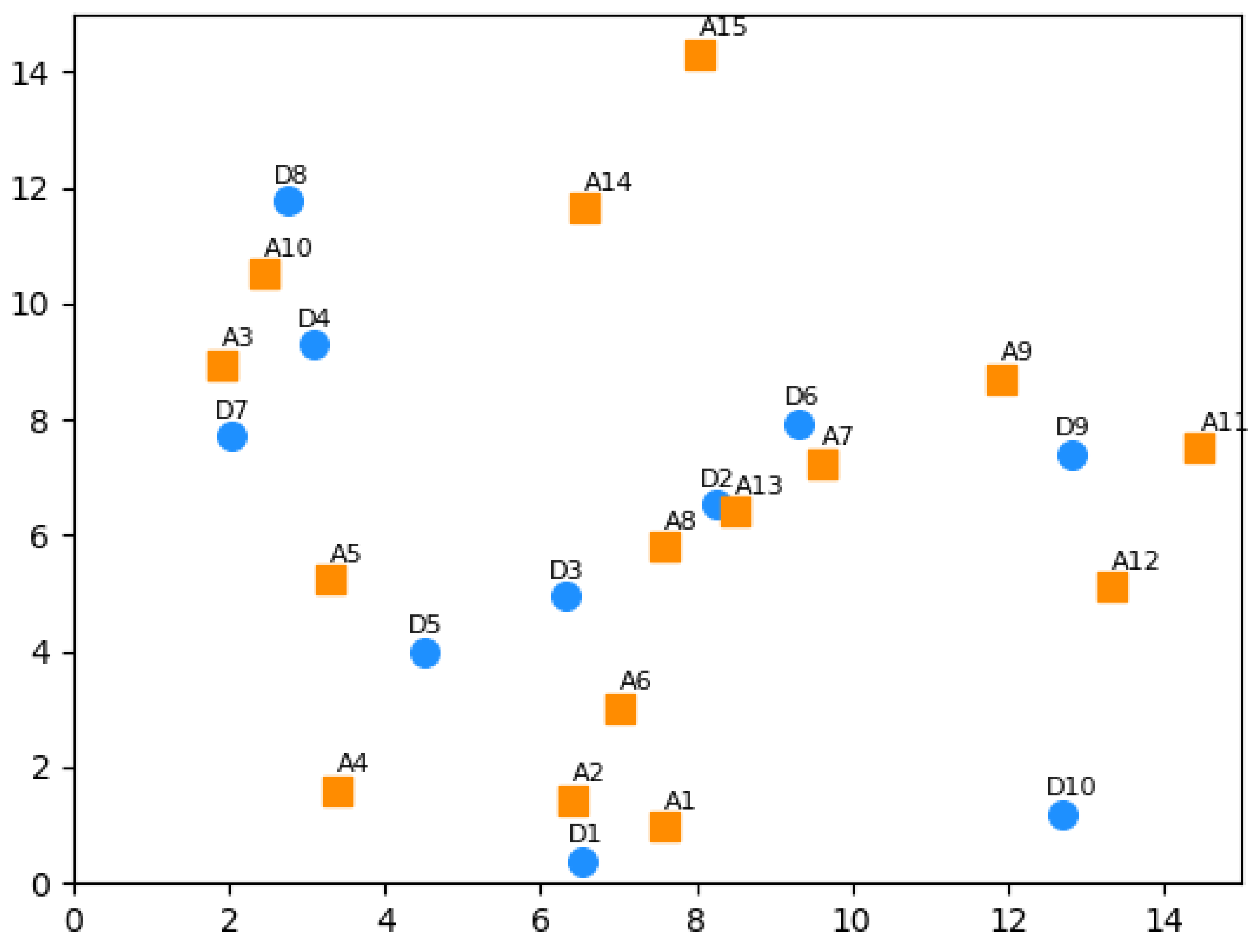
The index set of emergency demand sites
J 15 The index set of ambulance candidate locations
H 5 The index set of the considered ambulances
D i The emergency demand site i, where i I 10 (the blue squares)
d i The weight of emergency demand site D i , where i I 10 (the details on
each simulated data of d i can be found in Table 1)
A j The ambulance candidate location j, where j I 15 (the blue squares)
a k : = { a k 1 , a k 2 , a k 3 , a k 4 , a k 5 } the kth location pattern for the considered 5 ambulances.

Appendix A

Table A1. The optimal location patterns with different relaxations for the ambulance location problem.
Thresholds X LRMOP ( s { 0 } , ε m ) *
ε 0 , ε 1 , ε 2 [ 00.00 , 32.30 ] { A 1 , A 2 , A 5 , A 6 , A 12 }
{ A 1 , A 2 , A 5 , A 7 , A 12 }
{ A 1 , A 2 , A 5 , A 8 , A 12 }
{ A 1 , A 2 , A 5 , A 9 , A 12 }
{ A 1 , A 2 , A 5 , A 11 , A 12 }
{ A 1 , A 2 , A 5 , A 12 , A 13 }
{ A 1 , A 5 , A 6 , A 7 , A 12 }
{ A 1 , A 5 , A 6 , A 8 , A 12 }
{ A 1 , A 5 , A 6 , A 9 , A 12 }
{ A 1 , A 5 , A 6 , A 11 , A 12 }
{ A 1 , A 5 , A 6 , A 12 , A 13 }
{ A 1 , A 5 , A 7 , A 8 , A 12 }
{ A 1 , A 5 , A 7 , A 9 , A 12 }
{ A 1 , A 5 , A 7 , A 11 , A 12 }
{ A 1 , A 5 , A 7 , A 12 , A 13 }
{ A 1 , A 5 , A 8 , A 9 , A 12 }
{ A 1 , A 5 , A 8 , A 11 , A 12 }
{ A 1 , A 5 , A 8 , A 12 , A 13 }
{ A 1 , A 5 , A 9 , A 11 , A 12 }
{ A 1 , A 5 , A 9 , A 12 , A 13 }
{ A 1 , A 5 , A 11 , A 12 , A 13 }
{ A 2 , A 5 , A 6 , A 7 , A 12 }
{ A 2 , A 5 , A 6 , A 8 , A 12 }
{ A 2 , A 5 , A 6 , A 9 , A 12 }
{ A 2 , A 5 , A 6 , A 11 , A 12 }
{ A 2 , A 5 , A 6 , A 12 , A 13 }
{ A 2 , A 5 , A 7 , A 8 , A 12 }
{ A 2 , A 5 , A 7 , A 9 , A 12 }
{ A 2 , A 5 , A 7 , A 11 , A 12 }
{ A 2 , A 5 , A 7 , A 12 , A 13 }
{ A 2 , A 5 , A 8 , A 9 , A 12 }
{ A 2 , A 5 , A 8 , A 11 , A 12 }
{ A 2 , A 5 , A 8 , A 12 , A 13 }
{ A 2 , A 5 , A 9 , A 11 , A 12 }
{ A 2 , A 5 , A 9 , A 12 , A 13 }
{ A 2 , A 5 , A 11 , A 12 , A 13 }
{ A 5 , A 6 , A 7 , A 8 , A 12 }
{ A 5 , A 6 , A 7 , A 9 , A 12 }
{ A 5 , A 6 , A 7 , A 11 , A 12 }
{ A 5 , A 6 , A 7 , A 12 , A 13 }
{ A 5 , A 6 , A 8 , A 9 , A 12 }
{ A 5 , A 6 , A 8 , A 11 , A 12 }
{ A 5 , A 6 , A 8 , A 12 , A 13 }
{ A 5 , A 6 , A 9 , A 11 , A 12 }
{ A 5 , A 6 , A 9 , A 12 , A 13 }
{ A 5 , A 6 , A 11 , A 12 , A 13 }
{ A 5 , A 7 , A 8 , A 9 , A 12 }
{ A 5 , A 7 , A 8 , A 11 , A 12 }
{ A 5 , A 7 , A 8 , A 12 , A 13 }
{ A 5 , A 7 , A 9 , A 11 , A 12 }
{ A 5 , A 7 , A 9 , A 12 , A 13 }
{ A 5 , A 7 , A 11 , A 12 , A 13 }
{ A 5 , A 8 , A 9 , A 11 , A 12 }
{ A 5 , A 8 , A 9 , A 12 , A 13 }
{ A 5 , A 8 , A 11 , A 12 , A 13 }
{ A 5 , A 9 , A 11 , A 12 , A 13 }
ε 3 = 49.21 { A 1 , A 2 , A 6 , A 8 , A 12 }
{ A 1 , A 2 , A 7 , A 8 , A 12 }
{ A 1 , A 2 , A 8 , A 9 , A 12 }
{ A 1 , A 2 , A 8 , A 12 , A 13 }
{ A 1 , A 6 , A 7 , A 8 , A 12 }
{ A 1 , A 6 , A 8 , A 9 , A 12 }
{ A 1 , A 6 , A 8 , A 12 , A 13 }
{ A 1 , A 7 , A 8 , A 9 , A 12 }
{ A 1 , A 7 , A 8 , A 12 , A 13 }
{ A 1 , A 8 , A 9 , A 12 , A 13 }
{ A 2 , A 6 , A 7 , A 8 , A 12 }
{ A 2 , A 6 , A 8 , A 9 , A 12 }
{ A 2 , A 6 , A 8 , A 12 , A 13 }
{ A 2 , A 7 , A 8 , A 9 , A 12 }
{ A 2 , A 7 , A 8 , A 12 , A 13 }
{ A 2 , A 8 , A 9 , A 12 , A 13 }
{ A 6 , A 7 , A 8 , A 9 , A 12 }
{ A 6 , A 7 , A 8 , A 12 , A 13 }
{ A 6 , A 8 , A 9 , A 12 , A 13 }
{ A 7 , A 8 , A 9 , A 12 , A 13 }
ε 4 = 55.43 { A 1 , A 6 , A 7 , A 8 , A 9 }
{ A 1 , A 6 , A 7 , A 8 , A 13 }
{ A 1 , A 6 , A 8 , A 9 , A 13 }
{ A 1 , A 7 , A 8 , A 9 , A 13 }
ε 5 = 68.44 { A 1 , A 6 , A 7 , A 8 , A 9 }
{ A 1 , A 6 , A 7 , A 8 , A 13 }
{ A 1 , A 6 , A 7 , A 9 , A 13 }
{ A 1 , A 6 , A 8 , A 9 , A 13 }
{ A 1 , A 7 , A 8 , A 9 , A 13 }
ε 6 = 78.74 { A 1 , A 6 , A 7 , A 8 , A 9 }
{ A 1 , A 6 , A 7 , A 8 , A 13 }
{ A 1 , A 6 , A 7 , A 9 , A 13 }
{ A 1 , A 6 , A 8 , A 9 , A 13 }
{ A 1 , A 7 , A 8 , A 9 , A 13 }
ε 7 = 96.45 { A 6 , A 7 , A 8 , A 9 , A 13 }
ε 8 = 98.10 { A 6 , A 7 , A 8 , A 9 , A 13 }
ε 9 = 303.25 { A 6 , A 7 , A 8 , A 9 , A 13 }

References

  1. Schmidt, M.; Schöbel, A.; Thom, L. Min-ordering and max-ordering scalarization methods for multiobjective robust optimization. Eur. J. Oper. Res. 2019, 275, 446–459. [Google Scholar] [CrossRef]
  2. Ehrgott, M. Location of Rescue Helicopters in South Tyrol. Int. J. Ind. Eng. 2001, 9, 16–22. [Google Scholar]
  3. Toregas, C.; Swain, R.; ReVelle, C.; Bergman, L. The location of emergency service facilities. Oper. Res. 1971, 19, 1363–1373. [Google Scholar] [CrossRef]
  4. Church, R.; ReVelle, C. The maximal covering location problem Papers in Regional Science. Pap. Reg. Sci. Assoc. 1974, 32, 101–118. [Google Scholar] [CrossRef]
  5. Schmid, V.; Doerner, K.F. Ambulance location and relocation problems with time- dependent travel times. Eur. J. Oper. Res. 2010, 207, 1293–1303. [Google Scholar] [CrossRef] [Green Version]
  6. Li, X.; Zhao, Z.; Zhu, X.; Wyatt, T. Covering Models and Optimization Techniques for Emergency Response Facility Location and Planning: A Review. Math. Methods Oper. Res. 2011, 74, 281–310. [Google Scholar] [CrossRef]
  7. Lee, G.; Murray, A.T. Maximal Covering with Network Survivability Requirements in Wireless Mesh Networks. Comput. Environ. Urban Syst. 2010, 34, 49–57. [Google Scholar] [CrossRef]
  8. Snyder, S.; Haight, R.G. Application of the maximal covering location problem to habitat reserve site selection: A review. Int. Reg. Sci. Rev. 2016, 39, 28–47. [Google Scholar] [CrossRef] [Green Version]
  9. Li, M.; Xie, C.; Li, X.; Karoonsoontawong, A.; Ge, Y.E. Robust liner ship routing and scheduling schemes under uncertain weather and ocean conditions. Transp. Res. Part C Emerg. Technol. 2022, 137, 103593. [Google Scholar] [CrossRef]
  10. Gao, H.; Xin, X.; Li, C.; Liu, Y.; Chen, K. Container ocean shipping network design considering carbon tax and choice inertia of cargo owners. Ocean Coast. Manag. 2022, 216, 105986. [Google Scholar] [CrossRef]
  11. Ben-tal, A.; Nemirovski, A.T. Robust convex optimization. Math. Oper. Res. 1998, 23, 769–805. [Google Scholar] [CrossRef] [Green Version]
  12. Ben-Tal, A.; Ghaoui, L.E.; Nemirovski, A. Robust Optimization; Princeton University Press: Princeton, NJ, USA, 2009. [Google Scholar]
  13. Kuroiwa, D.; Lee, G.M. On robust multiobjective optimization. Vietnam J. Math. 2012, 40, 305–317. [Google Scholar]
  14. Ehrgott, M.; Ide, J.; Schöbel, A. Minmax robustness for multiobjective optimization problems. Eur. J. Oper. Res. 2014, 239, 13–17. [Google Scholar] [CrossRef]
  15. Fliege, J.; Werner, R. Robust Multiobjective Optimization and Applications in Portfolio Optimization. Eur. J. Oper. Res. 2014, 234, 422–433. [Google Scholar] [CrossRef]
  16. Wei, H.-Z.; Chen, C.-R.; Li, S.-J. Characterizations of multiobjective robustness on vectorization counterparts. Optimization 2020, 182, 466–493. [Google Scholar] [CrossRef]
  17. Boriwan, P.; Ehrgott, M.; Kuroiwa, D.; Petrot, N. The lexicographic tolerable robustness concept for uncertain multiobjective optimization problems: A study on water resources management. Sustainability 2020, 12, 7582. [Google Scholar] [CrossRef]
  18. Boriwan, P.; Kuroiwa, D.; Petrot, N. On the properties of lexicographic tolerable robust solution sets for uncertain multiobjective optimization problems. Carpathian J. Math. 2021, 12, 25–34. [Google Scholar]
  19. Fischetti, M.; Monaci, M. Light robustness. In Robust and Online Large-Scale Optimization; Springer: Berlin/Heidelberg, Germany, 2009; pp. 61–84. [Google Scholar]
  20. Kuhn, K.; Raith, A.; Schmidt, M.; Schöbel, A. Bi-objective robust optimisation. Eur. J. Oper. Res. 2016, 252, 418–431. [Google Scholar] [CrossRef]
  21. Ide, J.; Schöbel, A. Robustness for uncertain multiobjective optimization: A survey and analysis of different concepts. OR Spectr. 2016, 38, 235–271. [Google Scholar] [CrossRef]
  22. Schöbel, A.; Zhou-Kanges, Y. The price of multiobjective robustness: Analyzing solution sets to uncertain multiobjective problems. Eur. J. Oper. Res. 2021, 291, 782–793. [Google Scholar] [CrossRef]
  23. Ehrgott, M. Multiobjective Optimization; Springer: Berlin/Heidelberg, Germany, 2005. [Google Scholar]
  24. Fiacco, A.V.; McCormick, G.P. Nonlinear Programming: Sequential Unconstrained Minimization Techniques; John Wiley Sons: New York, NY, USA, 1968. [Google Scholar]
  25. Horst, R.; Tuy, H. Global Optimization: Deterministic Approaches, 3rd ed.; Springer: Berlin/Heidelberg, Germany, 1995. [Google Scholar]
  26. Nimana, N.; Petrot, N. Splitting proximal with penalization schemes for additive convex hierarchical minimization problems. Optim. Methods Softw. 2020, 35, 1098–1118. [Google Scholar] [CrossRef]
  27. Nimana, N.; Petrot, N. Generalized forward-backward splitting with penalization for monotone inclusion problems. J. Glob. Optim. 2019, 73, 825–847. [Google Scholar] [CrossRef] [Green Version]
  28. Petrot, N.; Nimana, N. Incremental proximal gradient scheme with penalization for constrained composite convex optimization problems. Optimization 2021, 70, 1307–1336. [Google Scholar] [CrossRef]
Figure 1. Ambulance locations and potential demand sites.
Sustainability 14 07511 g001
Figure 2. The ratios G P of the gain in robustness and the price to be paid for robustness corresponding to different relaxations ε m [ 00.00 , + ) .
Sustainability 14 07511 g002
Table 1. Weight of demand site D i for i I 10 of the ambulance location problem.
Demand SitesWeight d i of Demand Site D i
D 1 27.21040801
D 2 4.10474611
D 3 18.31712008
D 4 42.5425252
D 5 20.31375215
D 6 1.36011829
D 7 12.35886195
D 8 3.35721854
D 9 49.69260057
D 10 48.52901567
Table 2. Computational experiments of the problem LRMOP ( s { 0 } , ε m ) where ε m are computed as in Theorem 1.
RelaxationOptimal Values
ε 0 = 00.00 496.49
ε 1 = 11.15 496.49
ε 2 = 32.30 496.49
ε 3 = 49.21 471.60
ε 4 = 55.43 412.07
ε 5 = 68.44 412.07
ε 6 = 78.74 412.07
ε 7 = 96.45 376.69
ε 8 = 98.10 376.69
ε 9 = 303.25 376.69
Table 3. The gain of robustness and the price to be paid for robustness with respect to each ε m [ 0.00 , + ) .
RelaxationTrade-Off
GainPriceRatio
( G ) ( P ) G P
ε 0 = 00.00 000
ε 1 = 11.15 000
ε 2 = 32.30 000
ε 3 = 49.21 24.9049.210.5
ε 4 = 55.43 84.4255.431.52
ε 5 = 68.44 84.4268.441.23
ε 6 = 78.74 84.4268.441.23
ε 7 = 96.45 119.8096.451.24
ε 8 = 98.10 119.8096.451.24
ε 9 = 303.25 119.8096.451.24
Publisher’s Note: MDPI stays neutral with regard to jurisdictional claims in published maps and institutional affiliations.

