Article

Spatial–Temporal Variations of Water Ecosystem Services Value and Its Influencing Factors: A Case in Typical Regions of the Central Loess Plateau

State Key Laboratory of Eco-Hydraulics in Northwest Arid Region, Xi’an University of Technology, Xi’an 710048, China
*
Author to whom correspondence should be addressed.
Sustainability 2022, 14(12), 7169; https://doi.org/10.3390/su14127169
Submission received: 9 May 2022 / Revised: 5 June 2022 / Accepted: 9 June 2022 / Published: 11 June 2022
(This article belongs to the Topic Water Management in the Era of Climatic Change)

Abstract

:
Water resources provide indispensable ecosystem services, which are related to human well-being and sustainable social development. Accurately measuring the water ecosystem services value (WESV), and then grasping its changing characteristics, is particularly important for solving water problems. In this study, the typical area of the central Loess Plateau location is taken as the research area. Based on remote sensing images and statistical data, the direct market method combined with the equivalent factor method was used to calculate the WESV including groundwater and surface water, which is of greatest originality. The temporal and spatial variation characteristics in 2010, 2015 and 2020 were analyzed. Then, four WESV driving factors including per capita GDP, population density, proportion of water areas, and water consumption were selected, and the geographically weighted regression (GWR) model was used to analyze the spatial distribution pattern and temporal variation of WESV’s response to the influencing factors. The results showed that WESV experienced a process of first decreasing and then increasing, which was mainly caused by Yulin. For the composition of WESV, the proportion of provisioning services value has increased, which caused the proportion of regulating services value to decrease. The correlations between four factors and WESV were different. The distribution pattern of the influences was spatially heterogeneous, which showed regular variations over time. These results indicate the necessity of WESV’s independent research and provide a realistic basis for ecological compensation in the Yellow River Basin.

1. Introduction

Ecosystems provide basic and necessary services for human survival and social functioning, namely ecosystem services (ESs). ESs are the continuous provision of ecosystem goods and services by ecosystems and their ecological processes [1]. However, factors such as population growth, industrialization and urbanization have led to a rapid increase in the demand for ESs, and ecosystems are facing unprecedented pressure [2]. A comprehensive and reasonable quantitative assessment of ecosystem services value (ESV) is necessary to alleviate the contradiction between supply and demand of ESs, manage effectively and formulate relevant policies. Water resources are an essential part of ecosystems. Whereas, due to the existence of water pollution, waste of water resources and climate change, the water ecosystem is facing greater pressure than other types of ecosystems. Therefore, it is crucial to study the water ecosystem services value (WESV) and the various factors that affect WESV.
Monetization of ecosystem service value is the most recognized and practical form of ESV, and the calculation methods can be divided into two categories. One is to adopt the relevant methods of traditional ecological economics or environmental economics. Most of these methods obtain the output of physical quantity based on statistical data or ecological model, and then they calculate the value of ecosystem services by combining the market value method, willingness survey method (CV) and revealed preference method. This kind of method has high requirements on data, parameters, model accuracy and method applicability, etc. Specific to the value of water resources ecosystem services, this kind of method is suitable for calculating the value of water resources with commodity attributes. The other is the equivalence factor method, which constructs the economic value equivalent per unit area of different ecosystems based on the division of ecosystem service functions and quantifies ESV in combination with the distribution of ecosystems. Compared with traditional methods, the equivalence factor method requires relatively fewer data, and the evaluation of ESVs is more comprehensive. Costanza et al. divided the global ESs into 17 species and calculated that the ESV of 16 biomes in the world was US$33 trillion per year [
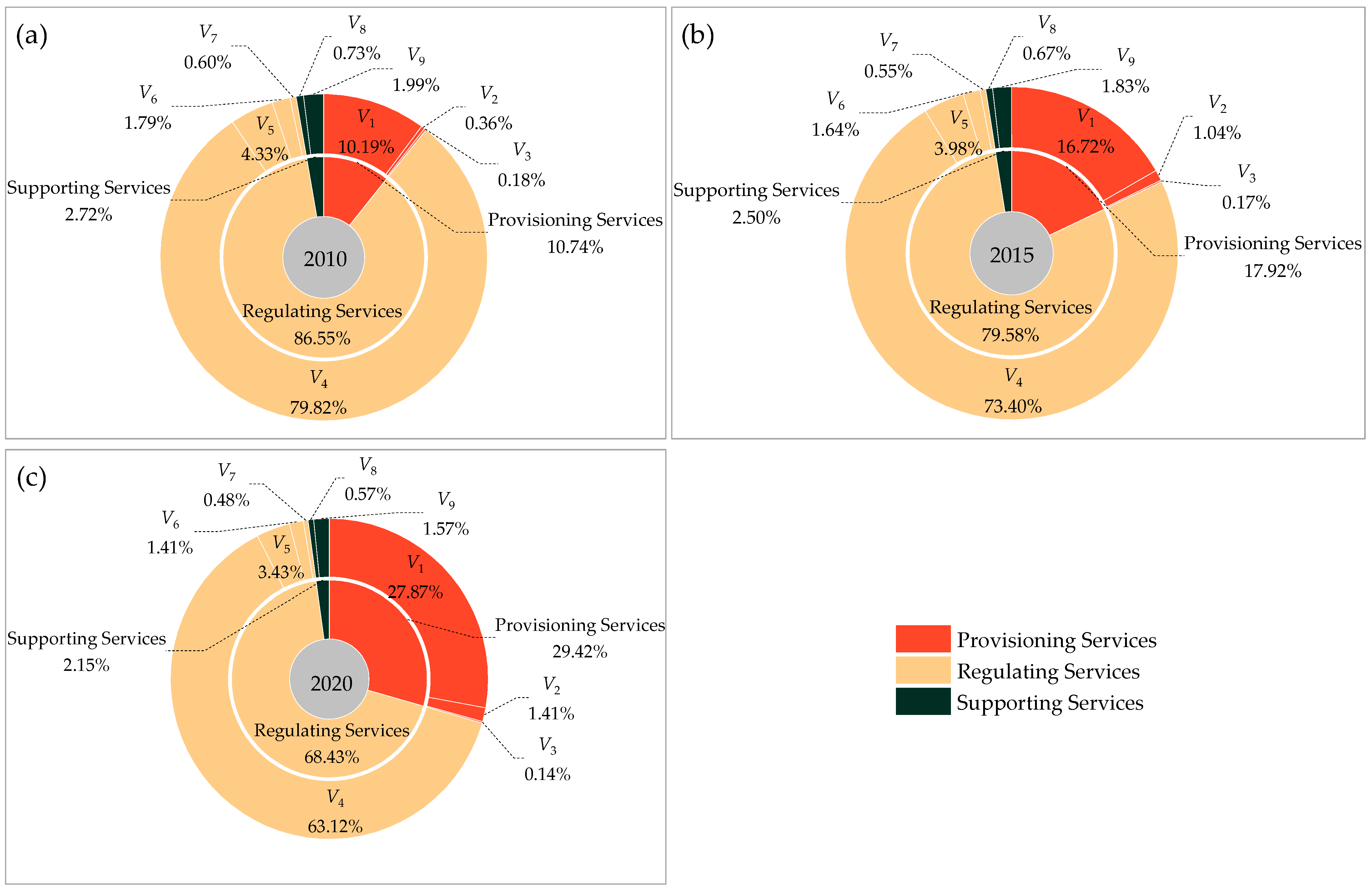
3], and rivers or lakes were one of the 16 biomes. Meanwhile, another contribution of this study is to provide the equivalent table of services value per unit area of 17 ecosystems in each biome at the global scale, which provides a reference for future research. In 2003, the Millennium Ecosystem Assessment (MA) conducted by the United Nations classified global ESs into four primary categories, namely Provisioning Services, Regulating Services, Supporting Services, and Cultural Services [4]. At the regional scale, Xie et al. improved Costanza’s research and obtained the equivalent factor of ecosystem service value suitable for China. Then, the ESV can be calculated combined with the area of each ecosystem. This study was accepted by a large number of Chinese scholars [5,6]. Whether it is a global scale or a regional scale, in the study of using the equivalent factor method to evaluate ecosystems, most of the rivers/lakes or waters are divided into one type of ecosystem for discussion. However, this method does not clarify the service value of groundwater, which is an important component of water resources. The most direct service value of groundwater is that it provides a part of water for production and domestic use, accounting for only 70% of the total global water use for agriculture, and 40% of agricultural water comes from groundwater [7]. Therefore, it is more comprehensive and accurate to combine the two methods to assess the WESV including surface water and groundwater.
It is not the ultimate goal of scholars to study the value of WESV; the more important goal is to study the relationship between WESV and the interaction of various factors. In order to deal with more severe water and environmental problems, exploring the influence of various factors on WESV has gradually become one of the research hotspots. Due to the social nature of water resources, social and economic factors have become one of the components that affect WESV. The characteristics of cities, populations, communities, and cultures [8] all have an impact on water resources and water ecology [9,10]. The urbanization level is a concentrated expression of the social and economic development degree, which profoundly affects the spatial distribution and potential functions of ecosystem services [11]. Many researchers have conducted related research in North China [12,13], Yangtze River Delta [14], Pearl River Delta [15], Southwest Mountainous [16,17] and Northwest arid regions of China [18,19]. WESV also has a significant response to changes in natural factors. Climate conditions [20,21,22], ecosystem types [23], and environmental quality [24] are the main influencing factors. Meanwhile, the coupling of many factors, such as nature, social economy and human activities, has a more realistic impact on WESV [25,26]. Many of the above studies have fully considered various factors and provided important references for explaining the changes caused by EVS or WESV. Unfortunately, the collinearity among some influencing factors and the nonstationarity in space have not attracted enough attention.
However, EVS exhibit spatial heterogeneity and spatial dependence with changes in geographic space due to differences in the socioeconomic development degree, natural resources, and geographic environment. Thus, incorporating geospatial aspects into the research scope is the key to addressing spatial heterogeneity. Geographically Weighted Regression (GWR) model is an effective tool for dealing with spatial heterogeneity, which is improved on the basis of ordinary least square [27]. The model incorporates the spatial location information as a coefficient into the regression equation and explores to eliminate the nonstationarity caused by spatial changes based on the fitted values of geographic element parameters [28]. The GWR model has been widely used in the fields of natural resources and ecological environment [29]. The water footprint has been extensively researched, including concepts, methods and applications, for better management of water resources and water ecology [30,31]. With the deterioration of ecological environment problems, it is necessary to analyze the evolution of ecological footprint and the spatial differences of influencing factors from the perspective of spatial heterogeneity [29]. In the related research on land use variation and ESV, the GWR model is used to solve the problem of spatial heterogeneity and compare with the OLS model [32]. In coastal counties of Mississippi and Alabama (U.S.), GWR was used in the estimation of the monetary value of distance to different waterfront types, in the extension to a traditional hedonic pricing method, and in analyzing the value of ecosystem services associated with waterfronts differed geospatially [33]. However, few researches utilize the GWR model to study WESV, which becomes the main content of this study.
In arid and semi-arid regions, water resources are very precious, which means that the ecological services provided by water resources play a vital role. Therefore, on the basis of accurately measuring the value of water resources ecosystem services, analyzing the impact of various factors on WESV is of great significance to effectively manage water resources and alleviate the contradiction between supply and demand of water resources ecosystem services.
Many studies have been conducted on the value of ecological services and their influencing factors. However, this study is more relevant. Specifically, the ecological service value of water resources is the object of this study. In addition, the scope of water resources is broader to include groundwater and surface water. This study serves the ecological compensation policy in China.
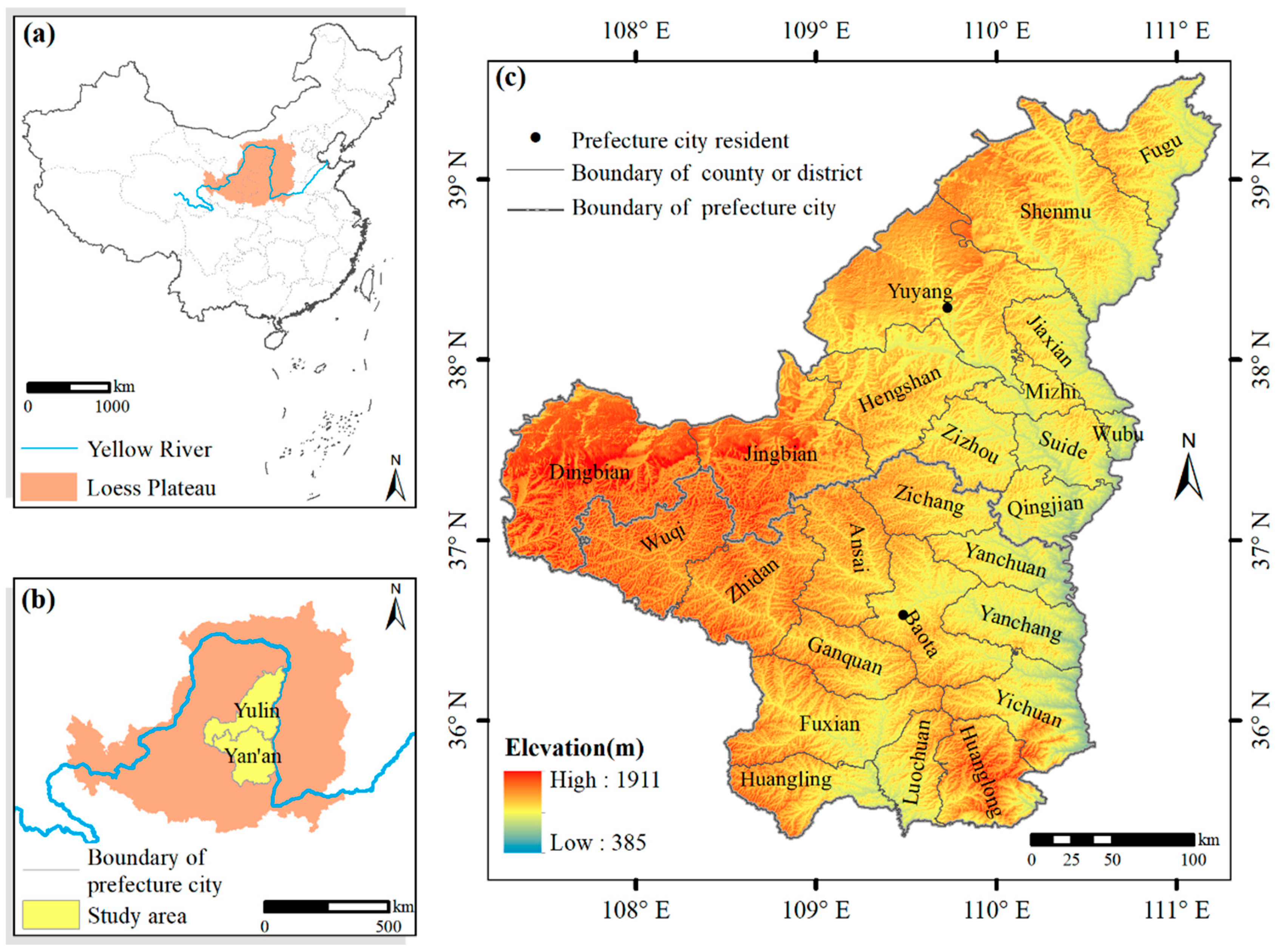
In this study, the typical area in the central Loess Plateau of China was taken as the research object, and the evaluation of water resources ecosystem service value and the analysis of the temporal and spatial changes of the influencing factors were carried out. The main works are as follows:
(1)
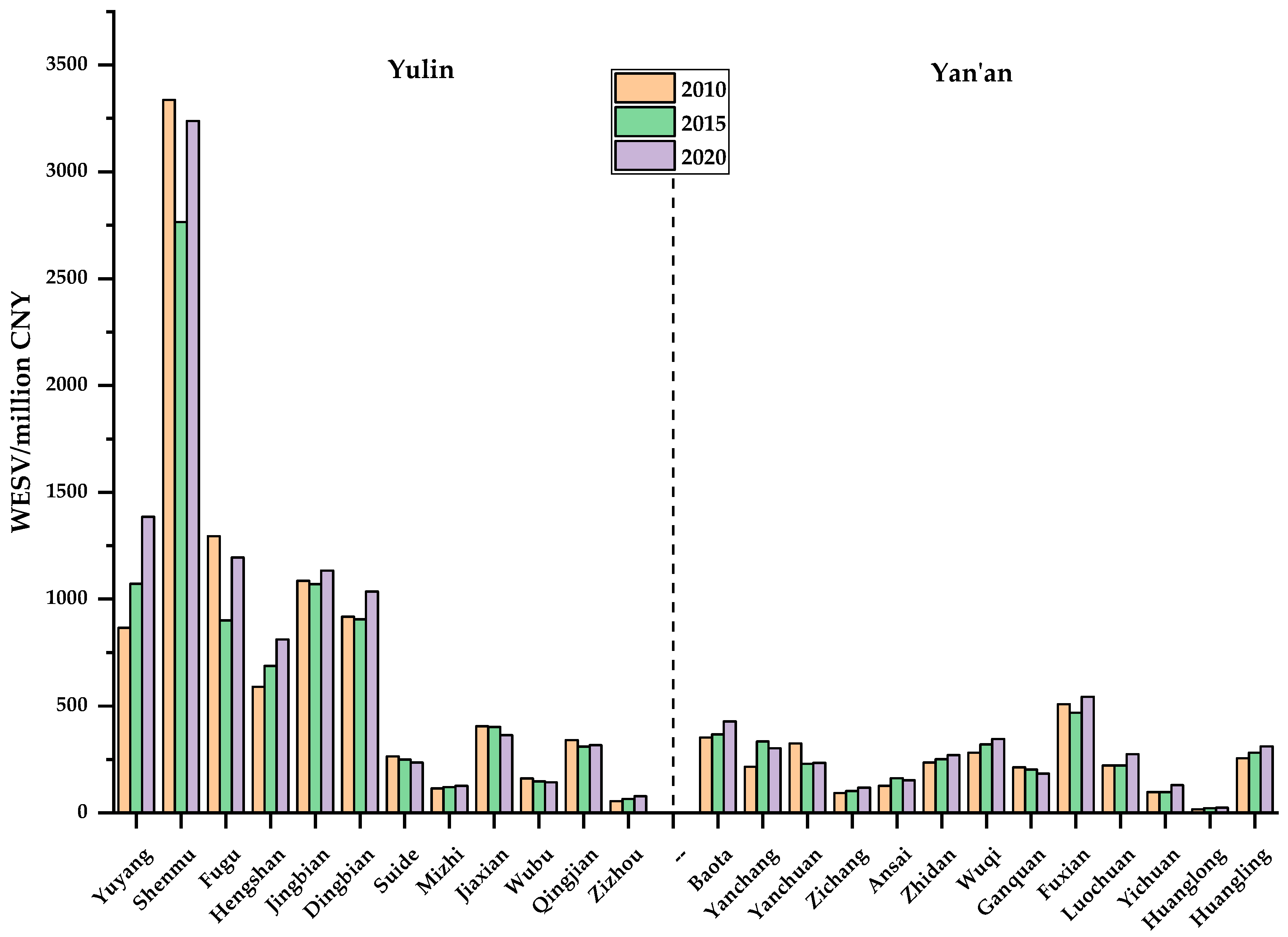
Combining the environmental economics method and the equivalent factor method, the WESVs of 25 counties (districts) in the study area including groundwater and surface water in 2010, 2015 and 2020 were calculated, and the distribution characteristics were analyzed;
(2)
Selecting the representative factors of nature, economy and society, and the applicability of OLS model and GWR model in studying the impact of each indicator on WESV was analyzed;
(3)
Using the more applicable GWR model, the spatial heterogeneity and spatial and temporal distribution of the effects of various factors on WESV were shown.

2. Materials and Methods

2.1. Study Area

The Loess Plateau (33°43′–41°160′ N, 100°54′–114°33′ E) covers an area of 640,000 km2 in the upper and middle reaches of China’s Yellow River (Figure 1a) [34,35]. Most areas of the Loess Plateau belong to arid and semi-arid areas, with fragile environment, scarcity of water resources and serious soil erosion [36,37]. The study area of this paper is Yulin and Yan’an Cities (Figure 1b), with an area of about 79,957 km2, accounting for 12.49% of the area of the Loess Plateau. In terms of location, the study area is located in the middle of the Loess Plateau, which is a representative area in the middle of the Loess Plateau. From the perspective of administrative division, the study area belongs to the north of Shaanxi Province. The study area includes 25 county-level administrative units (Figure 1c). The study area with large topographic relief and hilly gully, is the core area for controlling soil and water loss in the Yellow River Basin. The annual average temperature of Yulin City in the north of the study area is about 10.5 °C, and the average annual precipitation is about 400.00 mm. From north to south, the landform gradually transits from sandy land to gullies and hills [38,39]. It is an important energy and chemical base in China. Yan’an City in the south of the study area belongs to the hilly area of the Loess Plateau, which is high in the northwest and low in the southeast. The annual average temperature is about 7.70~10.60 °C, and the annual average precipitation is about 500.00 mm [40,41,42].

2.2. Data Sources

The data involved in this study include economic indicators, social indicators, and natural indicators of Yulin and Yan’an Cities in 2010, 2015 and 2020. It should be noted that due to the impact of COVID-19, some economic and social indicators in 2020 are replaced by data from 2019, including population, population density, urbanization rate, per capital GDP, and gross product of primary industry.
The water consumption comes from the water resources bulletin of Yulin and Yan’an Cities (2010, 2015 and 2020). Through reclassification, water consumption is divided into three categories: agricultural water consumption, residential water consumption and nonresidential water consumption. The price of water is obtained from the research of the water supply department.
GDP, GDP per capita, population, population density and urbanization rate are from the statistical yearbooks of Yulin and Yan’an (2010, 2015 and 2019).
The water area and the proportion of water area are calculated through the statistical calculation of the spatial distribution data of the national land use type remote sensing monitoring provided by the Resource and Environmental Science and Data Center, Chinese Academy of Sciences (http://www.resdc.cn/, accessed on 2 July 2018). The resolution of the data is 30 m × 30 m, which is generated by manual visual interpretation using the remote sensing images of Landsat TM of various phases of the US Landsat as the main data source.

2.3. Methods

2.3.1. Classification and Calculation Method of WESV

According to the classification of ESs by the Millennium Ecosystem Assessment (MA 2005) carried out by the United Nations [4], combined with the research practice in China [43] and the practicability of ecological compensation in the study area, this study divided WESV into three categories. The reason why the cultural services value was not considered is that at this stage, ecological compensation in China rarely involves such services value. Considering the ways of WES and the availability of data, the three categories were subdivided into 9 specific services (Table 1). The calculation method of WESV can be expressed formally as follows:
V w = n = 1 9 V n
where Vw is the value of WESV; Vn is the n-th sub-category of WESV; n = 1, 2, …, 9.

2.3.2. Market Value Method

Whether groundwater or surface water, the most direct and important service is water supply for living and production. The value of water services is reflected in the water price [44]. Therefore, this study adopts the market value method to calculate the water supply services value of water resources. According to the type of water price, water is divided into agricultural water, residential water and nonresidential water, among which nonresidential water mainly refers to industrial, business service water, administrative institution water, municipal water, etc. The formula for calculation is as follows:
V 1 = j = 1 3 Q j × P j ,
where V1 is the value of water supply services; Qj and Pj are the water consumption and water price of the j-th type of water; j = 1, 2, 3 represent agricultural water, residential water and nonresidential water, respectively.
The market value method is also used to calculate the indirect supply value of aquatic products provided by water resources. Due to the variety of aquatic products and the different prices, this study uses the fishery output value in the statistical yearbook [45,46,47,48] as the value V2 of aquatic product supply services, and the calculation method also adopts the market value method.

2.3.3. Equivalent Factor Method

Water resources are the most basic elements to maintain the normal operation of ecosystems and social systems, and most of its ecosystem services cannot be measured by market value. The ESV equivalent factor method is obtained from the study of Xie G. [5] by calculating the ecological service value per unit area of each ecosystem in China, which has been widely recognized and applied [49]. The equivalence factor is defined as a relative quantity, which represents a relative value of ecosystem services relative to the economic value of grain output in that year. In the case of the study area, due to the difference in planting structure, the economic value of grain output will change accordingly. The ecological service value of the study area can be calculated by the follows:
V p e r = 1 7 × Y 1 × P 1 + Y 2 × P 2 A 1 + A 2 ,
where Vper is the value of ESs per unit area; corn and potato are mainly planted in the study area, Y1 and Y2 are the yield of corn and potato, respectively, which comes from “Shaanxi Statistical Yearbook” [45,46,47,48]; P1 and P2 are the corresponding grain prices, which comes from “Compilation of National Agricultural Product Cost and Benefit Data” [50,51,52]; A1 and A2 are the planting area of corresponding grain; 1/7 is the ratio of the economic value provided by natural ecosystems without artificial inputs to the economic value provided by existing farmland. The calculated values of ESs per unit area in 2010, 2015 and 2020 were 1457.16 CNY/hm2, 1318.81 CNY/hm2 and 1199.63 CNY/hm2, respectively.
The equivalence factor adopts the corresponding part of the water ecosystem in the equivalence coefficient table of ecosystem service value per unit area calculated by Xie G. [43] (Table 2). At the same time, the value of WESV per unit area in 2010, 2015 and 2020 was calculated (Table 2).
Then, the value of services other than Water supply and Aquatic product could be calculated as follows:
V m = V p e r × A w × E m ,
where m = 3, 4, 5, …, 9; Vm is the value of other services besides Water supply and Aquatic product; Aw represents the watershed area for the study year; Em is the equivalent coefficient of different service in Table 2.

2.3.4. Geographically Weighted Regression

The first law of spatial geography shows that the correlation between ground objects gradually increases as the distance decreases [53,54]. Inevitably, spatial correlation and spatial heterogeneity coexist. GWR achieves better results when using local smoothing to deal with the problem of spatial heterogeneity [55,56]. GWR was based on kernel-weighted regression. Instead of estimating global values for regression parameters, GWR allows these parameters to be derived for each location separately [57]. The model can be expressed as
y i = β 0 μ i , ν i + k β k μ i , ν i x i , k + ε i ,
where yi is the explained variable; (μi, νi) are the coordinates of the target area i; β0 (μi, νi) is the intercept; xi,k is the value of the explanatory variable xk on the target area i; the value of the function βk (μi, νi) at geographic location i is βk (μi, νi); k is the number of explanatory variables; εi is the random disturbance term, i.e., the error. The coefficient of each sample point is a parameter estimate obtained by weighting the adjacent observations [58], and the expression is as follows:
β ^ ( u i ,   v i ) = ( X T W ( u i ,   v i ) X ) 1 X T W ( u i ,   v i ) Y ,
where β ^ ( u i ,   v i ) is the parameter estimate of the local coefficient of the i-th sample with coordinates (μi, νi); X and Y are the vectors of the explanatory and the dependent variables; W ( u i ,   v i ) is the weight matrix, which is usually calculated by the Gaussian function of the distance decay function (kernel function).
ArcGIS software has developed the related functions of OLS and GWR into convenient tools. Therefore, this study uses ArcGIS 10.4 to perform related calculations.

3. Results

3.1. WESVs and Characteristics in 2010–2020

3.1.1. Temporal and Spatial Variation Analysis of WESV

Taking the county-level administrative region as the minimum calculation unit, and adopting appropriate methods according to different service types, the WESVs of typical areas in the middle of the Loess Plateau in 2010, 2015 and 2020 were calculated (Table 3). The changes in counties among the three years have also been shown (Figure 2). Overall, the WESV in the study area showed a trend of first decreasing and then increasing. The WESV decreased from 12,370.42 million CNY in 2010 to 11,746.86 million CNY in 2015, which showed a drop range of 5.04%. Then, it increased to 13,379.48 million CNY in 2020. The increasing range was 13.90% from 2015 to 2020, and 8.16% during the entire study period of 2010–2020.
It can be seen from Table 4 that, from 2010 to 2020, some districts and counties in Yan’an City in the southern part of the study area experienced a decrease in WESV, but the trend was rising, with a rate of 3.96%. The leading area that led to the decreasing trend in 2015 was Yulin City. From 2010 to 2015, the WESV in Yulin City decreased by 7.84%, which was significantly greater than the entire study area decreasing rate. Only four counties of Yuyang, Hengshan, Mizhi and Zizhou showed an increase in WESV, and the remaining two-thirds of the counties presented a decreasing trend; the decreasing degree in Fugu reached the highest 30.46%. These phenomena indicated that the ecological service function provided by water resources in Yulin City was in the stage of degradation from 2010 to 2015, which also indirectly reflected the trend of ecological environment deterioration.
From 2015 to 2020, WESV in Yan’an City was still in a growth trend as a whole, and the growth rate increased to 8.56%. Only Yanchang, Ansai and Ganquan experienced negative growth. During the same period, WESV in Yulin City increased rapidly, with an overall increasing rate of 15.77%, and 75% of the counties in the jurisdiction were on the rise, mainly due to the low value of WESV in 2015, which showed that the water ecosystem and its service functions in Yulin City were in a significant recovery situation in 2015–2020.
From the whole study period, the increasing rate of WESV in the southern part of the study area was significantly greater than that in the northern part. In 2020, WESV in Yan’an increased by 12.86% compared with 2010, while Yulin increased by only 6.69% in this decade.

3.1.2. Variation Analysis of WESV Structural Characteristics

Table 4 and Figure 3 exhibited the changes in the value and proportion of nine subservices that comprise WESV from 2010 to 2020. Among the three first-level classifications of WESV, Regulating Services accounted for the largest proportion, but the proportion gradually decreased from 86.55% in 2010 to 68.44% in 2020. The Provisioning Services proportion has increased year-by-year, from 10.73% to 29.42% in the past decade.
The Supporting Services proportion has decreased steadily, from 2.72% in 2010 to 2.14% in 2020.
In the subcategories, only the proportions of Water Supply and Food Production have increased year-by-year, and the proportions of other ESV have decreased to varying degrees, which showed that the development of economy and society has caused a sharp increase in the demand for water resources and aquatic products, and at the same time, the regulating function of water resources has gradually weakened.

3.2. Analysis of Spatial Heterogeneity Characteristics of Each Impact Factor

3.2.1. Identification of Influencing Factors

This paper selected 12 influencing factors from two aspects of society-economy, and natural environment. The values of NDVI, Forest and grass area, Forest and grass coverage ratio, and Proportion of water area were directly or indirectly obtained from the Resource and Environmental Science and Data Center, Chinese Academy of Sciences (http://www.resdc.cn/, accessed on 2 July 2018). All other influence factors were obtained from the statistical yearbook [45,46,47,48]. For the three different years of 2010, 2015 and 2020, the collinearity investigation of influencing factors and the significance test between them and the explained variables were carried out respectively, which is the first step in building a model. The specific work was to construct models for different parameter combinations by the OLS model in Arcgis 10.4. Then, parameters, that did not meet the criteria for variance inflation factor (VIF) and significance tests were excluded one by one gradually. The results (Table 5) showed that in the three years, only four influencing factors satisfy the two conditions of being VIF < 7.5 and significant at the same time. Therefore, we selected per capita GDP, population density, the proportion of water areas, and water consumption as the research objects.

3.2.2. Effect of the GWR Model

In order to illustrate the applicability of GWR, this study first used the OLS model to simulate. As shown in (Table 6), the R2 and Adjusted R2 of the GWR model in the three years are larger than those of the OLS model, indicating that the simulation effect is more accurate and representative. Meanwhile, the AICc of the GWR model is smaller than that of the OLS model, and the difference is greater than 3.0, which demonstrated that the GWR model is more applicable. Therefore, the GWR model can accurately explain the relationship between WESV and each explanatory variable and the spatial heterogeneity.

3.2.3. Per Capita GDP

Figure 4 displayed the spatiotemporal distribution of the per capita GDP impact on WESV. The darker the color, the greater the positive effect. In 2010 (Figure 4a) and 2020 (Figure 4c), WESV and Per Capita GDP were positively correlated. The magnitude of the coefficient indicated that, in general, the 2020 Per Capita GDP had a stronger impact on WESV. In 2010, the correlation relationship gradually increased from west to east, with Huanglong, Huangling and Yanchang in the southeast, Wubao in the east and Fugu in the northeast being the most influential. In 2020, the impact of Per Capita GDP on WESV gradually increased from southwest to northeast, and WESV in Fugu, Shenmu and Jia County was more sensitive to Per Capita GDP. Because Yulin is the base of energy and chemical industry in China, the economy had developed rapidly after 2008, and the demand for water had increased. The combined effect of the two led to changes in the spatial distribution from 2010 to 2020. Nevertheless, in 2015 (Figure 4b), the WESV of 11 districts and counties in the northern and central parts of the study area showed a negative correlation with Per Capita GDP, and the negative correlation effect was strongest in the northeast. This illustrated that during the period from 2010 to 2015, the protection of water resources and water environment in the northern region was neglected due to the great economic development, which was consistent with the reality of the reduction of the water area in this region. It also showed that from 2015 to 2020, the water resources condition in the northern part of the study area and the ecological services provided had been greatly restored.

3.2.4. Population Density

In a certain area, population density determines the demand for WES. Figure 5 displayed the spatiotemporal distribution of WESV response to Population Density. Throughout the study period, WESV exhibited a negative correlation with population density, and the negative correlation gradually weakened with time. From 2010 to 2015, the more northerly the geographical location is, the more sensitive WESV is to changes in population density. Compared with Figure 5a,b, although the overall negative correlation was slightly enhanced, the area of region with the lowest level of negative correlation was increased. As shown in Figure 5c, the spatial distribution pattern of the impact of population density on WESV had fundamentally changed in 2020, and the coefficient increased from the southeast to the outside. The larger the coefficient, the weaker the negative correlation.

3.2.5. Proportion of Water Areas

WESV is largely determined by the water areas. The spatial distribution pattern of the proportion of water areas affecting WESV and the temporal change of this distribution pattern were analyzed (Figure 6). Looking at the entire study area, although the pattern distribution has changed, all coefficients showed that the proportion of water area has a positive impact on WESV. As shown in Figure 6c, the impact pattern in 2010 is that the degree of impact decreased from north to south. In 2015, the impact pattern evolved into that population density had the lowest impact on the southeastern region, and gradually increased in the west and north directions. In 2020, the gravity center of the impact continued to shift eastward, showing the phenomenon that the west was large and the east was small. The two counties with the least impact appeared in Shenmu and Fugu in the northeast, and these two districts and counties belonged to the most affected areas in 2010 and 2015.

3.2.6. Water Consumption

Water consumption is a key factor affecting the service value of Water Supply, and it is also the most direct manifestation of the ecological service value of water resources. Figure 7 exhibited the change in the spatiotemporal distribution of water consumption affecting the degree of WESV and showed that there is a positive correlation between water consumption and WESV. In 2010, the correlation coefficient between WESV and water consumption in the study area showed an increasing state from west to east. In 2015, the degree of influence showed a circular increase from the western to the eastern region (Figure 7b). The increase in the value range of the coefficient indicated that the differences between districts and counties were expanding. WESV in the southern region was gradually affected by changes in water consumption. With the passage of time, in 2020 (Figure 7c), the spatial distribution of WESV affected by water consumption had a strong regularity, decreasing in a stepwise manner from south to north. However, the coefficient ranges were less discrete.

4. Discussion

4.1. Necessity to Assessing WESV

The significance of evaluating the value of ecosystem services is to better manage the ecological environment and natural resources to achieve sustainable development. The water issue is prominent today, so it is more practical to discuss the value of water resources ecosystem services. In China, the value of ecosystem services is always in the form of the upper limit of the ecological protection compensation standard. The water ecosystem services value is often calculated as part of a comprehensive ecosystem service value and is rarely discussed in isolation. Even in the basin ecological compensation, only the fluctuation of the direct use value caused by the change of water quantity is calculated, and how the ecosystem service value of water resources including groundwater changes is not fully explored. In 2019, the ecological protection and high-quality development of the Yellow River Basin was established as one of China’s major national strategies. Ecological compensation is one of the key tasks of the strategy. The Loess Plateau, located in the middle reaches of the Yellow River, is the main source of sediment in the Yellow River. The region has scarce water resources, a large population, and an urgent need for development. Hence, from the perspective of the integrity of water resources, this study selects typical regions to assess WESV and analyzes the temporal and spatial variation characteristics of WESV, which can provide a basis for the ecological compensation development.

4.2. The Spatiotemporal Distribution of WESV Response to Different Influencing Factors

Previous studies have shown that the value of water resources is affected by multiple factors, such as water quantity, water quality, use of water resources, economic development, and educational level of residents [59,60].
With the deepening of relevant research, the water resources value has been extended to the value of ecosystem services that water resources can provide for human well-being. Correspondingly, WSVE is also affected by economic, social, natural and cultural factors. Many researches have explored the mechanism by which ESV is affected by various driving factors, including land use change, socioeconomic development indicators, and human acceptance willingness. Furthermore, the distribution characteristics of the sensitivity of ESV to various influencing factors at different temporal and spatial scales were obtained. WESV is an important part of ESV and is also affected by various factors. As mentioned above, the extent to which WESV is affected by external factors should be studied separately.
With the rapid economic development and the sharp expansion of cities, the differences between different regions in natural resources, economy, society and culture are gradually increasing. In this study, the central part of the Loess Plateau was selected as the research area, and four main influencing factors were selected. The GWR model was used to analyze the influence of per capita GDP, population density, the proportion of water areas, and water consumption on WESV in different regions.
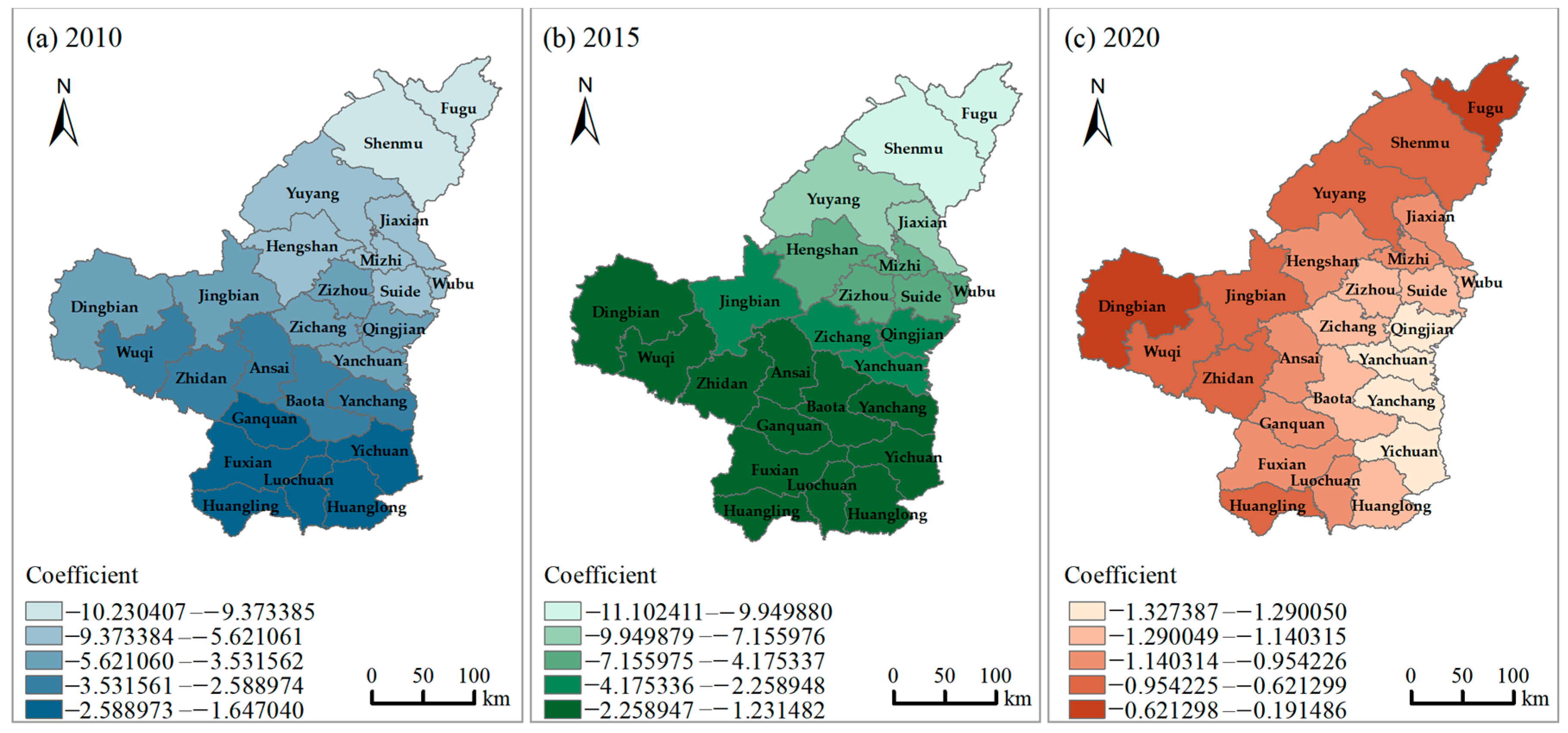
Per Capita GDP is an important parameter to measure the development degree of a region. The rise in prices and the massive consumption of water resources brought about by economic development will lead to an increase in WESV. Meanwhile, WESV will greatly decreased because of the ecological degradation caused by development, that is, the reduction in water area. Therefore, the relationship between water conservation and economic development should be balanced. The effect of per capita GDP on ESV was confirmed by Song F. [61] in a study on the value of wetland ecosystem services. Dai X. concluded that per capita GDP was negatively correlated with ESV in Chengdu [
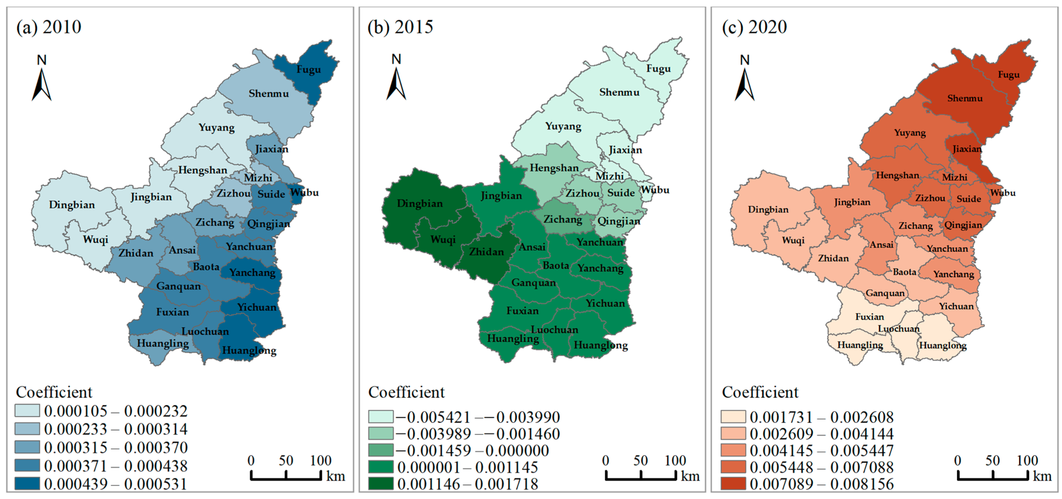
62]. As can be seen from Figure 4, per capita GDP showed time instability. The study area has undergone a process of environmental damage and recovery during a 10-year development period, which is consistent with the process in China. During 2015–2020, the construction of ecological civilization has been raised to a new level. At last, a pattern in which the degree of economic development roughly matches WESV is formed. Many studies have found that per capita GDP has an unstable impact on ESV, by influencing the level of awareness, willingness to protect the environment, and investment in environmental protection [63,64,65].
It is generally believed that the increase in population density is accompanied by the expansion of human activity areas, which will encroach on other land-use types. The water area is also experiencing depletion of rivers and lakes due to the massive depletion of surface water while the water area was occupied. Under the dual effect of the two, WESV is bound to decrease, which also explains the negative correlation between population density and WESV. It was confirmed in Chen Y.’s study of the relationship between population density and agro-ecosystem services [66]. Jiang Z. also obtained a consistent conclusion in his study of the South Four Lakes that population density was negatively correlated with Esv [67]. In recent years, the population growth rate in the study area has slowed down as in the whole country. WESV is less sensitive to population density.
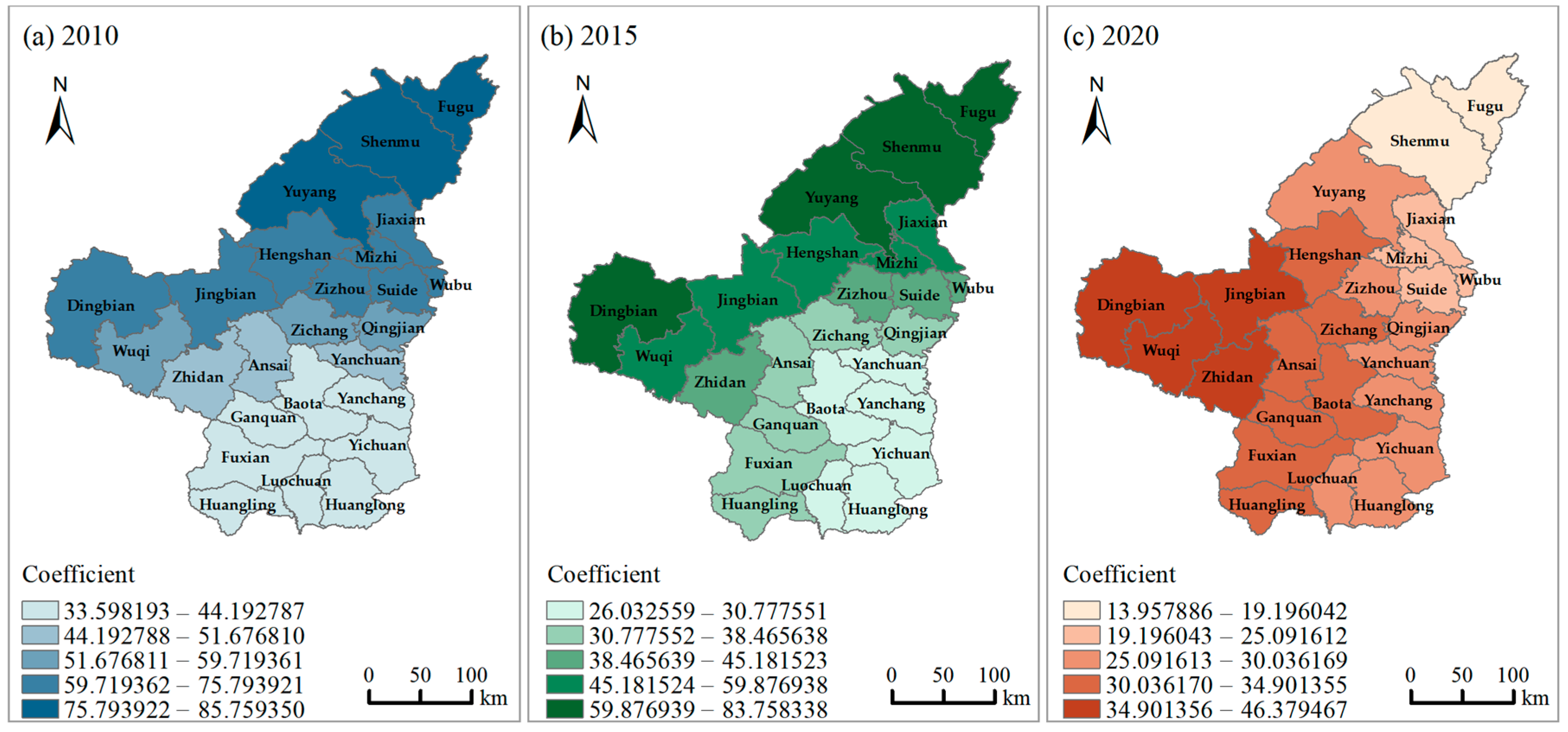
In the same region, WESV will increase with the increase in water area, which can also be explained by the calculation method adopted in this study. The equivalent factor method is to calculate the corresponding ESV according to the type of land use. Figure 6 showed that the proportion of water area has the greatest influence on WESV. During the initial stage of the study, the drier regions in the north were more sensitive. With the comprehensive management of the Mu Us Desert, the environment in the northern region has been gradually improved, and the scarcity of water resources and the vulnerability of the water environment have been alleviated. The center of influence then transferred to the west, where the pace of governance was relatively slow.
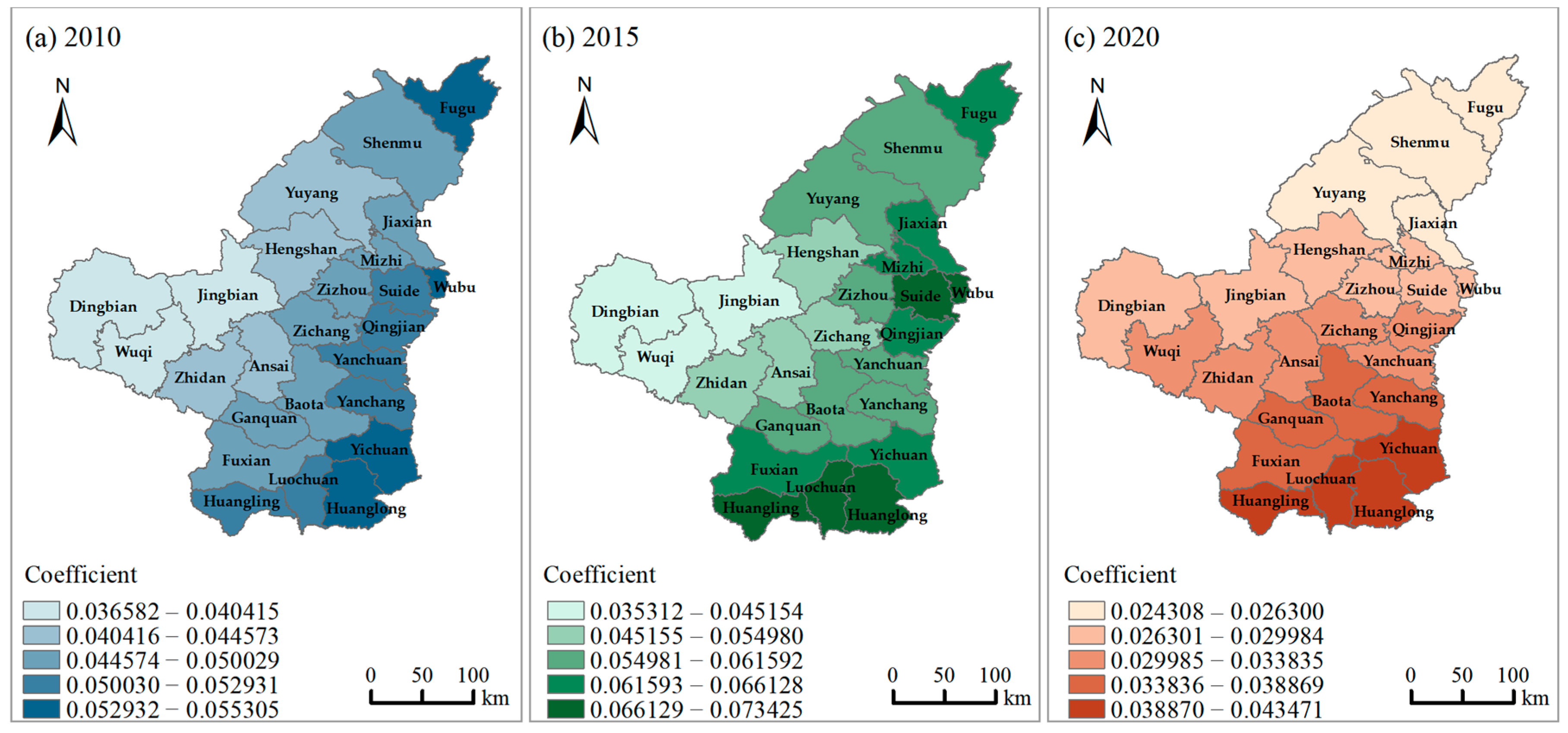
In 2010 and 2015, the impact of water consumption on WESV had a certain regularity in space, but the spatial instability that occurs cannot be ignored. Figure 7a,b can well demonstrate this phenomenon. From 2015 to 2020, the state strictly controlled the regional water consumption, and the strictest water resources management system was successfully implemented locally [68], which well explained the phenomenon that the spatial distribution pattern in 2020 was more regular.
There is spatial heterogeneity in the sensitivity of WESV to explanatory variables. Using the GWR model can more clearly show the spatial pattern of the influence degree and its evolution trend over time.

4.3. Limitations

Based on the water area obtained from remote sensing image statistics and the water consumption obtained from statistical data, this study proposed a method to quickly calculate WESV and analyze the temporal and spatial distribution of driving factors. However, the impact of water quality on WESV does not depend on water consumption or water area. Deterioration of water quality not only reduces the quality of services provided by the water resource but also incurs additional remediation costs [69]. This study did not include water quality as the basic data in the WESV assessment for three reasons. First, different types of WESVs have different sensitivity to water quality, and its mechanism of action and degree of influence are not clear, which will cause uncertainty in the calculation of WESV. Second, the equivalent factor method used in this paper is calculated from the ecological service value and the economic value of grain, and the output of grain is affected by water quality. That is to say, this study considered the impact of water quality on WESV to a certain extent. Third, the spatial and temporal scales of this study determined that water quality will not have an essential impact on WESV. In space, the county-level administrative region is the smallest research unit; in terms of time, a year is the minimum span of time. From this point of view, the water quality in the region is relatively stable, and this is also verified by the water quality data released by the environmental department. Therefore, the WESV calculated in this study is still representative and reliable without considering water quality.

5. Conclusions

In this study, taking a typical area in the central Loess Plateau as the study area, WESV was explored and assessed, and the spatiotemporal relationship between WESV and driving factors was analyzed. The conclusions obtained are as follows:
(1)
Considering surface water and groundwater as a whole, a WESV calculation method based on multi-method fusion of multiple data sources such as remote sensing images is proposed.
(2)
In total, the WESV in 2020 is 8.16% higher than that in 2010. However, during the study period, the WESV in the typical area of the central Loess Plateau experienced a process of first decreasing and then increasing. The main factor leading to this phenomenon was that the WESV of Yulin City in the north of the study area decreased by 7.84% in 2015 compared with 2010. From the perspective of the WESV composition structure, the proportion of regulating services has decreased by 18.11% in the past 10 years, but its proportion is still the largest; the proportion of provisioning services has increased year by year to 29.42%; the proportion of supporting services has decreased steadily, from 2.72% in 2010 to 2.14% in 2020.
(3)
Considering the spatial heterogeneity, the GWR model has better applicability. Among the four influencing factors, the proportion of water area and water consumption showed a positive correlation with WESV throughout the study period. Population density is negatively correlated with WESV. Per capita GDP was positively correlated with WESV in both 2010 and 2020. In 2015, there was a negative correlation between per capita GDP and WESV in the northern and western districts and counties of the study area.
(4)
With the passage of time, the spatial distribution pattern of the influence of the four factors on WESV has changed, and the evolution directions are different. The response degree of WESV to per capita GDP has evolved gradually from low in the west and high in the east to low in the southwest and high in the northeast, and the laddering nature is stronger. The water area plays a leading role in the size of WESV, and the center of gravity of the influence of the water area proportion shifts from the north to the west, with a strong decreasing law. The distribution of the influence of water consumption on WESV has experienced three evolutionary stages: small in the west and large in the east, increases in a circular shape from the west to the outside, small in the north and large in the south.

Author Contributions

Conceptualization, N.W. and Y.X.; methodology, Y.X. and N.W.; data curation, Q.W.; software, Y.X. and F.P.; validation, F.P. and Q.W.; analysis, Y.X. and N.W.; investigation, Y.X.; writing—original draft preparation, Y.X.; writing—review and editing, N.W. and Y.X.; visualization, F.P.; supervision, Q.W.; project administration, N.W.; funding acquisition, N.W. and Y.X. All authors have read and agreed to the published version of the manuscript.

Funding

This work was funded by the National Natural Science Foundation of China, Grant No. 51979221, the Natural Science Basic Research Program of Shaanxi, Program No. 2021JLM-45, and the Research Fund of the State Key Laboratory of Eco-hydraulics in Northwest Arid Region, Xi’an University of Technology, Grant No. 2019KJCXTD-5.

Institutional Review Board Statement

Not applicable.

Informed Consent Statement

Not applicable.

Data Availability Statement

Not applicable.

Acknowledgments

Sincerely, we gratefully acknowledge the State Key Laboratory of Eco-hydraulics in Northwest Arid Region, Xi’an University of Technology, for providing support. In addition, thanks to Le Zhang for her help.

Conflicts of Interest

The authors declare no conflict of interest.

References

  1. He, Y.; Wang, W.; Chen, Y.; Yan, H. Assessing spatio-temporal patterns and driving force of ecosystem service value in the main urban area of Guangzhou. Sci. Rep. 2021, 11, 3027. [Google Scholar] [CrossRef] [PubMed]
  2. Ahmad, M.; Akanji, M.A.; Usman, A.R.A.; Al-Farraj, A.S.F.; Tsang, Y.F.; Al-Wabel, M.I. Turning date palm waste into carbon nanodots and nano zerovalent iron composites for excellent removal of methylthioninium chloride from water. Sci. Rep. 2020, 10, 16125. [Google Scholar] [CrossRef] [PubMed]
  3. Costanza, R.; d’Arge, R.; de Groot, R.; Farber, S.; Grasso, M.; Hannon, B.; Limburg, K.; Naeem, S.; O’Neill, R.V.; Paruelo, J.; et al. The value of the world’s ecosystem services and natural capital. Nature 1997, 387, 253–260. [Google Scholar] [CrossRef]
  4. Millennium Ecosystem Assessments. Ecosystems and Human Well-Being: A Framework for Assessment; Island Press: Washington, DC, USA, 2003; pp. 50–60. [Google Scholar]
  5. Xie, G.; Lu, C.; Leng, Y.; Zheng, D.; Li, S. Ecological assets valuation of the Tibetan Plateau. J. Nat. Resour. 2003, 18, 189–196. [Google Scholar]
  6. Xie, G.; Zhang, C.; Zhang, L.; Chen, W.; Li, S. Improvement of the Evaluation Method for Ecosystem Service Value Based on Per Unit Area. J. Nat. Resour. 2015, 30, 1243–1254. [Google Scholar]
  7. Xiu, Y.; Wang, N.; Xie, J.; Ke, X. Improvement of the Ecological Protection Compensation Policy for Adjustment of Planting Structure in an Area of Groundwater Overexploitation: A Tripartite Evolutionary Game Study. Pol. J. Environ. Stud. 2022, 31, 1399–1414. [Google Scholar] [CrossRef]
  8. Talukdar, S.; Singha, P.; Shahfahad; Mahato, S.; Praveen, B.; Rahman, A. Dynamics of ecosystem services (ESs) in response to land use land cover (LU/LC) changes in the lower Gangetic plain of India. Ecol. Indic. 2020, 112, 106121. [Google Scholar] [CrossRef]
  9. Flotemersch, J.E.; Shattuck, S.M.; Aho, K.B.; Cox, C.E.; Cairns, M.R. Factors influencing social demands of aquatic ecosystems. Ecol. Soc. 2019, 24, 9. [Google Scholar] [CrossRef]
  10. Liu, Z.T.; Wu, R.; Chen, Y.X.; Fang, C.L.; Wang, S.J. Factors of ecosystem service values in a fast-developing region in China: Insights from the joint impacts of human activities and natural conditions. J. Clean. Prod. 2021, 297, 126588. [Google Scholar] [CrossRef]
  11. Liu, W.; Zhan, J.Y.; Zhao, F.; Yan, H.M.; Zhang, F.; Wei, X.Q. Impacts of urbanization-induced land-use changes on ecosystem services: A case study of the Pearl River Delta Metropolitan Region, China. Ecol. Indic. 2019, 98, 228–238. [Google Scholar] [CrossRef]
  12. Wang, J.L.; Zhou, W.Q.; Pickett, S.T.A.; Yu, W.J.; Li, W.F. A multiscale analysis of urbanization effects on ecosystem services supply in an urban megaregion. Sci. Total Environ. 2019, 662, 824–833. [Google Scholar] [CrossRef] [PubMed]
  13. Zhou, D.Y.; Tian, Y.Y.; Jiang, G.H. Spatio-temporal investigation of the interactive relationship between urbanization and ecosystem services: Case study of the Jingjinji urban agglomeration, China. Ecol. Indic. 2018, 95, 152–164. [Google Scholar] [CrossRef]
  14. Hu, S.; Chen, L.Q.; Li, L.; Wang, B.Y.; Yuan, L.N.; Cheng, L.; Yu, Z.Q.; Zhang, T. Spatiotemporal Dynamics of Ecosystem Service Value Determined by Land-Use Changes in the Urbanization of Anhui Province, China. Int. J. Environ. Res. Public Health 2019, 16, 5104. [Google Scholar] [CrossRef] [PubMed]
  15. Mao, Y.Y.; Hou, L.L.; Zhang, Z.D. Spatial-Temporal Evolution and Relationship between Urbanization Level and Ecosystem Service from a Dual-Scale Perspective: A Case Study of the Pearl River Delta Urban Agglomeration. Sustainability 2021, 13, 8537. [Google Scholar] [CrossRef]
  16. Peng, L.; Wang, X.X. What is the relationship between ecosystem services and urbanization? A case study of the mountainous areas in Southwest China. J. Mt. Sci. 2019, 16, 2867–2881. [Google Scholar] [CrossRef]
  17. Yang, Y.Q.; Jun, Z.; Sui, X.; He, X. Study of the spatial connection between urbanization and the ecosystem-A case study of Central Yunnan (China). PLoS ONE 2020, 15, e0238192. [Google Scholar] [CrossRef]
  18. Li, R.; Shi, Y.; Feng, C.C.; Guo, L. The spatial relationship between ecosystem service scarcity value and urbanization from the perspective of heterogeneity in typical arid and semiarid regions of China. Ecol. Indic. 2021, 132, 108299. [Google Scholar] [CrossRef]
  19. Shi, L.; Halik, U.; Mamat, Z.; Aishan, T.; Abliz, A.; Welp, M. Spatiotemporal investigation of the interactive coercing relationship between urbanization and ecosystem services in arid northwestern China. LDD 2021, 32, 4105–4120. [Google Scholar] [CrossRef]
  20. Fang, J.H.; Song, H.L.; Zhang, Y.R.; Li, Y.R.; Liu, J. Climate-dependence of ecosystem services in a nature reserve in northern China. PLoS ONE 2018, 13, e0192727. [Google Scholar] [CrossRef]
  21. Cheng, B.; Li, H.E. Impact of climate change and human activities on economic values produced by ecosystem service functions of rivers in water shortage area of Northwest China. Environ. Sci. Pollut. Res. 2020, 27, 26570–26578. [Google Scholar] [CrossRef]
  22. Watson, L.; Straatsma, M.W.; Wanders, N.; Verstegen, J.A.; de Jong, S.M.; Karssenberg, D. Global ecosystem service values in climate class transitions. Environ. Res. Lett. 2020, 15, 024008. [Google Scholar] [CrossRef]
  23. Schild, J.E.; Vermaat, J.E.; van Bodegom, P.M. Differential effects of valuation method and ecosystem type on the monetary valuation of dryland ecosystem services: A quantitative analysis. J. Arid Environ. 2018, 159, 11–21. [Google Scholar] [CrossRef]
  24. Zhao, Q.J.; Wang, Q.Y. Water Ecosystem Service Quality Evaluation and Value Assessment of Taihu Lake in China. Water 2021, 13, 618. [Google Scholar] [CrossRef]
  25. Pettinotti, L.; de Ayala, A.; Ojea, E. Benefits From Water Related Ecosystem Services in Africa and Climate Change. Ecol. Econ. 2018, 149, 294–305. [Google Scholar] [CrossRef]
  26. Li, Z.H.; Xia, J.; Deng, X.Z.; Yan, H.M. Multilevel modelling of impacts of human and natural factors on ecosystem services change in an oasis, Northwest China. Resour. Conserv. Recycl. 2021, 169, 105474. [Google Scholar] [CrossRef]
  27. Hong, Z.M.; Hao, H.; Li, C.Y.; Du, W.; Wei, L.D.; Wang, H.H. Exploration of potential risks of Hand, Foot, and Mouth Disease in Inner Mongolia Autonomous Region, China Using Geographically Weighted Regression Model. Sci. Rep. 2018, 8, 17707. [Google Scholar] [CrossRef]
  28. Cardozo, O.D.; García-Palomares, J.C.; Gutiérrez, J. Application of geographically weighted regression to the direct forecasting of transit ridership at station-level. Appl. Geogr. 2012, 34, 548–558. [Google Scholar] [CrossRef]
  29. Wu, D.C. Spatially and temporally varying relationships between ecological footprint and influencing factors in China’s provinces Using Geographically Weighted Regression (GWR). J. Clean. Prod. 2020, 261, 121089. [Google Scholar] [CrossRef]
  30. Muratoglu, A. Applications and Response Formulations of Water Footprint Methodology for Conservation of Water Resources. Ref. Module Earth Syst. Environ. Sci. 2021. [Google Scholar] [CrossRef]
  31. Muratoglu, A. Water Footprint: Concept and Methodology. Ref. Module Earth Syst. Environ. Sci. 2021. [Google Scholar] [CrossRef]
  32. Shao, Y.J.; Yuan, X.F.; Ma, C.Q.; Ma, R.F.; Ren, Z.X. Quantifying the Spatial Association between Land Use Change and Ecosystem Services Value: A Case Study in Xi’an, China. Sustainability 2020, 12, 4449. [Google Scholar] [CrossRef]
  33. Dahal, R.P.; Grala, R.K.; Gordon, J.S.; Munn, I.A.; Petrolia, D.R. Geospatial Heterogeneity in Monetary Value of Proximity to Waterfront Ecosystem Services in the Gulf of Mexico. Water 2021, 13, 2401. [Google Scholar] [CrossRef]
  34. Ren, Y.; Lü, Y.; Fu, B.; Comber, A.; Li, T.; Hu, J. Driving Factors of Land Change in China’s Loess Plateau: Quantification Using Geographically Weighted Regression and Management Implications. Remote Sens. 2020, 12, 453. [Google Scholar] [CrossRef]
  35. Wang, Y.; Wu, G.; Deng, L.; Tang, Z.; Wang, K.; Sun, W.; Shangguan, Z. Prediction of aboveground grassland biomass on the Loess Plateau, China, using a random forest algorithm. Sci. Rep. 2017, 7, 6940. [Google Scholar] [CrossRef]
  36. Zhao, G.J.; Mu, X.M.; Wen, Z.M.; Wang, F.; Gao, P. Soil erosion, conservation, and eco-environment changes in the loess plateau of china. LDD Land Degrad. Dev. 2013, 24, 499–510. [Google Scholar] [CrossRef]
  37. Fu, B.J.; Wang, S.; Liu, Y.; Liu, J.B.; Liang, W.; Miao, C.Y. Hydrogeomorphic Ecosystem Responses to Natural and Anthropogenic Changes in the Loess Plateau of China. Annu. Rev. Earth Planet. Sci. 2017, 45, 223–243. [Google Scholar] [CrossRef]
  38. Chen, J.; Yang, X.; Yin, S.; Wu, K.; Deng, M.; Wen, X. The vulnerability evolution and simulation of social-ecological systems in a semi-arid area: A case study of Yulin City, China. J. Geogr. Sci. 2018, 28, 152–174. [Google Scholar] [CrossRef]
  39. Luo, M.; Li, T. Spatial and temporal analysis of landscape ecological quality in Yulin. Environ. Technol. Innov. 2021, 23, 101700. [Google Scholar] [CrossRef]
  40. Zhang, D.; Jia, Q.; Wang, P.; Zhang, J.; Hou, X.; Li, X.; Li, W. Analysis of spatial variability in factors contributing to vegetation restoration in Yan’an, China. Ecol. Indic. 2020, 113, 106278. [Google Scholar] [CrossRef]
  41. Han, L.; Zhu, H.; Zhao, Y.; Liu, Z. Analysis of variation in river sediment characteristics and influential factors in Yan’an City, China. Environ. Earth Sci. 2018, 77, 479. [Google Scholar] [CrossRef]
  42. Hou, K.; Li, X.; Wang, J.J.; Zhang, J. An analysis of the impact on land use and ecological vulnerability of the policy of returning farmland to forest in Yan’an, China. Environ. Sci. Pollut. Res. 2016, 23, 4670–4680. [Google Scholar] [CrossRef] [PubMed]
  43. Xie, G.; Zhang, C.; Zhen, L.; Zhang, L. Dynamic changes in the value of China’s ecosystem services. Ecosyst. Serv. 2017, 26, 146–154. [Google Scholar] [CrossRef]
  44. Seidl, C.; Wheeler, S.A.; Zuo, A. High turbidity: Water valuation and accounting in the Murray-Darling Basin. Agric. Water Manag. 2020, 230, 105929. [Google Scholar] [CrossRef]
  45. Shaanxi Provincial Bureau of Statistics. Shaanxi Statistical Yearbook 2010; China Statistics Press: Beijing, China, 2010.
  46. Shaanxi Provincial Bureau of Statistics. Shaanxi Statistical Yearbook 2015; China Statistics Press: Beijing, China, 2015.
  47. Shaanxi Provincial Bureau of Statistics. Shaanxi Statistical Yearbook 2019; China Statistics Press: Beijing, China, 2019.
  48. Shaanxi Provincial Bureau of Statistics. Shaanxi Statistical Yearbook 2020; China Statistics Press: Beijing, China, 2020.
  49. Ma, Q.; Li, Y.; Xu, L. Identification of green infrastructure networks based on ecosystem services in a rapidly urbanizing area. J. Clean. Prod. 2021, 300, 126945. [Google Scholar] [CrossRef]
  50. Price Department of National Development and Reform Commission. Compilation of National Agricultural Product Cost-Benefit Data 2011; China Statistics Press: Beijing, China, 2011.
  51. Price Department of National Development and Reform Commission. Compilation of National Agricultural Product Cost-Benefit Data 2016; China Statistics Press: Beijing, China, 2016.
  52. Price Department of National Development and Reform Commission. Compilation of National Agricultural Product Cost-Benefit Data 2020; China Statistics Press: Beijing, China, 2020.
  53. Tobler, W.R. A Computer Movie Simulating Urban Growth in the Detroit Region. Econ. Geogr. 1970, 46, 234–240. [Google Scholar] [CrossRef]
  54. Russ, T.C.; Batty, G.D.; Hearnshaw, G.F.; Fenton, C.; Starr, J.M. Geographical variation in dementia: Systematic review with meta-analysis. Int. J. Epidemiol. 2012, 41, 1012–1032. [Google Scholar] [CrossRef] [PubMed]
  55. Fotheringham, A.S.; Charlton, M.; Brunsdon, C. The geography of parameter space: An investigation of spatial non-stationarity. Int. J. Geogr. Inf. Sci. Syst. 1996, 10, 605–627. [Google Scholar] [CrossRef]
  56. Pourmohammadi, P.; Strager, M.P.; Dougherty, M.J.; Adjeroh, D.A. Analysis of Land Development Drivers Using Geographically Weighted Ridge Regression. Remote Sens. 2021, 13, 1307. [Google Scholar] [CrossRef]
  57. Oshan, T.M.; Smith, J.P.; Fotheringham, A.S. Targeting the spatial context of obesity determinants via multiscale geographically weighted regression. Int. J. Health Geogr. 2020, 19, 11. [Google Scholar] [CrossRef]
  58. Wang, M.; He, G.; Zhang, Z.; Wang, G.; Zhang, Z.; Cao, X.; Wu, Z.; Liu, X. Comparison of Spatial Interpolation and Regression Analysis Models for an Estimation of Monthly Near Surface Air Temperature in China. Remote Sens. 2017, 9, 1278. [Google Scholar] [CrossRef]
  59. Wu, Z.N.; Di, D.Y.; Lv, C.M.; Guo, X.; Wang, H.L. Defining and evaluating the social value of regional water resources in terms of emergy. Water Policy 2019, 21, 73–90. [Google Scholar] [CrossRef]
  60. Chen, J.F.; Wang, Q.; Li, Q. A Quantitative Assessment on Ecological Compensation Based on Water Resources Value Accounting: A Case Study of Water Source Area of the Middle Route of South-To-North Water Transfer Project in China. Front. Environ. Sci. 2022, 10, 854150. [Google Scholar] [CrossRef]
  61. Song, F.; Su, F.; Mi, C.; Sun, D. Analysis of driving forces on wetland ecosystem services value change: A case in Northeast China. Sci. Total Environ. 2021, 751, 141778. [Google Scholar] [CrossRef] [PubMed]
  62. Dai, X.; Johnson, B.A.; Luo, P.; Yang, K.; Dong, L.; Wang, Q.; Liu, C.; Li, N.; Lu, H.; Ma, L.; et al. Estimation of Urban Ecosystem Services Value: A Case Study of Chengdu, Southwestern China. Remote Sens. 2021, 13, 207. [Google Scholar] [CrossRef]
  63. Wang, E.; Kang, N. Does life satisfaction matter for pro-environmental behavior? Empirical evidence from China General Social Survey. Qual. Quant. 2019, 53, 449–469. [Google Scholar] [CrossRef]
  64. Carrasco, L.R.; Nghiem, T.P.L.; Sunderland, T.; Koh, L.P. Economic valuation of ecosystem services fails to capture biodiversity value of tropical forests. Biol. Conserv. 2014, 178, 163–170. [Google Scholar] [CrossRef]
  65. Kang, N.; Hou, L.; Huang, J.; Liu, H. Ecosystem services valuation in China: A meta-analysis. Sci. Total Environ. 2022, 809, 151122. [Google Scholar] [CrossRef]
  66. Chen, Y.J.; Yu, Z.R.; Li, X.D.; Li, P.Y. How agricultural multiple ecosystem services respond to socioeconomic factors in Mengyin County, China. Sci. Total Environ. 2018, 630, 1003–1015. [Google Scholar] [CrossRef]
  67. Jiang, Z.; Sun, X.; Liu, F.; Shan, R.; Zhang, W. Spatio-temporal variation of land use and ecosystem service values and their impact factors in an urbanized agricultural basin since the reform and opening of China. Environ. Monit. Assess. 2019, 191, 739. [Google Scholar] [CrossRef]
  68. He, Y.H.; Wang, Z.R. Water-land resource carrying capacity in China: Changing trends, main driving forces, and implications. J. Clean. Prod. 2022, 331, 130003. [Google Scholar] [CrossRef]
  69. Keeler, B.L.; Polasky, S.; Brauman, K.A.; Johnson, K.A.; Finlay, J.C.; O’Neill, A.; Kovacs, K.; Dalzell, B. Linking water quality and well-being for improved assessment and valuation of ecosystem services. Proc. Natl. Acad. Sci. USA 2012, 109, 18619–18624. [Google Scholar] [CrossRef] [PubMed]
Figure 1. Location and administrative division of the study area: (a) Loess Plateau location; (b) study area location; (c) administrative division of the study area and DEM.
Sustainability 14 07169 g001
Figure 2. Changes of WESV among the three years in different regions.
Sustainability 14 07169 g002
Figure 3. Structural changes of WESV in the typical area of the central Loess Plateau: (a) the proportion of various WESV in 2010; (b) the proportion of various WESV in 2015 and (c) the proportion of various WESV in 2020.
Sustainability 14 07169 g003
Figure 4. Temporal and spatial distribution of the impact of Per Capita GDP on WESV in different years: (a) 2010; (b) 2015; and (c) 2020.
Sustainability 14 07169 g004
Figure 5. Temporal and spatial distribution of the impact of Population Density on WESV in different years: (a) 2010; (b) 2015 and (c) 2020.
Sustainability 14 07169 g005
Figure 6. Temporal and spatial distribution of the impact of Proportion of Water Areas on WESV in different years: (a) 2010; (b) 2015 and (c) 2020.
Sustainability 14 07169 g006
Figure 7. Temporal and spatial distribution of the impact of Water Consumption on WESV in different years: (a) 2010; (b) 2015 and (c) 2020.
Sustainability 14 07169 g007
Table 1. Classification of WESV.
Categories of WESVWork ModeContentSymbol
Provisioning Services ValueDirect supplyWater supplyV1
Indirect supplyAquatic productV2
MaterialV3
Regulating Services ValueDirect regulationHydrological regulationV4
Water purificationV5
Indirect regulationClimate regulationV6
Air regulationV7
Supporting Services ValueIndirect supportSoil conservationV8
BiodiversityV9
Table 2. Equivalent coefficients of WESV, and the WESV per unit area in different years.
Provisioning ServicesRegulating ServicesSupporting SERVICES
MaterialHydrological RegulationWater PurificationClimate RegulationAir RegulationSoil ConservationBiodiversity
Equivalent coefficient (Em)0.23 1102.24 15.55 12.29 10.77 10.93 12.55 1
2010 WESV per unit area335.15148,979.938087.233336.891122.011355.163715.76
2015 WESV per unit area1055.04303.33134,834.657319.373020.061015.481226.49
2020 WESV per unit area275.92122,650.62 6657.972747.16923.721115.663059.07
1 The equivalent coefficient was quoted from Ref. [43].
Table 3. WESV of the typical area in the central Loess Plateau. unit: million CNY.
CityCounty201020152020
YulinYuyang866.281071.751386.48
Shenmu3336.852765.083237.86
Fugu1294.82900.461194.77
Hengshan589.99686.95811.72
Jingbian1086.091070.411133.69
Dingbian918.33905.371036.14
Suide264.05249.26235.08
Mizhi114.52119.55125.89
Jiaxian404.83401.90363.29
Wubu161.24147.49143.38
Qingjian340.77309.77317.19
Zizhou54.4164.3377.94
Subtotal9432.188692.3210,063.43
Yan’anBaota352.40366.65427.71
Yanchang215.76333.62302.61
Yanchuan324.42228.90233.01
Zichang92.63101.52117.77
Ansai126.53161.89152.78
Zhidan234.91251.12270.24
Wuqi281.47319.77345.85
Ganquan213.12202.37183.24
Fuxian507.99468.73542.46
Luochuan221.64221.65274.95
Yichuan96.2396.43129.86
Huanglong15.5021.0524.65
Huangling255.62280.84310.91
Subtotal2938.223054.543316.04
Total12,370.4211,746.8613,379.48
Table 4. Structural of WESV in 2010, 2015, 2020.
WESVsContent201020152020
WESVsProportionWESVsProportionWESVsProportion
Provisioning ServicesWater supply1260.9410.19%1963.99 16.72%3729.1127.87%
Aquatic production45.080.36%122.141.04%188.061.41%
Materials22.210.18%19.400.17%19.000.14%
Regulating ServicesHydrological regulation9874.5279.83%8621.8073.40%8444.7263.12%
Water Purification536.034.33%468.033.98%458.413.43%
Climate Regulation221.171.79%193.111.64%189.151.41%
Air Regulation74.370.60%64.930.55%63.600.48%
Supporting ServicesSoil Conservation89.820.73%78.430.67%76.820.57%
Biodiversity246.281.99%215.041.83%210.621.57%
Table 5. Statistical test results and the selection of influencing factors.
ClassificationInfluence FactorUnitStatistical Test Results
Social and economyPopulation104VIF > 7.5
Population densityperson/km2VIF < 7.5, significant
Urbanization rate%VIF < 7.5, no significant
Per capital GDPyuanVIF < 7.5, significant
Gross product of primary industryyuanVIF > 7.5
Water consumption104 m3VIF < 7.5, significant
Natural environmentRainfallmmVIF > 7.5
NDVI/VIF > 7.5
Forest and grass areahm2VIF > 7.5
Forest and grass coverage ratio%VIF < 7.5, no significant
Proportion of water areaVIF < 7.5, significant
Area of soil erosion controlhm2VIF < 7.5, no significant
Table 6. Statistical test of OLS and GWR in 2010, 2015, and 2020.
201020152020
OLSGWROLSGWROLSGWR
R20.7580.8560.7920.9530.8500.906
Adjusted R20.7090.7890.7510.9150.8200.865
AICc377.181373.591364.539351.095365.338362.201
Publisher’s Note: MDPI stays neutral with regard to jurisdictional claims in published maps and institutional affiliations.

