Review

Energy Return on Investment of Major Energy Carriers: Review and Harmonization

by
David J. Murphy
1,*,
Marco Raugei
2,3,
Michael Carbajales-Dale
4 and
Brenda Rubio Estrada
1
1
Environmental Studies Department, St. Lawrence University, Canton, NY 13617, USA
2
School of Engineering, Computing and Mathematics, Oxford Brookes University, Wheatley, Oxford OX33 1HX, UK
3
Center for Life Cycle Assessment, Columbia University, New York, NY 10027, USA
4
Environmental Engineering & Earth Sciences, Clemson University, Clemson, SC 29634, USA
*
Author to whom correspondence should be addressed.
Sustainability 2022, 14(12), 7098; https://doi.org/10.3390/su14127098
Submission received: 6 May 2022 / Revised: 3 June 2022 / Accepted: 8 June 2022 / Published: 9 June 2022

Abstract

:
Net energy, that is, the energy remaining after accounting for the energy “cost” of extraction and processing, is the “profit” energy used to support modern society. Energy Return on Investment (EROI) is a popular metric to assess the profitability of energy extraction processes, with EROI > 1 indicating that more energy is delivered to society than is used in the extraction process. Over the past decade, EROI analysis in particular has grown in popularity, resulting in an increase in publications in recent years. The lack of methodological consistency, however, among these papers has led to a situation where inappropriate comparisons are being made across technologies. In this paper we provide both a literature review and harmonization of EROI values to provide accurate comparisons of EROIs across both thermal fuels and electricity producing technologies. Most importantly, the authors advocate for the use of point-of-use EROIs rather than point-of-extraction EROIs as the energy “cost” of the processes to get most thermal fuels from extraction to point of use drastically lowers their EROI. The main results indicate that PV, wind and hydropower have EROIs at or above ten while the EROIs for thermal fuels vary significantly, with that for petroleum oil notably below ten.

1. Introduction

Energy is used to power natural ecosystems as well as human societies, and it is an integral part of all economic productivity. Over the course of the industrial revolution, the proliferation of the use of fossil fuels led to massive increases in physical productivity within economies, leading to wealth accumulation, technological development, population growth, and, in short, to the rise of modernity. Society is now faced with the aftermath of the past two hundred years of growth in the form of climate change, land-cover change, biodiversity loss, and other environmental woes.
The “energy transition”, that is, the transition from fossil fuels to low carbon and renewable energy sources, is viewed by many as the means by which we can maintain our technology-intensive way of life without the concomitant environmental damage imposed by the utilization of fossil fuels. There is debate, however, about whether or not renewable energy can replace the manifold functions of fossil fuels in current society. One way in which academics frame this debate is around the concept of Energy Return on Investment [1,2,3,4]. EROI is a measure of energy profitability of energy sources and technologies [5]. In general, society benefits from energy resources and technologies that are highly profitable, which provide energy to society at very little energy cost (i.e., a large proportion of net energy). On the other hand, societies that have sources of energy that have low profitability (i.e., low EROI resources) tend to be constrained in their growth potential, among other things.
The debate about whether renewable energy can provide enough net energy to society to replace fossil fuels is beset with controversy. For instance, many papers indicate that solar photovoltaic (PV) electricity has a similar or higher EROI than natural gas electricity [6,7]; yet, there are others saying the opposite, i.e., that the EROI of PV electricity is much lower [8,9]. The same occurs for other renewable energy technologies, too. The contributions that EROI can make to the framing of the energy transition are thus limited by the seeming inability to form consensus in the literature.
This controversy is not new, and a number of authors and even the International Energy Agency have called for stricter guidelines on how EROI is calculated [10,11]. More specifically, the argument has been made for EROI practitioners to adopt the more formal methodological framework established by the life cycle assessment (LCA) community [12]. Despite these calls for more methodological rigor in EROI analyses, more consistent EROI assessments still seem elusive.
This paper arises from this academic landscape: one in which the EROIs of most major technologies are still debated and one in which the methods are often inconsistent. Therefore, its goals are threefold: first, to perform a review of the literature to provide an overview of the most recent estimates of the EROI ranges for various energy technologies and energy carriers. Second, to harmonize those values so that they are comparable across technologies. Third, to provide the data and recommendations to enable other net energy researchers to harmonize future work in hopes to avoid spurious comparisons in the literature.

2. Materials and Methods

2.1. EROI Definition

The most fundamental operational definition of EROI is listed by, among others, Dale [13] as:
E R O I = G r o s s   E n e r g y   O u t p u t E n e r g y   I n v e s t m e n t s
By this formulation, the energy delivered by the technology is divided by the energy invested to make such delivery possible (the “energy investment” is defined as the energy used to harvest an energy resource from the environment and convert it into a usable energy carrier). However, this equation is often manipulated by researchers to calculate values based on both different data sources and different system boundaries and assessment goals.
One alternative operational definition of EROI entails the use of monetary values to indirectly estimate energy investments. For instance, Court and Fizaine [14] use an economic input-output framework to calculate EROI, and their equation is:
E R O I i = E o u t , i M i n , i E I i
where Min,i is the amount of money invested in global energy sector i, and EIi is the average energy intensity of energy sector i, in exajoules per 1 USD. However, not only is this a much more descriptive formulation than that provided by Equation (1), it is also a fundamentally different calculation that opens the door to potential distortions, such as those which arise due to the elasticity of the money-to-energy relationship or the fact that this value is really a measure of the power flow, i.e., energy per unit time.
However, even foregoing the use of all economic calculations and sticking to strictly physical units only as implied by Equation (1), the literature is still replete with inconsistent EROI estimates and mismatched comparisons which, over time, risk leading to a devaluation of the very concept of EROI in general. Specifically, when reviewing the literature, two main types of methodological inconsistencies emerge, as discussed in the following sections.

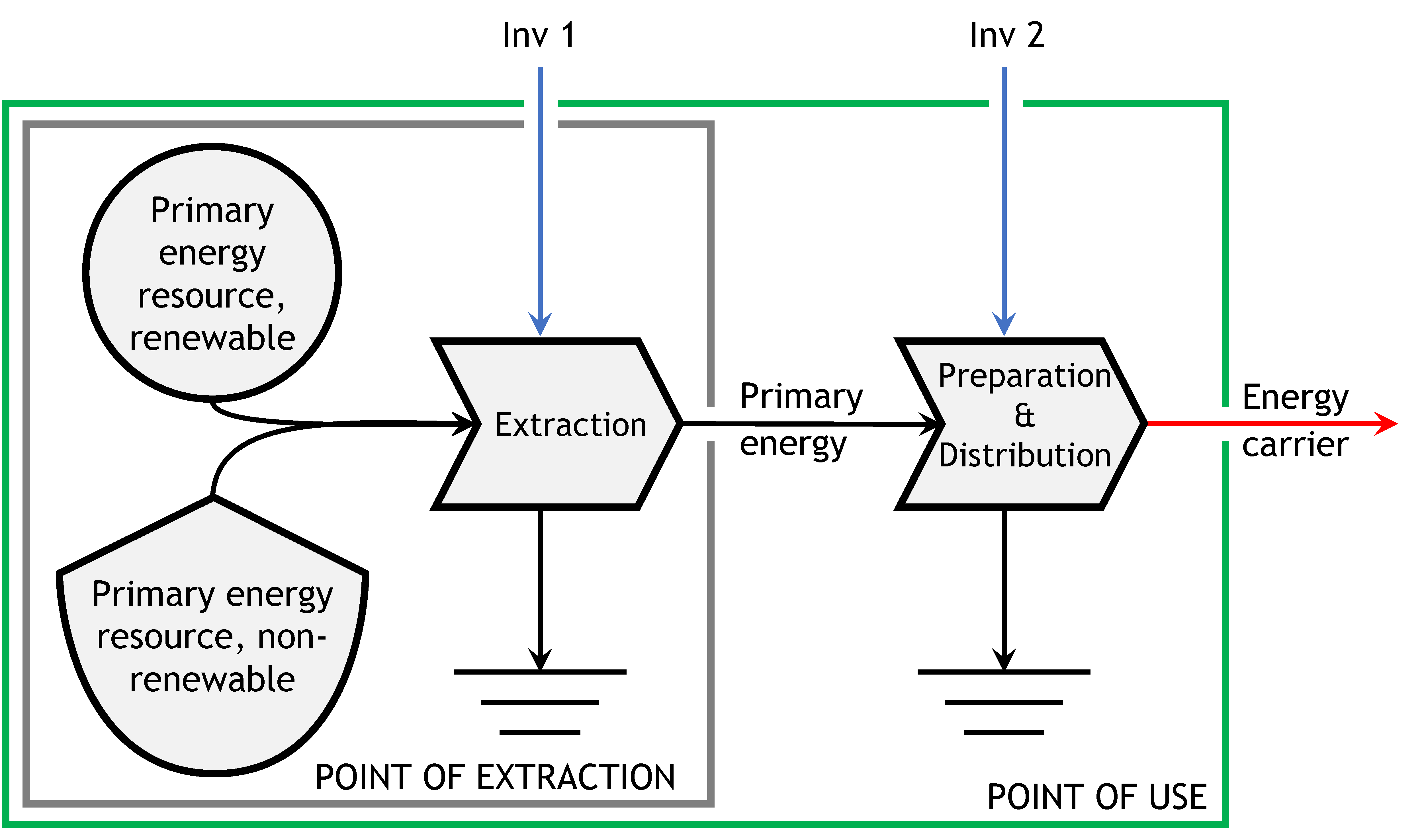
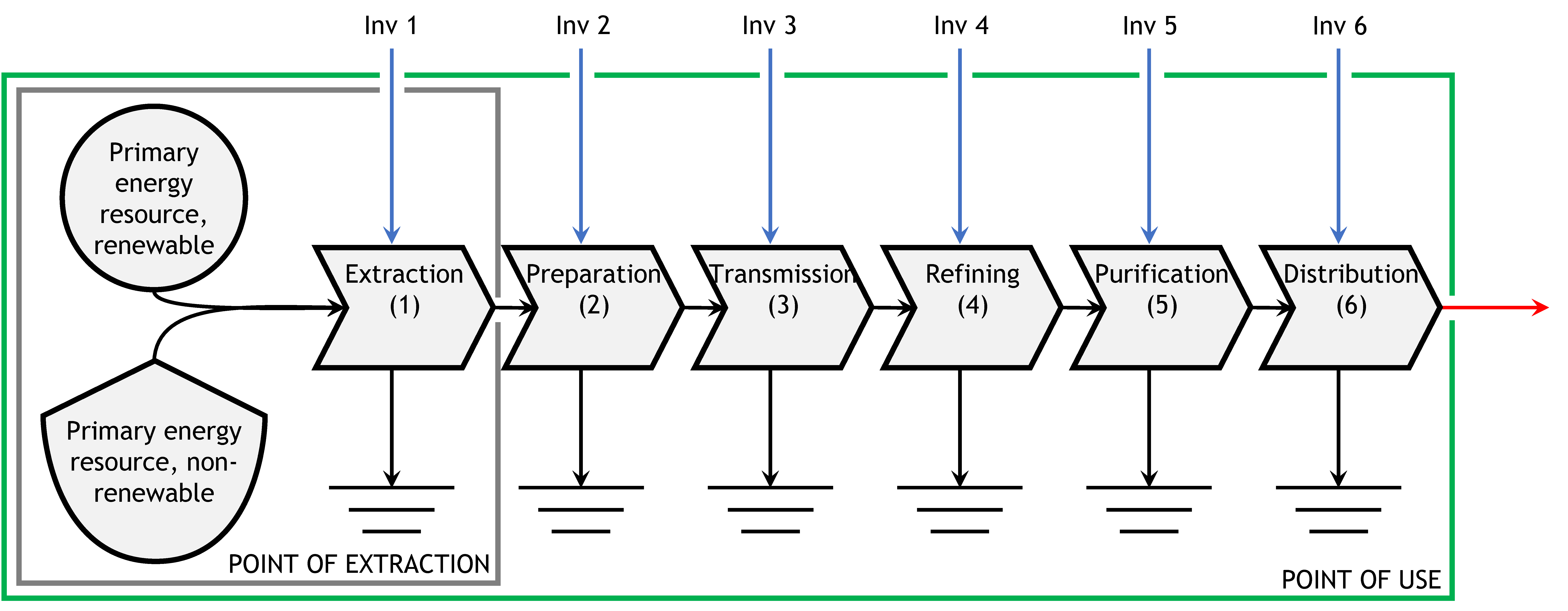
2.2. Supply Chain Boundary Mismatch

A first kind of boundary mismatch occurs whenever a comparison is made between energy carriers that are sampled at different stages of their supply chain and—most importantly—which are not functionally equivalent [15]. An extreme—but unfortunately not uncommon—example of this is when the EROI of crude oil at the well-head is compared to the EROI of electricity entering the grid [16,17].
In the most general terms possible, a primary energy resource (PES) needs to be first extracted from nature, and subsequently processed into a usable energy carrier (EC) and transported to the end user. This is illustrated schematically in Figure 1.
Much of the early EROI literature has traditionally focused on the analysis of energy resources at point of extraction [17,19], implicitly assuming that such initial stage of the supply chain would always dominate the final EROI ranking of the various types of energy that are ultimately delivered to society. However, more recently the careful analysis of a number of fossil fuel supply chains has shown that in the real world the energy investments for processing the extracted raw resources into usable energy carriers and for their subsequent transportation to the end user (i.e., Inv2 in Figure 1) are often larger than the initial energy investment for resource extraction (i.e., Inv1 in Figure 1) [15,20,21,22,23,24,25].
As the energy inputs to the EROI equation derive more and more from post-extraction processes, the comparison of “crude oil at the well head” with any downstream energy carrier, such as electricity, becomes increasingly misleading. What has become increasingly important in the recent literature is the value of energy at the point of use, after accounting for all of the energy processing inputs, since these are the energy carriers delivered to the end user to perform actual work in society.
The importance of methodological consistency is exemplified in both Table 1 and Figure 2, which report a streamlined EROI analysis of three fictional primary energy resources (PES1, 2 and 3), “at point of extraction” and “at point of use”, respectively. Given the non-linear nature of the EROI calculation (see Equation (1)), the processing energy inputs that are often excluded in fossil fuel EROIs dramatically change the resulting EROIs. For example, the PES1 has an EROI at point of extraction of 100 while the corresponding EROI for PES3 is only 25, which might lead one to conclude that PES1 is four times better than PES 3. Yet, if the same energy is assumed to be invested in the processing of all PES1, PES2, and PES3 (in this case nine units), then the EROIs at the point of use are all very similar, i.e., EROI for PES1 at point of use is 10 while that for PES3 is 7.7. In sum, an initial EROI difference at the point of extraction (i.e., a factor of four) is reduced to being only a very marginal difference at the point of use. Moeller and Murphy [26] reported similar declines in EROI from extraction to point of use, reporting a point of extraction EROI of 40 for natural gas production via hydraulic fracturing in Pennsylvania, and an EROI of 10 when that gas is delivered to the grid as electricity. Brandt [20] calculated historical EROI trends at point of extraction and point of use for domestic oil extraction in California, finding a similar trend. Additionally, Raugei and Leccisi [22] and Raugei et al. [23] traced the diminishing EROI of fossil fuels along their whole supply chains, respectively to the UK and to Chile.
Two clear take-home messages emerge from this simple exercise: (1) comparing EROI values calculated at different stages of the supply chain (i.e., EROI “at point of extraction” vs. EROI “at point of use”) is methodologically unsound and results in inconsistent “apples-to-oranges” comparisons that are devoid of any real significance; and (2) possibly even more importantly, potentially large differences in EROI values calculated “at point of extraction” can often be misleading, as necessary investments to convert the raw resources into usable energy carriers at point of use often negate large EROI differences at the “point of extraction”.

2.3. Temporal Boundary Mismatch

The second main type of inconsistency is that of temporal mismatch. Most conventional EROI analyses adopt an integrative modelling approach whereby all the energy inputs and outputs to/from the system that occur over its full life cycle are considered. Conversely, some authors have calculated “EROI” values using a different methodology, using the energy inputs and outputs for an energy system for one year. The two calculation approaches produce only marginally different results for those energy systems where the energy investment (i.e., the denominator of the EROI ratio) is almost synchronous with the energy return (i.e., the numerator). For instance, the exploitation of fossil fuel resources requires energy investments for extraction, refining and delivery of the fuels throughout the entire life of the resources. Conversely, most major renewable energy technologies, such as PV and wind, mostly only require energy investments in construction, and then entail very low to negligible additional energy investments throughout the remaining stages of the life of the technology. In this latter case, the two calculation approaches lead to very different EROI results. For instance, an “EROI” ratio calculated for the first year of PV or wind will often be very low, which can be misleading if inconsistently compared to other EROIs calculated using the more conventional integrative approach. Of course, the “EROI” of a PV system calculated as the ratio of the electricity produced during the second year of operation to the sole maintenance energy investment taking place in that same year would then be extremely large, and likewise misleading, but for some reason this latter type of calculation is rarely, if ever, encountered in the literature.
In order to avoid the ambiguity that may arise from the use of the same acronym “EROI” for what are essentially two different metrics calculated using different temporal boundaries, many authors have argued, as we do here, that when “EROI” is calculated relative to only one year of operation, it should more accurately be referred to as Power Return On Investment (PROI), because it in fact measures the ratio of two power flows (i.e., flows of energy per year) [12,13,27]. Despite such attempts at more rigorous definitions, however, a number of recent influential works still conflate EROI with PROI (Brockway et al. [28] and Court and Fizaine [2]).

2.4. Focusing on Net Energy and the “Cliff”

Net energy is defined as:
N e t   E n e r g y = G r o s s   E n e r g y   O u t p u t E n e r g y   I n v e s t m e n t s
Combining Equation (3) with Equation (1), one obtains that the mathematical relation between EROI and net energy is:
N e t   E n e r g y = G r o s s   E n e r g y   O u t p u t   1 1 E R O I
N T G = N e t   E n e r g y G r o s s   E n e r g y   O u t p u t =   1 1 E R O I
Using Equation (5), the net-to-gross energy ratio (NTG) can be plotted against EROI, resulting in the “net energy cliff” [29]—see Figure 3. Many authors have acknowledged the importance of analyzing EROIs with respect to the net energy cliff by providing figures that position EROI values on the cliff itself [15,22,28,29].
The relation of EROI and net energy is highly non-linear: an energy acquisition process that has an EROI of 1 delivers 0% net energy, while one with an EROI of 2 already delivers 50% net energy, and so forth. At the other end of the scale, a technology that extracts energy with an EROI of 10 will deliver 90% of its energy as net energy to society, and beyond that any further increases in EROI will only produce comparatively marginal improvements in the amount of net energy. In practical terms, what this means is that one needs to spend much less time worrying about whether an EROI is 20, 30, 40 or even higher, but rather simply assess whether or not it meets a given minimum acceptable EROI threshold.
There is considerable debate, of course, about what the threshold for “minimum acceptable EROI” actually is. Authors have tried estimating the minimum EROI that will provide enough net energy to sustain a modern society [1,2,3]. Not surprisingly, given the nature of the net energy cliff, the “minimum EROIs” postulated in the literature generally range from 3–10; in other words, the minimum EROI values are located along the portion of the net energy cliff curve where the net energy delivered increases rapidly with EROI. However, it should be acknowledged that setting any specific benchmark value for such ‘minimum’ EROI is intrinsically fraught with difficulties.
Firstly, from a methodological point of view, the devil is in the details, and it has been convincingly argued that the definitions of net energy given by Equations (3) and (4) are only rigorously applicable if both the gross energy output and the energy investments are measured by the same standard [30]. In other words, since the energy investments are typically accounted for in terms of primary energy (i.e., in units of “oil equivalent”), the gross energy output should also be measured in units of equivalent primary energy, if the former are to be subtracted from the latter. For clarity, one can use the subscript “PE-eq” to specify when this is done, i.e., (Gross Energy Output)PE-eq.
The most rigorous way to quantify such “primary energy equivalency” is to adopt the replacement logic that is prevalent in LCA, whereby each unit of the output energy carrier is assumed to be equivalent to X units of primary energy, where (1/X) is the overall energy efficiency of the “average” supply chain of the energy carrier in question [11,31].
Such distinction was rarely made in the early EROI literature, which tended to focus primarily on fossil fuels. Admittedly, for thermal fuel products like crude oil or coal, and even refined oil fuels and gases, the (1/X) ratio is often sufficiently close to 1 to render the numerical distinction between (Gross Energy Output) and (Gross Energy Output)PE-eq inconsequential, in light of the inevitable uncertainties that these life-cycle calculations entail. In fact, the global average value of (1/X) for all fossil fuels combined (oil + coal + gas) can be estimated to be 0.96, by using the information in the latest IEA World balance Sankey diagram [32].
Given the negligible effect that such methodologically rigorous “primary energy equivalency” calculations would have on the numerical estimate of the EROI values for thermal fuels at point of use (including also for all biofuels, which are functionally equivalent to the corresponding refined fossil fuels that they are intended to replace), in the remainder of this article all such EROI values are simply calculated as the straight ratio of the gross energy output in the fuel itself to the energy investments (i.e., as per Equation (1)).
However, when instead the Gross Energy Output is provided in the form of a highly processed energy carrier for which the average supply chain entails significant thermodynamic losses (such as is the case for electricity, when the average grid mix comprises thermal power plants, as it almost invariably does), (1/X) may be significantly lower than 1 (e.g., it is often close to 0.3 for grid mixes dominated by coal and gas electricity).
For the specific case of electricity, therefore, in the recent literature an alternative definition of EROI has emerged (Equation (6)), which makes the distinction between (Gross Energy Output) and (Gross Energy Output)PE-eq explicit [10,11]:
E R O I P E e q = G r o s s   E l e c t r i c i t y   O u t p u t P E e q E n e r g y   I n v e s t m e n t s = G r o s s   E l e c t r i c i t y   O u t p u t / η G E n e r g y   I n v e s t m e n t s
where ηG is the life-cycle efficiency of the grid mix.
Of course, the logical corollary to the argument made above, about the need to calculate Net Energy in terms of primary energy equivalents, is that whenever any EROI value for electricity is discussed in relation to the concept of net energy, and more specifically when such value is positioned on the “net energy cliff”, such EROI value should always be calculated according to Equation (6) [22,33,34].
In the remainder of this article, then, all EROI values for electricity will be harmonized to EROIPE-eq calculated according to Equation (6) above, and subject to a sensitivity analysis on the value of ηG (which may vary significantly depending on the proportion of thermal vs. renewable energy resources used to generate electricity).
One methodological complication of the alternative definition of the EROI of electricity as given in Equation (6) is that it is no longer an absolute indicator of the energy performance of the technology being analyzed, but instead it becomes a relative indicator of its performance vs. that of the average grid mix into which it is assumed to be embedded. This has important implications also in terms of how the resulting EROIPE-eq trends over time are to be interpreted, as discussed in some of the literature [34,35,36]. In simple terms, the value EROIPE-eq becomes closer and closer to the “straight” EROI (calculated as the ratio of the output electricity to the investments), as the primary-to-electric energy conversion efficiency of the grid mix as a whole improves. This is consistent with the replacement logic that underpins the definition of “primary energy equivalent”; in fact, asymptotically, if a grid mix achieved ηG = 1, then one unit of electricity would become equivalent to one unit of primary energy.
A closely related important consideration, though, is that any assumed minimum EROI threshold always implicitly rests on an assumed average efficiency for the down-stream processes in which the various energy carriers are used. Historically, the most commonly used energy carriers have been thermal fuels, whose conversion into useful work is severely constrained by the Carnot ratio (ηmax = 1 − TC/TH). However, in the coming decades, “a massive cross-sector electrification and a concomitant shift away from thermal processes […] may open the door to achieving the required services with much lower demand for primary energy, which in turn entails that a significantly lower EROI than previously assumed may suffice” [37]. In other words, all else being equal, the reduced reliance on thermal power plants in electricity grids will tend to increase ηG, and therefore decrease the EROIPE-eq of electricity, but at the same time, the resulting lower EROIPE-eq will still suffice to clear the correspondingly reduced “minimum EROI” threshold required for the support of an increasingly electrified society.

2.5. Literature Review

The literature review targeted five major academic databases: Science Direct, SCOPUS, Springer, JSTOR, and Google Scholar. The search was restricted to the years 2017 to 2020 with the twin intent to capture the latest trends in terms of which energy technologies attract the most attention, and to exclude potentially obsolete results for those technologies that are still undergoing rapid development. The search keywords used were: Energy Return on Investment, EROI, Net Energy, and Net Energy Return Ratio. Overall, the search returned 113 papers in total. Each returned paper was added to a master database in Microsoft Excel that recorded the full bibliographic information, the resource type being analyzed, and the published EROI for each energy resource type. A manual screening process was then employed to discard those papers which did not report original EROI values or which were found to be critically lacking in transparency; more detail about the results of the screening process are given in Section 3.1. One exception to this search was made, and that is the inclusion of Leccisi and Fthenakis [36], which was published in 2021 and was included to represent the most recent values for PV, given the extremely rapid pace of development for this technology.

2.5.1. Literature on EROI of Thermal Fuels

There are a range of resources and products in the oil industry, so to limit spurious comparisons, this review was limited to conventional and shale oil production, inclusive of both on-shore and off-shore production [23,38,39,40,41,42,43,44,45,46]. Studies that calculated oil and gas EROI together were excluded since the individual values could not be separated, e.g., Brockway et al. [28]. EROI estimates for oil sands operations were also included; it is noteworthy that these represent a fundamentally different resource base and production process [47].
Ten papers made estimates of the EROI of natural gas. Estimates from both conventional and shale gas were included in this analysis [14,27,28,39,41,42,43,46,48,49].
Data collected for coal EROI estimates come from nine papers, which include estimates for both coal at point of extraction and coal-fired electricity generation [14,22,27,28,39,44,46,48,49,50]. Other papers analyze coal seam gas and coal-to-liquids technologies [43,51].
The literature on the EROI of biodiesel includes seven papers with estimates for different feedstocks, including jojoba [52]; waste cooking oil [53,54]; soybean, palm, microalgae, soybean, animal fat, palm oil [55]; African palm, pinion, bovine and swine fat [56]; photoautotrophic algae, hybrid biofuel [57]; and agroforestry and first-generation soybean with and without co-products [58]. Three different papers presented EROI estimates for bioethanol. Different feedstocks for the production of bioethanol include sugarcane, corn, wood [56]; almond shells [59]; and corn grain [55]. One paper provided EROI estimates for biogas [60], and one for wood chips [23].

2.5.2. Literature on EROI of Electricity

Three research papers included EROI estimates from pressurized water nuclear reactors [46,49,50].
The literature search returned three papers with estimates for the EROI of bioenergy with carbon capture and sequestration (BECCS) systems. The feedstocks used in the papers analyzed herein include microalgae, biodegradable waste, lignocellulosic biomass, wheat, switchgrass, miscanthus, and willow [61,62,63].
There were four estimates of the EROI of geothermal energy sources from four separate analyses. These analyses were limited to geothermal systems that produce electricity, and do not include ground-source heat pump systems which are an often confused with the former, but are an altogether different technology [46,48,49,50].
There were five papers that made estimates of the EROI of hydropower. Literature collected included only conventional dam and run-of-river hydropower production, and excluded oceanic power and hydrothermal liquefaction [46,48,49,50,64].
Eight papers estimated EROI values for solar PVs, encompassing mono-silicon, poly-silicon, cadmium-telluride (CdTe), and copper indium gallium di-selenide (CIGS) [34,36,46,49,50,65,66,67]. Estimates for perovskite PVs were excluded since these technologies are not yet commercially viable and much uncertainty remains on their durability.
One paper provided an EROI estimate for concentrating solar power (CSP) [35].
Ten studies made estimates of the EROI of wind power, both from conventional on-shore and off-shore wind turbines [46,49,50,64,66,68,69,70,71,72]. Smaller (<1 MW) micro-wind turbines were not analyzed.

2.6. EROI Harmonization

EROI values were often reported for each study for a number of different technologies. The first part of our harmonization process separated these energy technologies and resources into two categories: (1) thermal fuels at the point of use, and (2) electricity at the point of use. Thermal fuels at the point of use include oil fuels, natural gas, coal, biodiesel, bioethanol and biogas. Electricity at the point of use includes natural gas electricity, coal-fired electricity, nuclear electricity, biomass electricity (with and without carbon capture and sequestration), geothermal electricity, hydropower, solar photovoltaics, concentrating solar power and wind power.

2.6.1. Harmonization of EROI Values of Thermal Fuels

EROI values from the studies were made consistent with respect to the process chain boundary, as discussed above in Section 2.2. Specifically, data was taken from the life-cycle database Ecoinvent (v3.7 and v3.8) [73] to provide information on inputs to all the individual supply chain processes that follow resource extraction (namely: preparation, transmission, refining, purification, and distribution), as depicted in Figure 4 below. For the specific case of oil-derived fuels, given the plurality of fuels that are simultaneously produced at the refining stage, the decision was made to focus on petrol (i.e., gasoline) as a representative case in point (energy investment allocation for refining was made on the basis of the exergy content of the output fuels, so the results essentially hold for all other co-products, too). For the coal supply chain, hard coal (as opposed to brown coal or lignite) was assumed. Additionally, given the large variability in transport distances, the associated investments for transmission and distribution were estimated on the basis of global average distances for each fuel supply chain as reported by Ecoinvent.
In Table 2, data are presented on energy investments to each of the post-extraction unit processes in Figure 4, expressed as % relative to the energy in the output fuel. Additionally, Table 2 also reports the cumulative post-extraction energy investments in the supply chain up to and including that process, and the associated maximum EROI at that point in the chain (i.e., the EROI that would result at that point of the chain as a consequence of the post-extraction energy investments only, even assuming an initial infinite EROI at point of extraction). These data were used to harmonize results from studies that presented EROI results at different points in the chain by adding in information from ‘missing’ processes up to the point of use (POU). More detailed information with full calculations and links to specific datasets from Ecoinvent can be found in the Supplementary Materials.
By including this information in the paper, any analyst in the net energy community can, for example, plug their own EROI values at point of extraction in the appropriate cell in the spreadsheet, and then quickly find a standardized value for the corresponding EROI at point of use.
Note also that, even ignoring the extraction process completely, the downstream processing chain sets an upper limit to the EROI value of the product at the point of use. For example, bioethanol from maize (corn) would have an EROI of 1.6 even without including any energy investments for crop production. This is due mainly to the enormous energy penalty (over 60%) in the refining process. This can be contrasted to the refining process for sugarcane, which requires an investment equivalent to only 2% of the energy in the fuel. Additionally, it is important to point out that, irrespective of their initial EROI at point of extraction, all conventional fuels derived from fossil resources end up having a maximum EROI at point of use well below 10. It bears reiterating that this is the sole consequence of the multiple unavoidable energy investments that are required post-extraction, along the supply chain, to convert the “raw” fossil resources (e.g., crude oil) into usable fuels at point of use (e.g., petrol or diesel at the pump, or heavy fuel oil at point of delivery). While these findings may be surprising and perhaps counterintuitive to some, they are actually in perfect alignment with a recent high-level study that used IEA data and extended multi-regional input–output tables to estimate EROI at point of use for all fossil fuels produced globally [28].

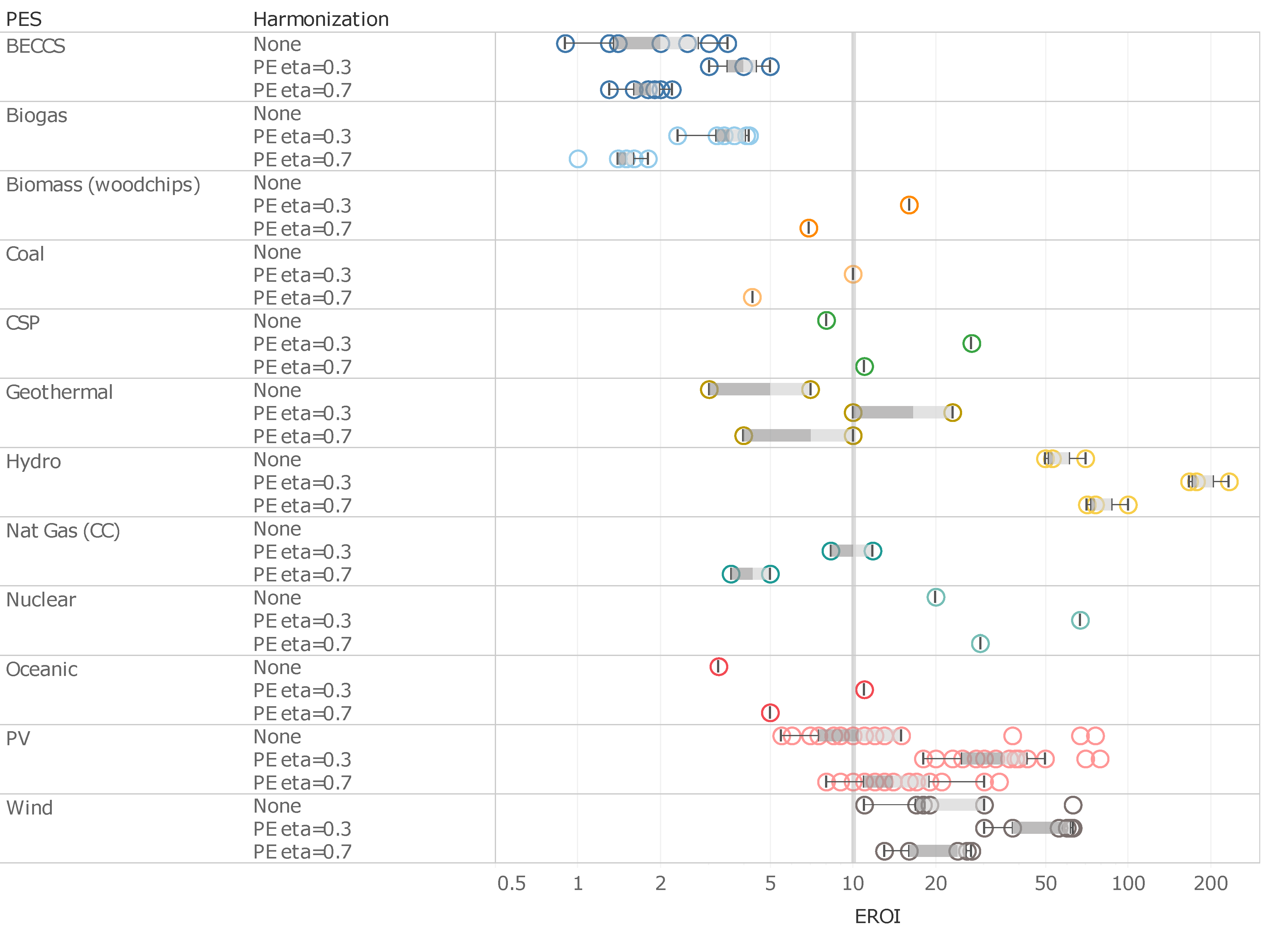
2.6.2. Harmonization of EROI Values of Electricity

As expected, the reviewed literature was inconsistent in terms of whether the reported EROI values had been calculated as “straight” ratios of electricity output to primary energy investment, or “weighted” ratios, where the electricity output at the numerator is “converted” into primary energy equivalents, based on some assumed coefficient.
In order to harmonize all the collected EROI values for electricity from nuclear, BECCS, hydro, geothermal, oceanic, PV, CSP, and wind, the following process was therefore employed:
(i)
all “straight” EROI ratios were consistently multiplied by the same fixed 1/ηG value, thereby calculating the corresponding EROIPE-eq, as per Equation (6). Given the critical sensitivity associated to ηG (as discussed in Section 2.3), a sensitivity analysis was carried out by repeating such calculation twice, first by setting ηG = 0.3 (representative of deployment in most grid mixes dominated by conventional thermal generators), and then by setting ηG = 0.7 (representative of deployment in a typical “decarbonized” grid mix with a significant penetration of renewable energies [7]).
(ii)
All “weighted” EROI ratios were first divided by whatever weighting factor had originally been assumed by the authors, thereby essentially undoing any such weighting and reverting to the corresponding “straight” EROIs where the numerator is simply the electricity output. Then, the same procedure as for (i) was applied, so as to once again arrive at two sets of EROIPE-eq values, respectively based on assumed ηG = 0.3 and ηG = 0.7 life-cycle primary-to-electricity conversion factors.
Additionally, EROI values for electricity from combustion of coal, natural gas, biogas, and biomass (wood chips) were also estimated, by leveraging the EROI values “at point of use” for the respective thermal fuels that were obtained from the previous harmonization process described in Section 2.6.1, and then multiplying those values by the respective Ecoinvent-sourced power plant heat rates (i.e., 0.34 for coal, 0.47 for gas combined cycles, 0.35 for biogas, and 0.24 for biomass). Finally, the resulting EROI values were multiplied by the same fixed 1/ηG values of 0.3 or 0.7, respectively, as described at point (i) above, to convert them to “primary energy equivalent” (EROIPE-eq). It is noted that, technically, this process fails to account for the additional energy investment for power plant construction and maintenance, but the data has shown that the latter is negligible for large thermal power plants when such investment is spread out over their long service life. For the specific case of gas-fired electricity, the more modern and efficient combined-cycle operation was assumed; additionally, the energy investment for gas distribution (stage 6 in Table 2) was omitted.

3. Results

The main results of our literature search and harmonization analysis are (in no particular order, and with detailed explanations in the following sections):
-
A total of 113 papers were found reporting EROI values, but, after screening them, the harmonization used only 31 papers.
-
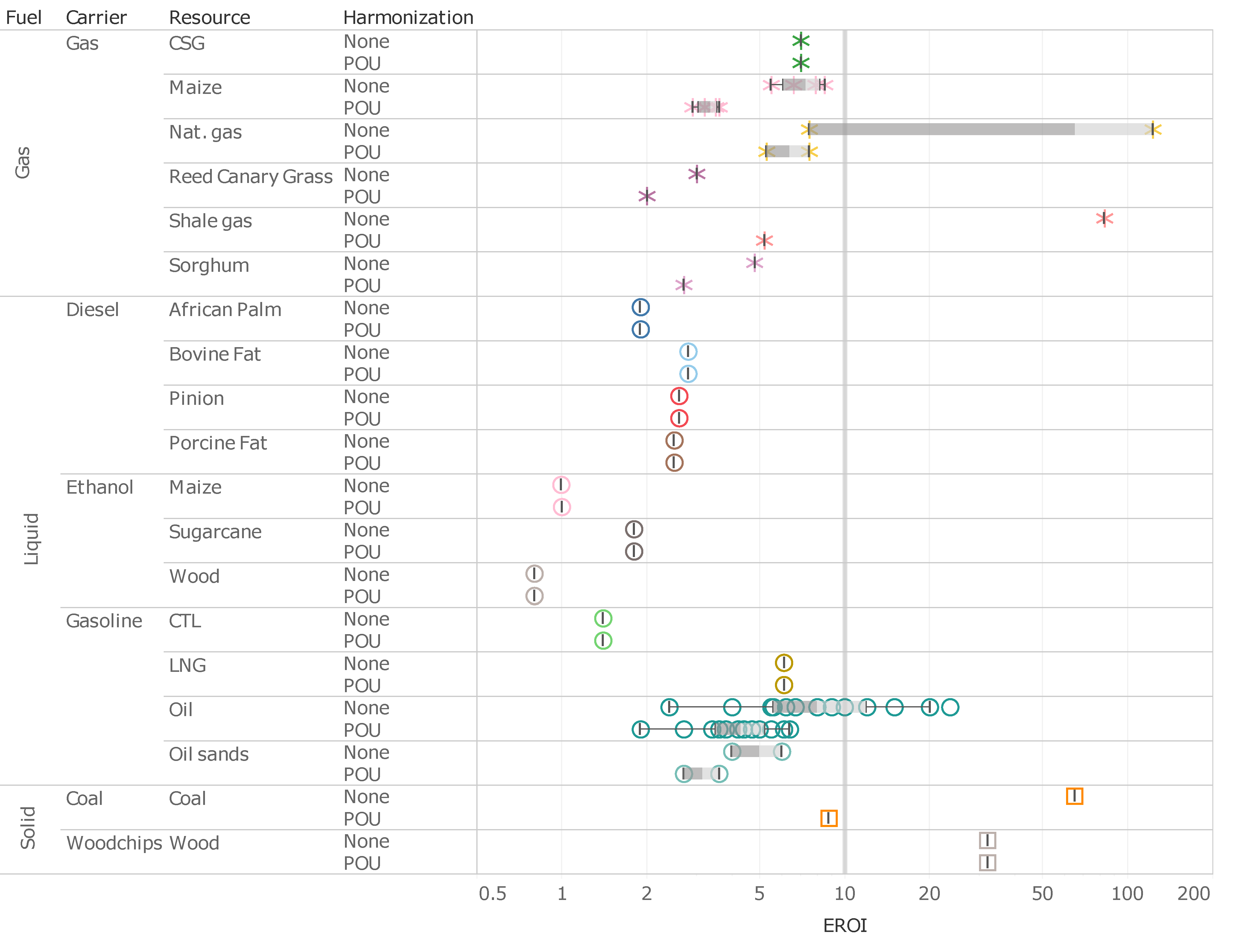
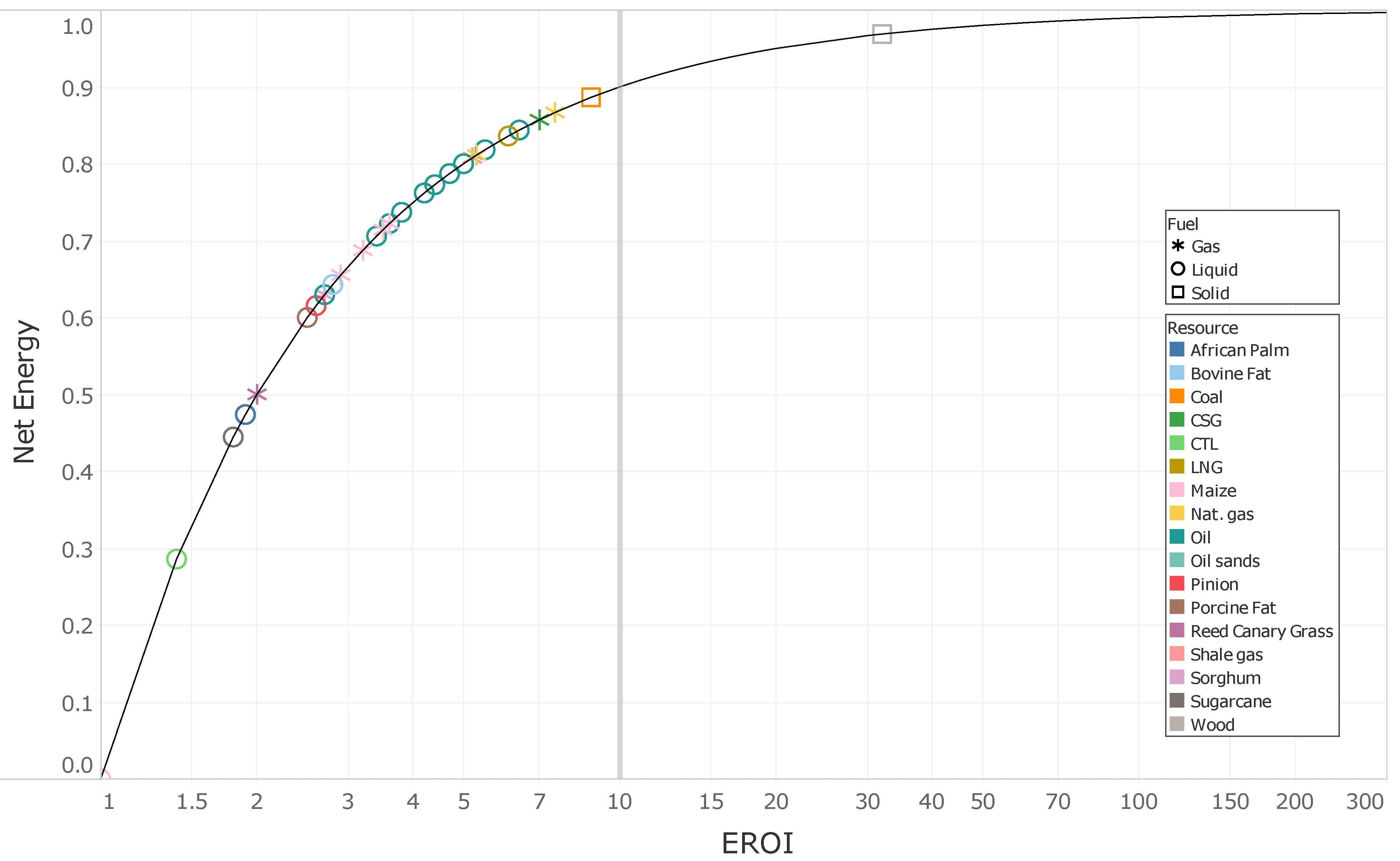
Most thermal fuels, including biofuel, oil, and natural gas have EROIs well below 10 after accounting for the entire production chain to the point-of-use.
-
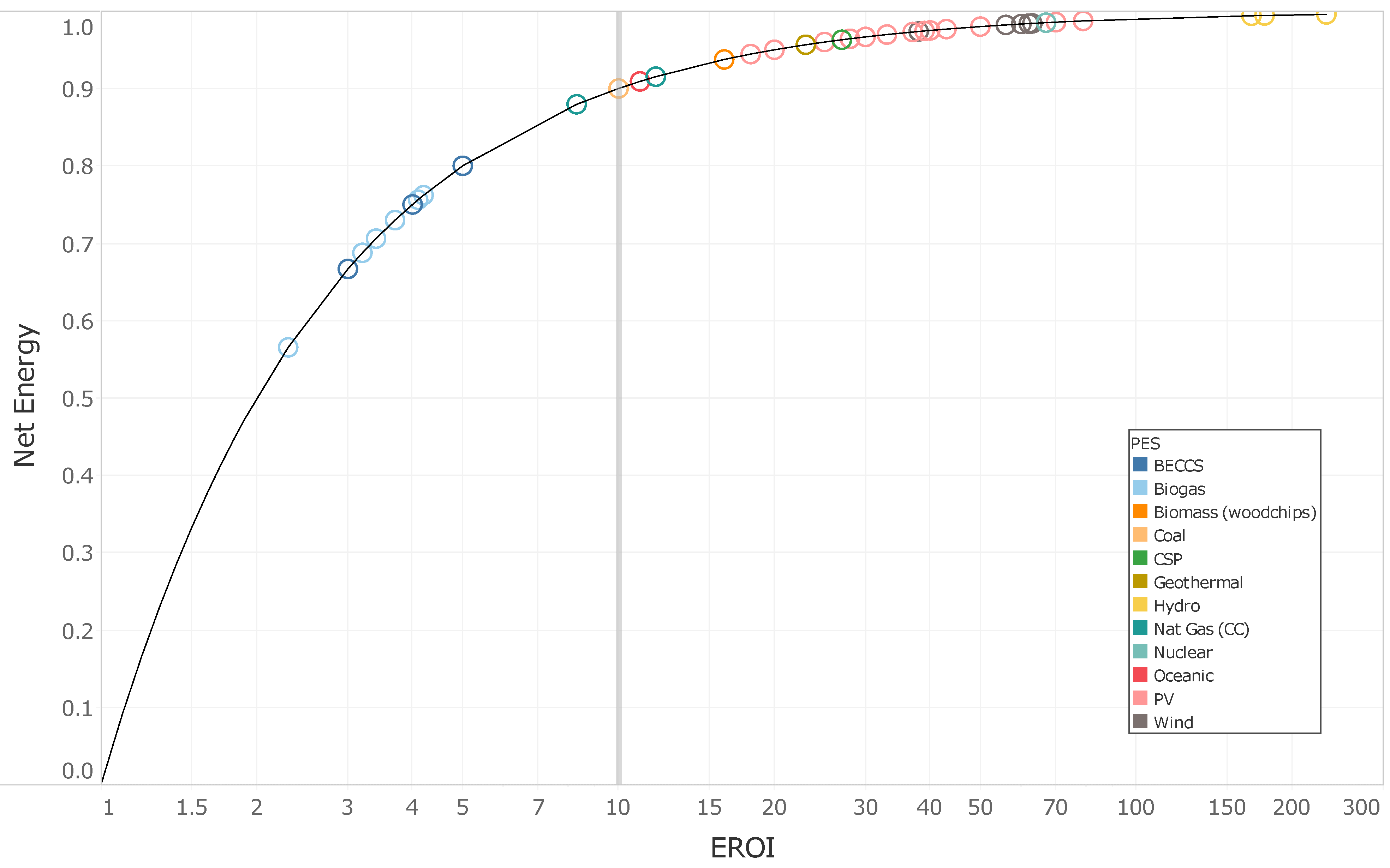
EROIs from electricity production from hydro, wind, and PV are all at or above 10, once they are consistently expressed as “primary energy equivalent” (EROIPE-eq).

3.1. Literature Screening

Out of the total 113 papers, 84 reported EROI values for the energy resources listed in Table 3. Of the remaining 29 papers, many were EROIs of technologies that fell outside the intended scope of this paper (e.g., EROI of agroecological systems). The remaining 84 EROI values were then screened to remove duplicates, i.e., EROI values that were in some way derived from previous EROI values calculated in other papers. The post-screening tally was reduced substantially to only 37 papers across all technologies (Table 3).

3.2. Harmonization Analysis

3.2.1. EROIs of Thermal Fuels at Point of Use

Using data from Table 2, EROI values from the different studies were compared on both an ‘as-is’ (harmonization = None) basis and a harmonized (Harmonization = POU) basis. These results are presented in Figure 5. Note that the horizontal axis for EROI is on a logarithmic scale. The first thing to note is that there is large variability in results, but that most of the energy products have EROI values below 10, when taken to POU. This is true of both biofuels and, importantly, also of oil, coal, and gas.
For gaseous fuels, natural gas has the highest EROI. Shale gas EROI estimates fell from 83 at point of extraction to 5.2 at POU due mainly to the large energy investments in the transmission and distribution stages. Many of the bio-based gas products suffer a large penalty (15%) in the biogas-to-biomethane purification process.
For liquid fuels, none of the conventional oil products have an EROI above 10, and together the estimates for oil have a median EROI value of 4.2 when harmonized to POU. All other estimates for bioethanol, biodiesel, and petrol from oil sands have harmonized EROIs below 5.
For solid fuels, hard coal has a harmonized EROI of 8.8. The very high value (32) for solid biomass deserves special discussion, as this is only for the specific case of locally-sourced woodchips, which entail a comparatively simple and low-energy intensive supply chain. It should, however, be noted that the EROI of solid biomass fuels varies significantly for other fuels at point of use that require more energy-intensive supply chains (e.g., the maximum EROI for wood pellets would be only 1.6, as per Table 2). As a consequence, the single value for woodchips reported here in Figure 5 and Figure 6 should not be misconstrued to be representative of the wider spectrum of solid biomass fuels.
The ‘net energy cliff’ for thermal fuels at POU is presented in Figure 6. As mentioned previously, many of the energy products have EROIs below 10, meaning that less than 90% of the net energy content in the fuel is available to society. As noted above, liquid fuels (circles) tend to have lower EROIs than solid (squares) or gaseous fuels (asterisks).

3.2.2. EROIs of Electricity at Point of Use

The results of the harmonization calculations for the EROI of electricity, described in Section 2.5.2, are reported in Figure 7. For each of the following primary energy sources (PES): nuclear, BECCS, hydro, geothermal, oceanic, PV, CSP, and wind, three values are shown, i.e., the original non-harmonized EROI (“None”), and the two harmonized ratios (“PE eta = 0.3” and “PE eta = 0.7”, respectively). For thermal electricity from coal, gas (combined cycle), biogas, and biomass (wood chips), only the harmonized EROIPE-eq ratios are reported, since these were calculated from the harmonized EROIs at point of use for the respective fuels (cf. Section 2.6.2). Methodologically consistent internal comparability is thus made possible among each of the individual sets of harmonized EROIPE-eq values.
By analyzing the obtained results, the following general observations can be made:
  • Hydroelectricity exhibits the highest EROIPE-eq results by far. The second highest-ranking group of technologies in terms of harmonized EROIPE-eq comprise: nuclear, wind, and—in some cases—PVs (see point 2. below for caveats on the latter). CSP and geothermal electricity can then be grouped together as the third “block” of results in descending order of EROIPE-eq. Broadly speaking, all electricity generation technologies listed thus far are characterized by harmonized EROIPE-eq values greater than 10, when calculated assuming a primary energy to electricity life-cycle conversion factor ηG = 0.3. Oceanic electricity straddles this symbolic EROIPE-eq = 10 line.
  • The EROIPE-eq values for PV electricity (and to a lesser extent also for geothermal electricity) span a fairly wide range. This appears to be primarily due to intrinsic differences in the assessed supply chains and technologies. Specifically, for the case of PV, the technological differences among the various technologies (sc-Si, mc-Si, CdTe and CIGS) are compounded by the large effect of variations in assumed solar irradiation (from approximately 1000 kWh·m−2·yr−1 for northern latitudes e.g., Germany, to over 2300 kWh·m−2·yr−1 for southern latitudes e.g., Chile). However, the deliberate choice was made not to attempt any harmonization for the latter, since it represents a real-world variable and not a methodological inconsistency per se. The important take-home message in these cases is that it is unreasonable to expect to arrive at a single value (or a very tight range of estimates) for the EROIPE-eq of these technologies, due to the intrinsic variability ranges that characterize them.
  • The EROIPE-eq values for thermal electricity from the combustion of fossil fuels (coal and natural gas) are both in the range of 10–12, when calculated using ηG = 0.3.
  • Thermal electricity from biogas and BECCS is characterized by comparatively low EROIPE-eq values of 2–5, when calculated using ηG = 0.3. While these results may appear to contradict some higher estimates in the previous literature, it seems likely that in those earlier studies some of the supply chain investments identified in Table 2 may have been missed. For instance, Raugei et al. [23] caveated their results for biomass- and biogas-fired electricity by stating that “EROI results for these technologies are affected by a larger margin of uncertainty, due to a combination of older inventory data and (for biomass and biogas) possible inaccuracies in the modelling of the feedstock supply chains”.
  • Finally, the calculated EROIPE-eq values for biomass-fired electricity using wood chips is comparatively high at 16 (assuming ηG = 0.3). However, as discussed in Section 3.2.1 for wood chips as a fuel stock, this result is only valid for this particular biomass fuel, whereas it would be considerably lower if a blend of woodchips and wood pellets were employed instead (as is the case in the UK, for instance [22]).
In more general terms, the systematically lower EROIPE-eq values for all technologies, when calculated using ηG = 0.7 should not surprise nor be a reason for concern. This is simply the consequence of assuming deployment in a grid mix that is itself on average significantly more efficient at converting primary energy into electricity over its whole life cycle. As discussed in Section 2.4, while the individual EROIPE-eq for all technologies would be reduced in such conditions, at the same time it is reasonable to expect that, in the future, the same widespread deployment of low-cost renewable energies that will lead to a higher ηG = 0.7 in the first place will also enable a higher degree of electrification across multiple sectors and end uses, thereby essentially lowering the “minimum EROI” threshold to above that which a healthy societal energy metabolism may be sustained.
At present, the EROIPE-eq values obtained by setting ηG = 0.3 may still be considered the more representative ones, as the use of thermal technologies to generate electricity is still prevalent globally. These values were therefore selected to be reported vs. the corresponding NTG ratios (i.e., superimposed on the “net energy cliff”) in Figure 8. This latter figure allows a clearer visualization of which electricity generation technologies can be expected to generate sufficient net energy over their life cycles. Once again, the results show that most renewable technologies actually lead to NTG > 0.9, meaning that over 90% of the equivalent primary energy returned by them remains available for societal uses other than supporting the energy sector itself. Overall, this is a reassuring result that should put to rest many often-voiced concerns about the net energy viability of non-conventional and renewable electricity.

4. Discussion and Conclusions

The analysis performed herein represents a much-needed update and harmonization of the EROI literature, and it advances the conversation surrounding the viability of renewable resources in the energy transition process. A common argument is that the EROIs from renewable energy technologies are supposedly lower than those provided by fossil fuels, and that transitioning to RE technologies would therefore result in a large loss in net energy. The results of this analysis rebuke that sentiment, noting that the three most important technologies for the energy transition—wind, PV, and hydropower—all have EROIs at or above 10 (even when the output is weighted in terms of primary energy equivalent assuming a future-proof life-cycle grid efficiency of ηG = 0.7, i.e., 1 unit of electricity per 1.4 units of primary energy). This means that greater than 90% of the energy produced by these technologies is delivered to society as net energy.
Perhaps more interesting still, the EROIs from liquid fuels, including the EROI from conventional oil production, are less than 10 once the costs of refining and delivery to the point-of-use are included. Oil is widely considered the most important fuel for the economy, used mostly in the transportation sector. This means that oil delivers less net energy to society for each unit invested in extraction, refining, and delivery than PV or wind. The transition to electric vehicles, according to these results, will actually increase the amount of net energy delivered to society (even more so when considering the higher efficiency of electrical power trains vs. internal combustion engines).
It is clear from these results that EROI estimates at the point of extraction can be wildly misleading. As a case in point, even if crude oil were measured to have an EROI of 1000 or more at the point of extraction, the corresponding EROI at the point of use, using global average data for the energy “cost” of the process chain, would still only be a maximum of 8.7. Furthermore, as the quality of oil, gas and coal continue to decline in the future, the energy “cost” of the associated process chains will increase, further reducing the EROIs. On the other hand, as the technologies used to harness renewable energy improve, the corresponding EROIs will continue to increase in the future.
Finally, it is also important to observe that, in the future, a significant increase in the penetration of renewable technologies into the electricity grid mixes will have to be accompanied by a concomitant deployment of electrical storage, to compensate for the intrinsic intermittency or renewable energy availability and ensure the continued real-time matching of the supply and demand curves. However, detailed scenario analyses of the net energy performance of even highly decarbonized grid mixes relying heavily on PVs, based on high temporal resolution grid balancing algorithms rather than blunt assumptions, indicate that the additional energy investment for electrochemical energy storage does not significantly affect the overall EROIPE-eq of the resulting electricity mix [7,11].

Supplementary Materials

The following are available online at https://www.mdpi.com/article/10.3390/su14127098/s1: “EROI_harmonization.xls”, providing detailed supply-chain energy investment calculations for selected thermal fuels, with references.

Author Contributions

Data curation, B.R.E., D.J.M., M.R. and M.C.-D.; Formal analysis, D.J.M., M.R. and M.C.-D.; Writing—original draft, D.J.M., M.R. and M.C.-D. All authors have read and agreed to the published version of the manuscript.

Funding

This research received no external funding.

Institutional Review Board Statement

Not applicable.

Informed Consent Statement

Not applicable.

Conflicts of Interest

The authors declare no conflict of interest.

References

  1. Hall, C.A.S.; Balogh, S.; Murphy, D.J.R. What Is the Minimum EROI That a Sustainable Society Must Have? Energies 2009, 2, 25–47. [Google Scholar] [CrossRef]
  2. Fizaine, F.; Court, V. Energy Expenditure, Economic Growth, and the Minimum EROI of Society. Energy Policy 2016, 95, 172–186. [Google Scholar] [CrossRef]
  3. Brandt, A.R. How Does Energy Resource Depletion Affect Prosperity? Mathematics of a Minimum Energy Return on Investment (EROI). BioPhysical Econ. Resour. Qual. 2017, 2, 2. [Google Scholar] [CrossRef] [Green Version]
  4. Lambert, J.G.; Hall, C.A.S.; Balogh, S.; Gupta, A.; Arnold, M. Energy, EROI and Quality of Life. Energy Policy 2014, 64, 153–167. [Google Scholar] [CrossRef] [Green Version]
  5. Hall, C.A.S.; Lavine, M.; Sloane, J. Efficiency of Energy Delivery Systems: Part 1 An Economic and Energy Analysis. Environ. Manag. 1979, 3, 493–504. [Google Scholar] [CrossRef]
  6. Bhandari, K.P.; Collier, J.M.; Ellingson, R.J.; Apul, D.S. Energy Payback Time (EPBT) and Energy Return on Energy Invested (EROI) of Solar Photovoltaic Systems: A Systematic Review and Meta-Analysis. Renew. Sustain. Energy Rev. 2015, 47, 133–141. [Google Scholar] [CrossRef]
  7. Raugei, M.; Peluso, A.; Leccisi, E.; Fthenakis, V. Life-Cycle Carbon Emissions and Energy Return on Investment for 80% Domestic Renewable Electricity with Battery Storage in California. Energies 2020, 13, 3934. [Google Scholar] [CrossRef]
  8. Ferroni, F.; Hopkirk, R.J. Energy Return on Energy Invested (ERoEI) for Photovoltaic Solar Systems in Regions of Moderate Insolation. Energy Policy 2016, 94, 336–344. [Google Scholar] [CrossRef] [Green Version]
  9. Prieto, P.A.; Hall, C. Spain’s Photovoltaic Revolution: The Energy Return on Investment; Springer: New York, NY, USA, 2013. [Google Scholar]
  10. Raugei, M.; Frischknecht, R.; Olson, C.; Sinha, P.; Heath, G. Methodological Guidelines on Net Energy Analysis of Photovoltaic Electricity; International Energy Agency: Paris, France, 2016. [Google Scholar]
  11. Raugei, M.; Frischknecht, R.; Olson, C.; Sinha, P.; Heath, G. Methodological Guidelines on Net Energy Analysis of Photovoltaic Electricity, 2nd ed.; International Energy Agency: Paris, France, 2021. [Google Scholar]
  12. Murphy, D.J.; Carbajales-Dale, M.; Moeller, D. Comparing Apples to Apples: Why the Net Energy Analysis Community Needs to Adopt the Life-Cycle Analysis Framework. Energies 2016, 9, 917. [Google Scholar] [CrossRef]
  13. Carbajales-Dale, M. When Is EROI Not EROI? BioPhysical Econ. Resour. Qual. 2019, 4, 16. [Google Scholar] [CrossRef] [Green Version]
  14. Court, V.; Fizaine, F. Long-Term Estimates of the Energy-Return-on-Investment (EROI) of Coal, Oil, and Gas Global Productions. Ecol. Econ. 2017, 138, 145–159. [Google Scholar] [CrossRef]
  15. Raugei, M. Net Energy Analysis Must Not Compare Apples and Oranges. Nat. Energy 2019, 4, 86–88. [Google Scholar] [CrossRef]
  16. Hall, C.A.S.; Day, J.W. Revisiting the Limits to Growth After Peak Oil. Am. Sci. 2009, 97, 230–237. [Google Scholar] [CrossRef]
  17. Murphy, D.J.; Hall, C.A.S. Year in Review—EROI or Energy Return on (Energy) Invested. N. Y. Ann. Sci. 2010, 1185, 102–118. [Google Scholar] [CrossRef]
  18. Odum, H.T. Systems Ecology: An Introduction; John Wiley and Sons, Inc.: New York, NY, USA, 1983. [Google Scholar]
  19. Cleveland, C.J. Energy Quality and Energy Surplus in the Extraction of Fossil Fuels in the U.S. Ecol. Econ. 1992, 6, 139–162. [Google Scholar] [CrossRef]
  20. Brandt, A.R. Oil Depletion and the Energy Efficiency of Oil Production: The Case of California. Sustainability 2011, 3, 1833–1854. [Google Scholar] [CrossRef] [Green Version]
  21. Rahman, M.M.; Canter, C.; Kumar, A. Well-to-Wheel Life Cycle Assessment of Transportation Fuels Derived from Different North American Conventional Crudes. Appl. Energy 2015, 156, 159–173. [Google Scholar] [CrossRef]
  22. Raugei, M.; Leccisi, E. A Comprehensive Assessment of the Energy Performance of the Full Range of Electricity Generation Technologies Deployed in the United Kingdom. Energy Policy 2016, 90, 46–59. [Google Scholar] [CrossRef] [Green Version]
  23. Raugei, M.; Leccisi, E.; Fthenakis, V.; Escobar Moragas, R.; Simsek, Y. Net Energy Analysis and Life Cycle Energy Assessment of Electricity Supply in Chile: Present Status and Future Scenarios. Energy 2018, 162, 659–668. [Google Scholar] [CrossRef] [Green Version]
  24. Aguirre-Villegas, H.A.; Benson, C.H. Case History of Environmental Impacts of an Indonesian Coal Supply Chain. J. Clean. Prod. 2017, 157, 47–56. [Google Scholar] [CrossRef]
  25. Yáñez, E.; Ramírez, A.; Uribe, A.; Castillo, E.; Faaij, A. Unravelling the Potential of Energy Efficiency in the Colombian Oil Industry. J. Clean. Prod. 2018, 176, 604–628. [Google Scholar] [CrossRef]
  26. Moeller, D.; Murphy, D. Net Energy Analysis of Gas Production from the Marcellus Shale. BioPhysical Econ. Resour. Qual. 2016, 1, 5. [Google Scholar] [CrossRef]
  27. Raugei, M.; Leccisi, E.; Azzopardi, B.; Jones, C.; Gilbert, P.; Zhang, L.; Zhou, Y.; Mander, S.; Mancarella, P. A Multi-Disciplinary Analysis of UK Grid Mix Scenarios with Large-Scale PV Deployment. Energy Policy 2018, 114, 51–62. [Google Scholar] [CrossRef]
  28. Brockway, P.E.; Owen, A.; Brand-Correa, L.; Hardt, L. Estimation of Global Final-Stage Energy-Return-on-Investment for Fossil Fuels with Comparison to Renewable Energy Sources. Nat. Energy 2019, 4, 612–621. [Google Scholar] [CrossRef] [Green Version]
  29. Murphy, D.J. The Implications of the Declining Energy Return on Investment of Oil Production. Philos. Trans. R. Soc. A 2014, 372, 20130126. [Google Scholar] [CrossRef]
  30. Averson, A.; Hertwich, E.G. More Caution Is Needed When Using Life Cycle Assessment to Determine Energy Return on Investment (EROI). Energy Policy 2015, 76, 1. [Google Scholar]
  31. Frischknecht, R.; Stolz, P.; Heath, G.; Raugei, M.; Sinha, P.; de Wild-Scholten, M.; Fthenakis, V.; Kim, H.C.; Alsema, E.; Held, M. Methodology Guidelines on Life Cycle Assessment of Photovoltaic Electricity; PVPS Task 12; International Energy Agency (IEA): Paris, France, 2020. [Google Scholar]
  32. IEA. Sankey Diagram; IEA: Paris, France, 2018. [Google Scholar]
  33. Murphy, D.; Raugei, M. The Energy Transition in New York: A Greenhouse Gas, Net Energy, and Life-Cycle Energy Analysis. Energy Technol. 2020, 8, 1901026. [Google Scholar] [CrossRef]
  34. Raugei, M.; Kamran, M.; Hutchinson, A. A Prospective Net Energy and Environmental Life-Cycle Assessment of the UK Electricity Grid. Energy Technol. 2020, 13, 2207. [Google Scholar] [CrossRef]
  35. Raugei, M. Energy Pay-Back Time: Methodological Caveats and Future Scenarios. Prog. Photovolt. Res. Appl. 2013, 21, 797–801. [Google Scholar] [CrossRef] [Green Version]
  36. Fthenakis, V.; Leccisi, E. Updated Sustainability Status of Crystalline Silicon-Based Photovoltaic Systems: Life-Cycle Energy and Environmental Impact Reduction Trends. Prog. Photovolt. Res. Appl. 2021, 29, 1068–1077. [Google Scholar] [CrossRef]
  37. Raugei, M. Energy Return on Investment: Setting the Record Straight. Joule 2019, 3, 1810–1811. [Google Scholar] [CrossRef]
  38. Tripathi, V.S.; Brandt, A.R. Estimating Decades-Long Trends in Petroleum Field Energy Return on Investment (EROI) with an Engineering-Based Model. PLoS ONE 2017, 12, e0171083. [Google Scholar] [CrossRef]
  39. Feng, J.; Feng, L.; Wang, J. Analysis of Point-of-Use Energy Return on Investment and Net Energy Yields from China’s Conventional Fossil Fuels. Energies 2018, 11, 313. [Google Scholar] [CrossRef] [Green Version]
  40. Huang, C.; Gu, B.; Chen, Y.; Tan, X.; Feng, L. Energy Return on Energy, Carbon, and Water Investment in Oil and Gas Resource Extraction: Methods and Applications to the Daqing and Shengli Oilfields. Energy Policy 2019, 134, 110979. [Google Scholar] [CrossRef]
  41. Salehi, M.; Khajehpour, H.; Saboohi, Y. Extended Energy Return on Investment of Multiproduct Energy Systems. Energy 2020, 192, 116700. [Google Scholar] [CrossRef]
  42. Chen, Y.; Feng, L.; Tang, S.; Wang, J.; Huang, C.; Höök, M. Extended-Exergy Based Energy Return on Investment Method and Its Application to Shale Gas Extraction in China. J. Clean. Prod. 2020, 260, 120933. [Google Scholar] [CrossRef]
  43. Kong, Z.; Lu, X.; Dong, X.; Jiang, Q.; Elbot, N. Re-Evaluation of Energy Return on Investment (EROI) for China’s Natural Gas Imports Using an Integrative Approach. Energy Strategy Rev. 2018, 22, 179–187. [Google Scholar] [CrossRef]
  44. Qu, J.-L.W.-X.F.B.-Y.F. A Review of Physical Supply and EROI of Fossil Fuels in China. Pet. Sci. 2017, 14, 806–821. [Google Scholar] [CrossRef] [Green Version]
  45. Solé, J.; García-Olivares, A.; Turiel, A.; Ballabrera-Poy, J. Renewable Transitions and the Net Energy from Oil Liquids: A Scenarios Study. Renew. Energy 2018, 116, 258–271. [Google Scholar] [CrossRef]
  46. King, L.C.; Van Den Bergh, J.C.J.M. Implications of Net Energy-Return-on-Investment for a Low-Carbon Energy Transition. Nat. Energy 2018, 3, 334–340. [Google Scholar] [CrossRef] [Green Version]
  47. Wang, K.; Vredenburg, H.; Wang, J.; Xiong, Y.; Feng, L. Energy Return on Investment of Canadian Oil Sands Extraction from 2009 to 2015. Energies 2017, 10, 614. [Google Scholar] [CrossRef] [Green Version]
  48. Walmsley, M.R.W.; Walmsley, T.G.; Atkins, M.J. Linking Greenhouse Gas Emissions Footprint and Energy Return on Investment in Electricity Generation Planning. J. Clean. Prod. 2018, 200, 911–921. [Google Scholar] [CrossRef]
  49. Kis, Z.; Pandya, N.; Koppelaar, R.H.E.M. Electricity Generation Technologies: Comparison of Materials Use, Energy Return on Investment, Jobs Creation and CO2 Emissions Reduction. Energy Policy 2018, 120, 144–157. [Google Scholar] [CrossRef]
  50. Walmsley, T.G.; Walmsley, M.R.W.; Varbanov, P.S.; Klemeš, J.J. Energy Ratio Analysis and Accounting for Renewable and Non-Renewable Electricity Generation: A Review. Renew. Sustain. Energy Rev. 2018, 98, 328–345. [Google Scholar] [CrossRef]
  51. Kong, Z.; Dong, X.; Jiang, Q. The Net Energy Impact of Substituting Imported Oil with Coal-to-Liquid in China. J. Clean. Prod. 2018, 198, 80–90. [Google Scholar] [CrossRef]
  52. Sandouqa, A.; Al-Hamamre, Z. Energy Analysis of Biodiesel Production from Jojoba Seed Oil. Renew. Energy 2019, 130, 831–842. [Google Scholar] [CrossRef]
  53. Farid, M.A.A.; Roslan, A.M.; Hassan, M.A.; Hasan, M.Y.; Othman, M.R.; Shirai, Y. Net Energy and Techno-Economic Assessment of Biodiesel Production from Waste Cooking Oil Using a Semi-Industrial Plant: A Malaysia Perspective. Sustain. Energy Technol. Assess. 2020, 39, 100700. [Google Scholar] [CrossRef]
  54. Barbera, E.; Naurzaliyev, R.; Asiedu, A.; Bertucco, A.; Resurreccion, E.P.; Kumar, S. Techno-Economic Analysis and Life-Cycle Assessment of Jet Fuels Production from Waste Cooking Oil via in Situ Catalytic Transfer Hydrogenation. Renew. Energy 2020, 160, 428–449. [Google Scholar] [CrossRef]
  55. Sales, E.A.; Ghirardi, M.L.; Jorquera, O. Subcritical Ethylic Biodiesel Production from Wet Animal Fat and Vegetable Oils: A Net Energy Ratio Analysis. Energy Convers. Manag. 2017, 141, 216–223. [Google Scholar] [CrossRef] [Green Version]
  56. Chiriboga, G.; Rosa, A.D.L.; Molina, C.; Velarde, S. Energy Return on Investment (EROI) and Life Cycle Analysis (LCA) of Biofuels in Ecuador. Heliyon 2020, 6, e04213. [Google Scholar] [CrossRef]
  57. Carneiro, M.L.N.M.; Pradelle, F.; Braga, S.L.; Gomes, M.S.P.; Martins, A.R.F.A.; Turkovics, F.; Pradelle, R.N.C. Potential of Biofuels from Algae: Comparison with Fossil Fuels, Ethanol and Biodiesel in Europe and Brazil through Life Cycle Assessment (LCA). Renew. Sustain. Energy Rev. 2017, 73, 632–653. [Google Scholar] [CrossRef]
  58. Pragya, N.; Sharma, N.; Gowda, B. Biofuel from Oil-Rich Tree Seeds: Net Energy Ratio, Emissions Saving and Other Environmental Impacts Associated with Agroforestry Practices in Hassan District of Karnataka, India. J. Clean. Prod. 2017, 164, 905–917. [Google Scholar] [CrossRef]
  59. Kaur, M.; Kumar, M.; Sachdeva, S.; Puri, S.K. An Efficient Multiphase Bioprocess for Enhancing the Renewable Energy Production from Almond Shells. Energy Convers. Manag. 2020, 203, 112235. [Google Scholar] [CrossRef]
  60. Krzystek, L.; Wajszczuk, K.; Pazera, A.; Matyka, M.; Slezak, R.; Ledakowicz, S. The Influence of Plant Cultivation Conditions on Biogas Production: Energy Efficiency. Waste Biomass Valorization 2020, 11, 513–523. [Google Scholar] [CrossRef] [Green Version]
  61. Cheng, F.; Porter, M.D.; Colosi, L.M. Is Hydrothermal Treatment Coupled with Carbon Capture and Storage an Energy-Producing Negative Emissions Technology? Energy Convers. Manag. 2020, 203, 112252. [Google Scholar] [CrossRef]
  62. Melara, A.J.; Singh, U.; Colosi, L.M. Is Aquatic Bioenergy with Carbon Capture and Storage a Sustainable Negative Emission Technology? Insights from a Spatially Explicit Environmental Life-Cycle Assessment. Energy Convers. Manag. 2020, 224, 113300. [Google Scholar] [CrossRef]
  63. Fajardy, M.; Dowell, N.M. The Energy Return on Investment of BECCS: Is BECCS a Threat to Energy Security? Energy Environ. Sci. 2018, 11, 1581–1594. [Google Scholar] [CrossRef] [Green Version]
  64. Trainer, T. Estimating the EROI of Whole Systems for 100% Renewable Electricity Supply Capable of Dealing with Intermittency. Energy Policy 2018, 119, 648–653. [Google Scholar] [CrossRef]
  65. Wang, C.; Cheng, X.; Shuai, C.; Huang, F.; Zhang, P.; Zhou, M.; Li, R. Evaluation of Energy and Environmental Performances of Solar Photovoltaic-Based Targeted Poverty Alleviation Plants in China. Energy Sustain. Dev. 2020, 56, 73–87. [Google Scholar] [CrossRef]
  66. Dupont, E.; Koppelaar, R.; Jeanmart, H. Global Available Solar Energy under Physical and Energy Return on Investment Constraints. Appl. Energy 2020, 257, 113968. [Google Scholar] [CrossRef]
  67. Zhou, Z.; Carbajales-Dale, M. Assessing the Photovoltaic Technology Landscape: Efficiency and Energy Return on Investment (EROI). Energy Environ. Sci. 2018, 11, 603–608. [Google Scholar] [CrossRef] [Green Version]
  68. Feng, J.; Feng, L.; Wang, J.; King, C.W. Evaluation of the Onshore Wind Energy Potential in Mainland China—Based on GIS Modeling and EROI Analysis. Resour. Conserv. Recycl. 2020, 152, 104484. [Google Scholar] [CrossRef]
  69. Palmer, G. A Framework for Incorporating EROI into Electrical Storage. BioPhys. Econ. Resour. Qual. 2017, 2, 6. [Google Scholar] [CrossRef] [Green Version]
  70. Zhang, J.; Zhang, J.; Cai, L.; Ma, L. Energy Performance of Wind Power in China: A Comparison among Inland, Coastal and Offshore Wind Farms. J. Clean. Prod. 2017, 143, 836–842. [Google Scholar] [CrossRef]
  71. Walmsley, T.G.; Walmsley, M.R.W.; Atkins, M.J. Energy Return on Energy and Carbon Investment of Wind Energy Farms: A Case Study of New Zealand. J. Clean. Prod. 2017, 167, 885–895. [Google Scholar] [CrossRef]
  72. Huang, Y.-F.; Gan, X.-J.; Chiueh, P.-T. Life Cycle Assessment and Net Energy Analysis of Offshore Wind Power Systems. Renew. Energy 2017, 102, 98–106. [Google Scholar] [CrossRef]
  73. Ecoinvent Centre for Life Cycle Inventories. EcoInvent Life Cycle Inventory Database; Ecoinvent: Zurich, Switzerland, 2021. [Google Scholar]
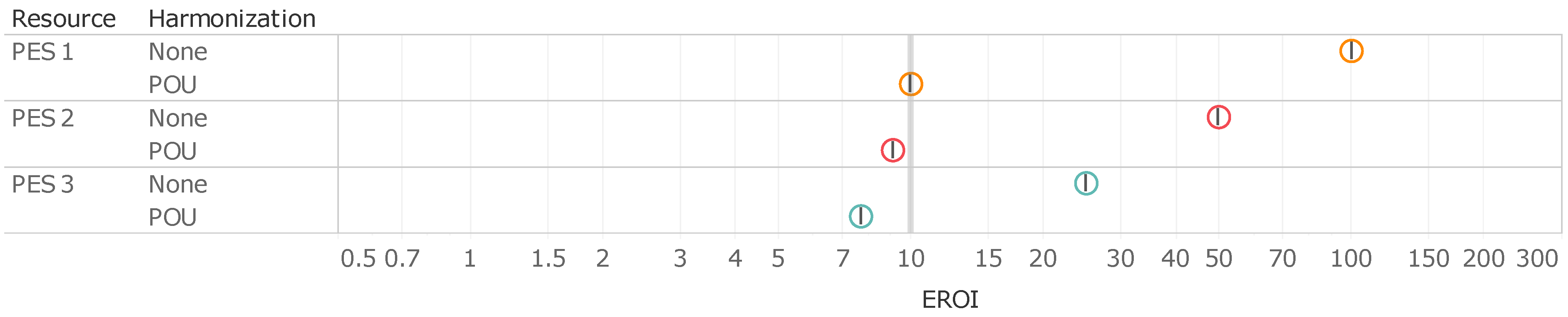
Figure 1. Streamlined energy systems diagram of the exploitation of a primary energy resource (PES) for the production of a useful energy carrier (EC). Inv1 = energy investment for resource extraction (E); Inv2 = energy investment for resource processing and delivery (P&D). S = energy sink (thermodynamic losses). Energy system diagram following the symbolic conventions introduced by Odum [18].
Sustainability 14 07098 g001
Figure 2. EROI “at point of extraction” vs. EROI “at point of use” for three fictional primary energy resources, highlighting the strong non-linearity in the relation between the two.
Sustainability 14 07098 g002
Figure 3. Net Energy Cliff diagram relating EROI and net energy expressed as proportion of the Gross Energy Output that is delivered to society. Arrows shows how the estimates of EROI and net energy change when extending from point-of-extraction to point-of-use.
Sustainability 14 07098 g003
Figure 4. Process chain for thermal fuels from extraction (1) to point-of-use (6).
Sustainability 14 07098 g004
Figure 5. EROI values for thermal fuels, respectively, as originally published (Harmonization = “None”) and post-harmonization at point of use (Harmonization = “POU”). CSG = coal seam gas; CTL = coal to liquids; LNG = liquified natural gas. Note use of logarithmic scale on horizontal axis, for a more meaningful representation of the significance of the relative differences in terms of net energy (cf. Section 2.4). * = gaseouas fuel; ο = liquid fuel; □ = solid fuel.
Sustainability 14 07098 g005
Figure 6. Harmonized EROI values for thermal fuels at point of use, plotted against their corresponding net-to-gross energy output ratios (“net energy cliff”). CSG = coal seam gas; CTL = coal to liquids; LNG = liquified natural gas. Note use of logarithmic scale on horizontal axis, for a more meaningful representation of the significance of the relative differences in terms of net energy (cf. Section 2.4).
Sustainability 14 07098 g006
Figure 7. EROI values for electricity, respectively, as originally published (Harmonization = “None”), and post-harmonization in terms of equivalent primary energy output, respectively assuming deployment in a thermal-dominated electricity grid mix (Harmonization = “PE eta = 0.3”), and deployment in a de-carbonized electricity grid mix (Harmonization = “PE eta = 0.7”). BECCS = bioenergy with carbon capture and sequestration; CSP = concentrating solar power; PV = photovoltaics. Note use of logarithmic scale on horizontal axis, for a more meaningful representation of the significance of the relative differences in terms of net energy (cf. Section 2.4).
Sustainability 14 07098 g007
Figure 8. Harmonized EROI values for electricity (assuming deployment in a thermal-dominated electricity grid mix, ηG = 0.3), plotted against their corresponding net-to-gross energy output ratios (“net energy cliff”). BECCS = bioenergy with carbon capture and sequestration; CSP = concentrating solar power; PV = photovoltaics. Note use of logarithmic scale on horizonal axis, for a more meaningful representation of the significance of the relative differences in terms of net energy (cf. Section 2.4).
Sustainability 14 07098 g008
Table 1. Calculation of EROI “at point of extraction” vs. EROI “at point of use” for three fictional primary energy resources, highlighting the strong non-linearity in the relation between the two.
Energy
Resource
Inv1PEEROI
“at Point of
Extraction”
= PE/Inv1
Inv2ECEROI
“at Point of Use”
= EC/(Inv1 + Inv2)
PES11100100910010
PES221005091009.1
PES341002591007.7
Table 2. For each stage (i) of the supply chain for each thermal fuel beyond extraction, the following values are reported: energy investment required at that stage (Invi), cumulative investment in the upstream chain up to that stage, excluding the investment for extraction ( 2 i I n v j ), and maximum EROI at that stage (EROIi,MAX), disregarding the investment for extraction (i.e., assuming infinite EROI at point of extraction). Data taken from Ecoinvent v3.7 and v3.8 [73]. All investments are expressed as % relative to the final energy “return” (i.e., the net available energy in the output fuel at point of use). A value of 0 means that that specific supply chain stage does not apply to that fuel.
Supply Chain Stage(2) Preparation(3) Transmission(4) Refining(5) Purification(6) Distribution
Fuel Inv2 2 2 I n v j EROI2,MAXInv3 2 3 I n v j EROI3,MAXInv4 2 4 I n v j EROI4,MAXInv5 2 5 I n v j EROI5,MAXInv6 2 6 I n v j EROI6,MAX
Oil001.5%1.5%678.9%10.4%9.6009.61.1%11.5%8.7
Gas007.7%7.7%1307.7%1307.7%1310.2%17.9%5.6
Coal4.2%4.2%245.6%9.8%1009.8%1009.8%1009.8%10
Bioethanol (Maize)000061%61%1.72.2%62.6%1.61.5%64.1%1.6
Bioethanol (Sugarcane)00002.5%2.5%392.2%4.7%2104.7%21
Bioethanol000033.6%33.6%3.02.2%35.8%2.8035.8%2.8
Biogas000.2%0.2%42000.2%42015.3%15.5%6.40.4%15.9%6.3
Biodiesel3.3%3.3%311.7%4.9%205.4%10.3%10010.3%10010.3%10
Wood Pellets51%51%2.0051%2.0051%2.0051%2.011.7%63%1.6
Table 3. Number of papers returned by the literature search, per resource type. The total number of papers in this table is more than that reported in Table 2 because some papers estimated EROI values for more than one technology or resource. BECCS = bioenergy with carbon capture and sequestration; CSG = coal seam gas; CTL = coal to liquids; LNG = liquefied natural gas.
Papers by Resource TypeInitial TallyPost-Screening Tally
Thermal fuels
Biofuels (including biodiesel, bioethanol, biogas)83
Coal (including CSG and CTL)92
Natural Gas (including shale gas and LNG)105
Oil (including Oil Sands)119
Electricity
BECCS32
Biogas40
Concentrated Solar Power21
Geothermal52
Hydropower72
Oceanic11
Nuclear Power31
Photovoltaics114
Wind Power105
Publisher’s Note: MDPI stays neutral with regard to jurisdictional claims in published maps and institutional affiliations.

