Article

Population, Wars, and the Grand Canal in Chinese History

1
Department of Geography and Resource Management, The Chinese University of Hong Kong, Shatin, Hong Kong, China
2
School of Geography, Nanjing Normal University, 1 Wenyuan Road, Nanjing 210097, China
*
Authors to whom correspondence should be addressed.
Sustainability 2022, 14(12), 7006; https://doi.org/10.3390/su14127006
Submission received: 21 April 2022 / Revised: 2 June 2022 / Accepted: 3 June 2022 / Published: 8 June 2022

Abstract

:
Throughout Chinese history, the Grand Canal served as a regional infrastructure in facilitating socio-economic and political development. The core regions of each dynasty were located in China’s eastern plain, and the Grand Canal ran from south to north through the plain, connecting northern and southern China. In unison, the areas along the Grand Canal also suffered from frequent wars. The role of the Grand Canal in influencing regional stability has yet to be sufficiently explored in the literature. This study seeks to (1) figure out the spatial distribution of population and wars, and (2) quantitatively measure the relationship between wars, population, and the distance from waterways in the Grand Canal Area in AD752–1910 by using their high-resolution geo-referenced data. Kernel density analysis was employed to serve the first purpose, while Pearson correlation and curve estimation analyses were applied to serve the second. Our results show that the areas surrounding the Grand Canal were densely populated. There was a war hot zone in the Beijing–Luoyang–Nanjing region near the Grand Canal, which shifted gradually over time. The correlation between war and population densities was positive, whereas the correlation between war density and distance from the waterway was negative. Finally, the cubic model captures the non-linear relationship between population, wars, and waterways. The above findings may shed more light on the Grand Canal’s role in influencing regional population and war patterns in historical China, a topic that has received little academic attention. More importantly, they may help advance empirical understanding of the impact of large-scale infrastructure on regional sustainability.

1. Introduction

The construction of the Grand Canal was completed in the Sui Dynasty (c. AD581–619), and it has long been a Chinese imperial symbol [1]. The Grand Canal was a functional regional infrastructure. It is notable for its caoyun transportation system (grain transportation and strategic logistics). The caoyun system made significant contributions to establishing a foundation for maintaining the centralization of authority and unity within the multinational country [2,3]. Each dynasty’s core region was located in China’s eastern plain, and the Grand Canal ran through the plain from south to north, connecting northern and southern China. The regions surrounding the Grand Canal were relatively prosperous and populated.
In the historical studies of the Grand Canal, Huang et al. [4] figure out that the rise and fall of Kaifeng mirrored the rise and fall of the Grand Canal from the Sui to the Qing Dynasties. Moreover, many ancient cities located near major waterways were primary hubs of rice cultivation for both armies and residences [5]. People traditionally lived near canals to secure water for agriculture and daily needs, making the canals more populated than the other areas [6]. On the other hand, the Grand Canal was frequently hit by wars. In the Tang Dynasty, An Lushan sparked the An–Shi Rebellion (AD755–763), undermining central authority and sparking both regionalism and separatism, while An Lushan’s forces damaged the Grand Canal’s accessibility [7].
Given the historical background, we can see that the areas along the Grand Canal were populated but suffered from frequent wars. Such a phenomenon was related to the “population-pressure-led social contradiction” [8], which might be attributable to the population growth along the Grand Canal. Nevertheless, the relationship between the population, wars, and the Grand Canal has not been investigated systematically. It is worth noting that there are various studies examining the geographical shifting [9], cultural influence [10,11], historical uniqueness [2,3], and infrastructure sustainability of the Grand Canal [12]. The special socio-ecological landscape created by the Grand Canal [13] and the making of the Grand Canal as a heritage site [14] are also highlighted. However, the main focus is still put on the role of the Grand Canal in facilitating regional development via increasing accessibility [4,15,16,17,18,19], at least in English literature. Briefly, there have been abundant research findings on the Grand Canal’s contribution to regional development and how the canal system differentiated the region from the others. On the other hand, the canal had a significant impact on the people who lived along with it. The Grand Canal had also changed the geographic pattern of the population significantly, forming some new densely-populated, yet conflict-prone, regions. As the role of the Grand Canal in influencing regional stability is insufficiently explored in the literature, we seek to address this research gap. There are two main objectives for us to fulfill in this study. First, we figure out the spatial distribution of population and wars. Second, we quantitatively measure the relationship between wars, population, and the distance from waterways.
It is worth noting that the most common research approach in sustainability studies is to make changes to existing facilities, monitor the changes, and compare the results to the initial conditions. One of the most prominent disadvantages of this approach is that people tend to conclude too quickly and on too small geographical scales [12]. Therefore, we base on the historical and geographic knowledge of the Grand Canal, which is one of the largest infrastructures in Chinese history, to examine the interconnection between population, wars, and waterways in the Grand Canal Area across different historical periods. Our research focus is on how the Grand Canal changed regional stability in the long term. We use war data combined with the corresponding spatial distribution of the population and the waterways to analyze their interrelationship. Using past experiences as a guide, our findings may contribute to a better understanding of the impact of large-scale infrastructures on regional sustainability.

2. Scope of Research and Data

2.1. Study Period and Study Area

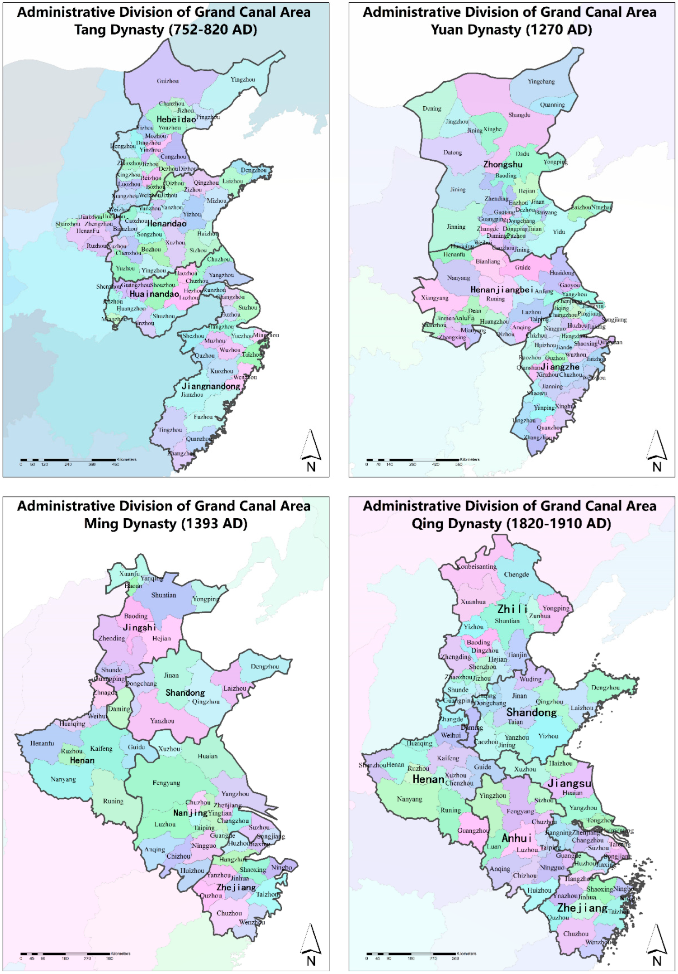
Our data include the population, wars, and waterway systems in the Grand Canal Area. Considering the availability of the fine-grained population data, the periods of AD752–820, AD1270–1393, and AD1820–1910, which included the four Chinese dynasties, namely, Tang (c. AD618–907), Yuan (c. AD1271–1368), Ming (c. AD1368–1644), and Qing (c. AD1636–1912), are examined. The starting years of the three periods are the years of prosperity and stability of the dynasty, characterized by population growth and fewer wars. The end years of the chosen periods are marked by social recovery and resilience. In between, there are times of social unrest and frequent wars.
The Grand Canal Area is relatively large. The canal flows through the provinces and cities in the east of China, such as Beijing, Tianjin, Hebei, Shandong, Henan, Anhui, Jiangsu, and Zhejiang. Nevertheless, the administrative boundaries of the Grand Canal Area and its sub-regions varied in different dynasties. Considering the scope of this study, we take the first-level administrative regions covering the Sui–Tang Canal and the Beijing–Hangzhou Canal of the corresponding dynasties as the Grand Canal Area. Moreover, the area’s second-level administrative areas are also vectored to match the spatial resolution of the population data. The geographic coverage of the administrative areas refers to the administrative divisions of the corresponding dynasties according to the Chinese Historical Atlas [20] and the Chinese Civilization in Time and Space [21]. Table 1 lists the first-level administrative divisions of the various dynasties concerned, while Figure 1 shows the administrative areas of the Grand Canal Area in different periods. The first-level administrative areas of the Grand Canal Area include mainly the North China Plain, Huanghuai Plain, and the middle and lower reaches of the Yangtze River. The basic form of the canal area is relatively constant, which is crucial for us to extract and process war and population data over different periods.

2.2. Population Data

We obtain our population data from the Chinese Population History [22], covering the six time-sections, namely AD752, 820, 1270, 1393, 1820, and 1910. Population data for the Tang Dynasty cover the 11th year of Tianbao (AD752) and the 15th year of Yuanhe (AD820). The original AD752 population records come from the geographical section of the Old Book of Tang. In contrast, the original AD820 population records come from the Yuanhe Maps and Records of Prefectures and Counties. Temporally, the population size ratio between AD752 and AD820 is used to interpolate the missing values. Spatially, the missing data are interpolated by averaging the values of the neighboring cells.
The population data of the Yuan Dynasty cover the beginning of the Yuan Dynasty (AD1270). The original data come from the geographical book of the History of Yuan. The population estimation and adjustment methods are the same as the Tang Dynasty. Population data for the Ming Dynasty cover the 23rd year of Hongwu (AD1393). The population size in the early Ming Dynasty was precisely recorded in the History of Ming due to the population registration system. Despite changes in the administrative divisions during the period, there were few changes in the second-level administrative areas. Therefore, we re-organize the population data based on the second-level administrative areas and map the population through the administrative divisions of the late Ming Dynasty.
Population data of the Qing Dynasty cover the 25th year of Jiaqing (AD1820) and the 2nd year of Xuantong (AD1910). The original AD1820 population records come from the Jiaqing Yitongzhi. The original AD1910 population records come from the household registration survey conducted by the Ministry of the Interior in the late Qing period. There were no major changes in the administrative divisions in the Grand Canal Area during the Qing Dynasty, and the population records are relatively complete. As the accuracy of the data is higher than in other historical periods, data correction and interpolation are not required.

2.3. War Data

Our war records are obtained from the Chinese Military History [23]. The records cover the period from 800BC to AD1911, with information such as the year the war began, the participants, the locations, and its causes included. Wars are counted based on the number of battles. The spatial locations of the wars are geo-referenced according to the current county-level administrative boundaries in China. The war data are converted to vector data. The attributes of the war data include the outbreak years of the wars and their geographical locations at the county level.

2.4. Data Aggregation

Based on the time sections of the population data, the population and the war data are aggregated in three periods. The first period is AD752–820, extending from the Tang to the late Tang Dynasties, including the An–Shi Rebellion that affected the entire country. The second period is AD1270–1393, spanned between the heyday of the Yuan Dynasty and the stable period of the early Ming Dynasty. This period covers the wars during the transition from the Yuan to the Ming Dynasties. The third period is AD1820–1910, from the time before the outbreak of the Opium War to the establishment of the Republic of China, covering the Taipei Rebellion. The timespan of each period is approximately 100 years and includes major war disturbances. Such consistency facilitates the comparison between different periods.

3. Methods

This research consists of two parts. The first part is to figure out the spatial distribution of population and wars. It is more accurate to use population density and war density in figuring out their patterns. The distribution patterns in different periods are then compared to trace their spatio-temporal evolution. The second part is to quantitatively measure the relationship between wars, population, and the distance from waterways. We calculate the Pearson correlation coefficients between wars, population, and the distance from waterways. The result is further verified by the curve estimation method to reveal the possible non-linear effect of the population density and the distance from waterways on wars.

3.1. Population

The population density is calculated based on the population data of the second-level administrative areas and the area of the corresponding administrative divisions. The unit is the number of people per square kilometer. The calculation method is as follows:
D = P A  
where D represents the number of people per km2, P is the total number of people in the secondary administrative region, and A is the area of the secondary administrative region in km2.
When classifying population density, we need to consider the difference between the total population in different periods and the expression of the difference in population density [24]. The number of grades and the range of each level should fully reflect the population density characteristics. Regarding the number of grades, the population density of the Tang Dynasty is fewer than that of other periods due to the relatively smaller population size during the time. Therefore, the population density in the Tang Dynasty is divided into seven grades, and that in the other periods is divided into nine grades. In the three time-sections in the Tang and Yuan Dynasties, 5, 10, and 20 are used to indicate the differences in population level. In the three time-sections of the Ming and Qing dynasties, 5, 10, 20, and 100 are used to indicate the differences in population level. Figure 2 shows the final population density in different periods.

3.2. War Distribution and War Belt Identification

The war data are at the county level, and their digitization is made according to the online maps provided by the Tiandi Map. According to the center points of the main urban areas corresponding to the county-level units, we obtain the geographic coordinates and add them with the outbreak years of the wars to the attribute tables [25]. The vectored contents are AD752–820, 1270–1393, and 1820–1910. There are 1679 war records, with 577 war points in AD752–820, 498 war points in AD1270–1393, and 604 war points in AD1820–1910. The principal wars of the three periods are the An–Shi Rebellion in AD752–820, the rebellion in AD1270–1393, and the Taiping Rebellion in AD1820–1910. When fitting the population–war–river relationship, war points in the Grand Canal Area are selected for further analysis. Since the wars during the transition between the Yuan and the Ming Dynasties involved two different administrative divisions, their overlapped parts in the two dynasties are chosen for the analysis.
Since the war data are in the point layer, population density is in the surface layer corresponding to each secondary administrative area, and the waterway data are in the line layer, we need to standardize the data format before exploring their relationship. The spatial distribution of wars is expressed by the density of war spots. We calculate the point density by using the Kernel Density Function, assuming that a smooth curved surface covers each point and that the surface value is the highest at the location of the point. The surface value gradually decreases when the distance from the point increases, and the distance from the point equals the search radius. The surface value at the search radius boundary is zero. Only circular neighborhoods are allowed. The volume of the space enclosed by the curved surface and the plane below is equal to the value of the weight field assigned to this point. When we specify the value of this field as none, the volume is one. The density of each output raster cell is the sum of the values of all the core surfaces superimposed at the center of the raster cell. The kernel function is based on the Quadratic Kernel Function [26] shown as follows:
f h ^ ( x ) = 1 / n i = 1 n K h ( x x i )
where K stands for the kernel, which is a non-negative function, the value after integration is 1, and h is the smoothing parameter, also called bandwidth, which is the search radius mentioned above.
The calculation of the kernel density is based on the war points in the three periods, and the resulting raster layer is expressed by the number of floating points. The value is determined by the raster calculation as an integer for subsequent data extraction. The war density range of the three periods obtained is 0–1080 in AD752–820, 0–785 in AD1270–1393, and 0–819 in AD1820–1910. From the numerical values of the war density and the number of war spots, the highest war density dropped from the Tang to the Qing Dynasties, indicating that the war distribution became more extensive. Finally, the aggregation of the Grand Canal regional wars is made within the current administrative divisions. The integration of the war density in the Grand Canal and the waterways’ locations is shown in Figure 3.
The above analysis is based on the overall war density. To further express the spatial distribution of the wars and eliminate data noise, the study extracts the hot zone of wars that passes through the center point of the war hot zone. The definition of the war hot zone is unified. The classification of the level of war density is expressed as quantiles, each of which contains an equal number of elements. It is assumed that the change in the density of the war points is linearly distributed, and the war points are divided into ten levels. The quantile assigns the same number of data values to each class and finally extracts the points of the first two classification sets (i.e., extracts the top 20 percent of the data points). There are no empty classes in the quantile classification, and there are no classes with too many or too little data. According to the results of quantile extraction and the basic situation of historical urban development along the Grand Canal [27], high-value bands of war distribution are extracted (Figure 4).

3.3. Statistical Analysis

The spatial relationship between the waterways and population is measured by extracting the spatial pattern of wars, which considers war density the dependent variable. In contrast, population density and distance from the waterway are the explanatory variables. As mentioned above, wars are expressed in the point layers, and the calculation of the kernel density of wars is associated with other surrounding war points. In contrast, the secondary rivers (waterways) in the Grand Canal Area are expressed in the line layers. The population density in the secondary administrative area is presented as the surface layers. As two time-sections are involved, the difference in population density between the two time-sections is used to represent the changes in population density. Therefore, when integrating data, each war point is used to extract changes in population density at its location. The distance from each war point to the nearest secondary river is calculated. Finally, the attributes of population density and the war–river distance are combined with the war density for subsequent correlation and regression analyzes.
We calculate the correlation between the three variables (i.e., war, population, and distance from the waterway). All of the skewness and kurtosis statistic values are less than ±1, indicating that our data are normally distributed (see Appendix A). Hence, Pearson correlation is applied [28] (Table 2). To reveal the possible non-linear effect of the population density and the distance from waterways on wars, we employ ten different curve-fitting models to generate their results. A separate model is generated for each dependent variable. Those models include Linear, Logarithmic, Inverse, Quadratic, Cubic, Compound, Power, S-curve, Growth, and Exponential. The details of those models can be found at https://www.ibm.com/docs/en/spss-statistics/28.0.0?topic=estimation-curve-models (accessed on 20 April 2022). The Logistic model is excluded in this study because our data are interval data. In evaluating different models, their R2-values and F-values are compared. The sum of squares, Akaike information criterion (AIC), and Bayesian information criterion (BIC) values of those models are also provided for reference (Table 3 and Table 4). The curve estimation in different periods is also presented in the tables.

4. Results

4.1. Population Distribution

Figure 2 presents the population density maps in six time-sections. The spatial patterns of the population density in the Grand Canal Area and their evolution in history are revealed. First, the area’s total population constantly increased, but with periodic fluctuations, so did the population density. Second, the following characteristics from the changes in population density in the Grand Canal Area can be found:
Hangzhou and Nanjing were densely populated consistently, and their population density increased continuously to be the most densely populated parts within the Grand Canal Area. Hangzhou was a crucial waterway station and experienced remarkable growth in the Sui Dynasty. Since the Tang Dynasty, the city as the capital had grown into an affluent metropolis with many merchants and inhabitants [29]. Similarly, Nanjing was a textile and minting industry hub beginning with the Sui and Tang regime, thanks to its advantageous geographical position and convenient transportation links. It became the capital of the Ming and Yuan Dynasties and remained prosperous and densely populated [30]. Those cities designated as the capital cities often had high population density.
On the other hand, the population density in the northern part of the Grand Canal Area fluctuated. Before the Tang Dynasty, more than three-quarters of the total population lived in the north, located between Qinling and Huaihe River, due to agricultural development and military factors having adequate troops to defend against northern nomads [31]. However, especially in the mid-8th century, when the An–Shi Rebellion occured, a mass peasant migration from the north to the south (such as Jiangxi and Fujian) to evade the rebellion occurred [32], resulting in a rapid population decline in AD752–820. Then, the population increased continuously until AD1910, reaching a level roughly equivalent to that of the southern part of the Grand Canal Area. The availability and improvement in rice production and innovative technology of maize adoption were the main reasons for Qing population growth [33].
There were densely populated areas along the canals, but they changed with the locational shifts of the canals. Figure 2 shows that the areas along the Sui–Tang Canal were densely populated in the Tang Dynasty. However, since the Yuan government modified the canal and built the Beijing–Hangzhou Canal [34], the densely populated areas gradually shifted eastward and were located along the Beijing–Hangzhou Canal. This phenomenon was more evident in the late Qing Dynasty, and a pronounced densely-populated zone was situated along the Beijing–Hangzhou Canal in AD1820–1910.
The population density on the coastal side of the Grand Canal Area steadily increased since there were comprehensive waterway networks and directly brought agricultural-economic development around the coastal Grand Canal. In the Tang Dynasty, the population density in the coastal area was the lowest in the Grand Canal Area. This can be seen from Figure 2 that the change in population density was affected by the shifting of the canals and by wars. For instance, in the Tang Dynasty, the reduction in population density mainly occurred in the northern part of the Grand Canal Area, where An Lushan cut off the waterway access to destroy the economic link between the north and south [7]. Liu Zhan, a Tang loyalist, contemplated rebellion with the army by blocking the northern Grand Canal and Luoyang. As canals could provide water resources and internal military communication, they were destruction targets for insurgents to disrupt the emperor’s food supply foundation and economic and political strengths. Thus, the attack caused casualties and massive migration from areas surrounding the Grand Canal to the south [35].
In the Ming Dynasty, the population density in the Grand Canal Area was roughly the same as the inland population. Influenced by natural calamities such as superstorms and famine after severe floods, the Mongolian provinces of Huguang and Jiangxi had more than half of the total grain revenue, and the Yangtze Delta was hard to function, resulting in scarce rice production [36]. Neither inhabitants living in the coastal areas nor inland areas could escape from the disasters, which caused the food shortage and residence destruction. In the late Qing period, the population density in the coastal area increased rapidly and became a very densely populated zone. Under the Treaty of Nanking Remer and the commercial port opening of Shanghai, the export of silk and nankeens from Nanjing had a substantial development. The prosperous enhancement fostered population amounts in southeast coastal areas with better employment opportunities and living quality [37].

4.2. War Distribution

Figure 3 shows the war kernel density in the Grand Canal Area. In the first three parts of the figure, the war density exhibited spatial clusters in three different historical periods. Still, the clusters in different historical periods had different characteristics. The fourth part of the figure calculates and expresses the density distribution map of all war points in the current administrative divisions. Briefly, during the Tang Dynasty, the areas of highest war density were mainly located in the northern part of the Grand Canal, the middle and lower reaches of the Yellow River, and the Fenhe River Basin. Tracing its history back to the late Sui Dynasty ruled by the Empress Wu Zetian, regions in northern China were subject to the frequent invasions by the Tibetan, Turk, and Khitan, causing Emperor Tang Xuanzong to set up ten military towns in the northern part of the Grand Canal Area so that the dominion could be safeguarded from northeast and northwest minority invasions. Nevertheless, province separatism in the north gave rise to An Lushan mutiny in AD755–763 controlling the northern Grand Canal to further attack the capital Changan in the Yellow River Basin [7]. Hence, the capital was assaulted by provincial armies nearly 100 times in the late Tang period [38].
On the other hand, wars in the Yuan and Ming Dynasties were concentrated in the southern part of the Grand Canal Area, particularly in southern Anhui and southern Jiangsu. More than 80% of Yuan inhabitants lived in the south of the Yangtze River Delta, which was the fundamental grain production and wealth accumulation transferred to the north government through the Grand Canal [36]. Therefore, there would be waging wars for attackers to cease the grain source and military support. Red Turbans, led by Zhu Yuanzhang, conquered the Yangtze Delta in AD1352–1368 [39]. In both Yuan and Ming Dynasties, dense distribution of masonry walls was constructed in the Yangtze River Delta [40], especially in Anhui, Jiangsu, and Zhejiang [41]. This can reflect that those places with flat terrain located at the southern Grand Canal were vulnerable and prone to wars.
In AD752–820, in the northern areas of the Sui–Tang Canal and the Beijing–Hangzhou Canal, an apparent war hot zone was located along the canals. In contrast, the war density in the southern part of the Grand Canal only concentrated in a small area. However, the war hot zone in the south gradually expanded in AD1270–1393 and AD1820–1910. The distribution of war had a strong connection with the geographic location of the waterways. The waterways provided water resources for troop communication and weapon transmission. This acted as a confronting strategy to raise resistance [42]. Figure 3 shows that both the southern and northern parts of the Grand Canal had more war spots distributed evenly along the waterways linked to the canals.

4.3. War Belt

Figure 4 shows that the war belts in the Grand Canal Area in different periods were similar but had different characteristics in specific locations. The center of the war belt was the Luoyang area, which extended north–south. The first three parts of Figure 4 show that in the Tang Dynasty, the center of the war belt was the Luoyang-Xi’an area, extending from Luoyang along the Sui–Tang Canal, and Xi’an was the starting point of the war belts along the Fen River in the north. Attackers invaded along the Grand Canal to reach the dynasty’s capital and usurp the throne.
In the Yuan and Ming Dynasties, the war belt stretched along the Luoyang canal. The basic form of the war belt in the Qing Dynasty remained roughly the same as in the previous periods, but the northern end centered around Luoyang shifted eastward from the Sui–Tang Canal to the Beijing–Hangzhou Canal. One of the intentions of building canals was to ship agricultural products and economic goods to the northern emperor to sustain northern China. This also encouraged people to settle down around the south-eastern of the canal, where cultivated lands, water resources, and employment opportunities were relatively abundant. However, when the dynasty declined, there might be risks of rebellion among impoverished people. The greater the number of people, the higher the opportunities to recruit an adequate group for rebellion [43]. A financially self-sustained area with tools and food suppliers was beneficial to long-term mutiny [44]. More importantly, a populous area with a huge tax base reflecting the most valuable places monitored by the ruler was usually targeted to be a war location since this could let the emperor suffer the psychological and reputational consequences of demonstrating to a vast population that the emperor was unable to safeguard their homeland [44]. Therefore, the wars were largely concentrated along the canals with recruitment base, resources supply, and vulnerable population.
The wars were distributed in the Huanghuai Plain to form a branch line. Figure 4 shows that the war belts are mainly concentrated in the Jiangnan and North China regions. The Huanghuai Plain connecting these two areas had a low war density. The main reason is that the area is situated in the flood zone of the Yellow River and the Huaihe River. Between the late Ming and Qing, dyke breaching and rising riverbeds were frequent, almost three times a year [45,46]. This inundated the entire Huanghuai Plain, causing crop failure and heavy population casualties [47]. In addition, extreme weather, especially floods, brought significant changes in the regional population. This lack of large cities led to a low military-strategic value there. Therefore, hazard-prone regions like Shandong have less possible recruitment of rebellion and were less likely to be a war target.
The war distribution is strongly correlated with the geographic distribution of canals and waterways. After combining the war points in the three periods between AD752–1910 to calculate the war kernel density, we find the high-density war areas. The white line in the fourth part of Figure 4 shows that wars distribution is concentrated in Luoyang along the canal, while in the southern area, a branch line along the Yangtze River is formed, with Nanjing as the center. A branch line along the Fen River is formed in the northern area, with Xi’an as the center. These three cities are considered the ‘Great Ancient Capitals’ that symbolize the Chinese dynasties in different periods. Focus on our study period, Tang (AD618–907) had its capital at Xi’an, being formerly the Silk Road’s starting point. At the beginning Ming Dynasty (AD1368–1644), Nanjing was chosen as the capital where traditional farming flourished thanks to the pleasant environment and a strong economy. The eastern capital of Tang was Luoyang in the Central Plain, which was the birthplace of imperial Chinese agricultural civilization [48]. They commonly incorporate political systems and economic hubs linking the Grand Canal to the south. Capitals were undoubtedly the foci of wars due to their center of the regime and political power. Rebellious movement usually involved conquering and occupying the capitals by destroying the ruler’s army across waterways to control water resources and cease the transportation lines from the south to the emperor’s hand.
The war belts reflect the characteristics of the wars’ geographic distribution. The war distribution in the Grand Canal Area was closely linked to the geographical location of the canal. Combining the spatial characteristics of the three periods of war can provide a basic understanding of this. Concrete examples include that the An–Shi rebellion in the Tang Dynasty erupted from Beijing and spread to Luoyang and Xi’an, forming a war hot zone in the north. The rebellion in the late Yuan Dynasty began in the central and southern Anhui before it spread northward, forming the southern war hot zone. Similarly, the Qing Dynasty Taiping Rebellion erupted from Guangxi and extended to the north, eventually forming a war center in the Jiangnan region [49].

4.4. Statistical Relationship among Population Change, War Density, and Distance from the Waterway

After figuring out the geographical distribution of population and wars in the Grand Canal Area, we further examine the interrelationship between population change, war density, and distance from the waterway via statistical analysis. Regarding the correlation results (Table 2), the correlation between population change and war density was the highest. The two variables were positively correlated, indicating that the war density was relatively higher in areas with drastic population growth. On the contrary, the correlation between war density and distance from the waterway was weaker and in negative value. The correlation between population change and distance from the waterway was the weakest and in negative value.
Regarding the temporal comparison, whether in the nationwide and the Grand Canal Area, the relationship between population change and war density slightly declined from the Tang to the Ming Dynasties. However, in the Qing Dynasty, the relationship bounced back and reached a new height. In parallel, the correlation between the war density and the distance from the waterway gradually increased. The Grand Canal Area and the nationwide findings were similar, implying that the Grand Canal Area could epitomize the general situation of the whole of China.
We explore the possible non-linear relation between population change, war density, and distance from the waterway. Table 3 and Table 4 show that the curve fitting results are quite different. Regarding the relationship between population change and war density, the cubic models give the biggest R2. The corresponding F-values are relatively smaller (Table 3), indicating that it is most appropriate to use the cubic model to capture their relationship. However, the fitting results between war density and distance from the waterway are not as good as between war density and population change. Still, the cubic model gives the biggest R2 (Table 4). Therefore, we choose the cubic model to model war density with population change and distance from the waterway.
Here, we use war density as a dependent variable and population change and distance from the waterway as independent variables. The model is presented below:
y = b 1 + b 2     P + b 3     P 2 + b 4     P 3 + a 1 + a 2     R + a 3     R 2 + a 4     R 3
In the model, y is the war density at the specific location, P is population change, and R is the distance from the waterway. a and b are the parameters, and their initial values are 1. The model is iterated based on the initial parameters. When the residual sum of the parameters and the estimated value of the model stabilize or reach the convergence standard, the model will cease to iterate [50]. The final iteration result and the parameters for each period are listed in Table 5. The table shows that the differences between the models in different historical periods are obvious, and the values of R2 are different in the three periods. The model and the parameters in the three periods are stated below:
AD752–820
y = 15.201 P 0.154     P 2 + 0.001     P 3 + 3.601 R 0.07     R 2 + 151.1
AD1270–1393
y = 1.917 P + 0.003     P 2 1.38 R + 0.023     R 2 + 415.5
AD1820–1910
y = 1.123 P 1.383 R + 0.006     R 2 + 384
The above models show a strong non-linear relationship between population change and war density in the Tang Dynasty. However, this relationship became linear in the Qing Dynasty, indicating that their relationship had changed. Furthermore, the relationship between the distance from the waterway and war density gradually changed from non-linear to linear from the Tang Dynasty to the Qing Dynasty.

5. Discussion

This study uses the population and war data together with the location of the waterways in the Grand Canal Area to explore their spatio-temporal dynamics. We find that the densely populated areas concentrated along the canal channels while they were subsequently affected by the shifting of the canals. In the Tang and the Yuan Dynasties, there were two population clusters located along the Sui and Tang Canals, and the branch line occurred in the eastern and southern regions of Shandong. After the Ming Dynasty, the population of this area increased continuously, forming an apparent belt running through the north and south and spreading along the canal (Figure 3). This phenomenon might be due to a significant increase in the regional population brought by migration from the early Ming Dynasty, which moved the population of Shanxi to the Huanghuai Plain to support economic recovery during the time [51]. Moreover, the development of trans-shipment canal trade along the shipping cities boosted the socio-economic development along with the canal areas. Canal cities and populations continued to grow on this basis, making the population concentrated along with the distribution of the waterways [52].
On the other hand, the Grand Canal Area had more frequent wars in our study periods. This phenomenon was manifested in Luoyang, as the center stretches from the north to the south to form a war hot zone along the canal. This war zone exhibited different characteristics in different periods. The war hot zone was branched along the Fen River in the Tang Dynasty, while the war hot zone was branched along the Yangtze River after the Yuan Dynasty. With the change of the canal, the war hot zone gradually shifted eastward. Although the spatial distribution of high-density war areas had a historical contingency, it was also constrained by the physical environment and social development [53]. This is evident in the Grand Canal Area, where most of the Tang Dynasty wars were distributed in the northern part of the canal, which was closely linked to the geographical distribution of population and economic centers at that time. With the gradual shift of China’s economic center to the south, the war hot zones also moved south, forming stable high-density war areas in the lower reaches of the Yangtze River [54]. It can be seen from the overlay of war belts of different periods in Figure 4 that war belts in the northern part of the Grand Canal were located along the canal. In contrast, in the southern region, due to more complicated waterway systems, the spatial distribution of war points is a bit different. The specific manifestation is that a branch line along the Yangtze River was formed after the Yuan Dynasty.
The war density in the Grand Canal Area was positively correlated with the change in population density. Every citizen has an equal and continual opportunity to participate in a rebellion [43]. The concept of ‘conflict proclivity per capita’ states that the higher the population, the greater the risk of wars [55]. Populations were the source of war resources since there would possibly be a strong recruitment group when there was a large population. This group might also tend to destroy populated areas to minimize the agricultural and economic bases.
On the other hand, the war density was negatively correlated with the distance from the waterway. Those states with finite reach might find it difficult to regulate activity outside their existing infrastructure [56]. Locations far from the capital, on the other hand, may be prone to conflict because the population’s preferences were likely to diverge significantly from those of the emperor and because it was hard for the government to manage remote territory [57]. Even if the government created military bases around the region to mitigate the effects of distance, these bases were backed by shaky supply lines and became targets for rebel groups [58]. This may explain why the Grand Canal Area was conflict-prone.
Our statistical results show that the correlation coefficient between war density and population density in the Grand Canal Area was ~0.5, while the one across China was ~0.3, indicating that the population-war relationship in the Grand Canal Area was stronger. Whether nationwide or in the Grand Canal Area, the correlation coefficient of war density and river distance was approximately −0.3. The population–war correlation increased over the three periods, while the river–war relationship remained relatively constant. This shows that wars in the Grand Canal Area were more closely linked to the population, higher than average. This echoes the previous studies about wars in Chinese history, which were mainly brought by population pressure rather than by the environmental and climatic variables [59,60]. This study further extends it to regional infrastructure. In addition, the effects of population density and war–river distance on war density are curvilinear. This indicates that the inter-relationship between population, wars, and the canal was interactive. Moreover, it might be about the threshold concept, while the human–environment relationship became strongly significant once the threshold had been reached [61]. Further investigation should be made along with this rubric.
From the perspective of military geography, the North–South regime confrontation in terms of the united empires south of the Great Wall versus nomadic tribes/polities in the steppes of Inner Asia drove the secular war–peace cycles of Chinese history [62,63,64]. Specifically, China had nine strategic areas, including four corners (Guanzhong, Hebei, Southeast China, and Sichuan), four foci (Shanxi, Shandong, Hubei, and Hanzhong), and the heartland (the Central Plain) [65]. Furthermore, war hotspots were located in the Loess Plateau and the North China Plain during warm and wet periods, but in the Central Plain, Jianghuai region, and lower reaches of the Yangtze River Delta during cold and dry periods [8,66]. Compared to previous studies, we narrow the scope of the analysis from the national to the regional levels. Our study area is overlapped with the Central Plain, the Jianghuai region, and the lower reaches of the Yangtze River Delta. That region was quantitatively identified as a war hotspot in recent studies [8,66]. Here we supplement that the war hot spot was located precisely along the Grand Canal (i.e., the Beijing–Luoyang–Nanjing region), which is attributable to the population growth in the Grand Canal Area. This finding may help provide a more nuanced picture of the military geography of historical China.
As our research findings also reveal the apparent importance of space and geographic locations, the application of spatial econometrics [67] and spatial analysis [8,66] in examining the nexus between population, wars, and the canal can be explored.

6. Conclusions

Grand Canal is one of the largest infrastructures in Chinese history. This study investigates the geographic distribution of population and wars in the Grand Canal Area and explores their long-term spatio-temporal dynamics. There was spatial clustering of population and wars in the Grand Canal Area in different historical periods. Moreover, population change and distance from the waterway were negatively correlated, while population change and war density were positively correlated. Furthermore, the distance from the waterway had a negative effect on war density. The cubic model successfully captured the effect of population change and distance from the waterway on war density. Briefly, the densely populated areas of the Grand Canal Area were more prone to wars. The above findings may shed more light on the Grand Canal’s role in influencing regional population distribution and social stability in Chinese history, a topic that has received little attention in academia. More importantly, they may help advance empirical understanding of the impact of large-scale infrastructures on regional sustainability. On the one hand, large-scale infrastructures could promote regional development and population growth. On the other hand, they could raise the likelihood of violent conflicts. Perhaps the role of large-scale infrastructures in affecting human societies should be further investigated.

Supplementary Materials

The following supporting information can be downloaded at: https://www.mdpi.com/article/10.3390/su14127006/s1, The bigger version of the individual figures in Figures S1–S4.

Author Contributions

Conceptualization, H.F.L. and B.J.; methodology, H.F.L. and B.J.; formal analysis, H.F.L., X.J. and B.J.; investigation, H.F.L., X.J. and B.J.; resources, H.F.L., X.J. and B.J.; data curation, H.F.L., X.J. and B.J.; writing—original draft preparation, H.F.L., X.J. and B.J.; writing—review and editing, H.F.L., X.J. and B.J.; visualization, B.J.; supervision, H.F.L.; project administration, H.F.L.; funding acquisition, H.F.L. All authors have read and agreed to the published version of the manuscript.

Funding

This research was funded by the Improvement on Competitiveness in Hiring New Faculties Funding Scheme (4930900) of the Chinese University of Hong Kong.

Institutional Review Board Statement

Not applicable.

Informed Consent Statement

Not applicable.

Data Availability Statement

The datasets analyzed during the current study are available from the corresponding author on reasonable request.

Acknowledgments

We thank Teodora Morar for her valuable comments on the manuscript.

Conflicts of Interest

The authors declare no conflict of interest.

Appendix A

Table A1. Normality test results for the variables employed in this study.
NMeanUnitSkewnessKurtosis
StatisticsStd. ErrorStatisticsStd. Error
Population density472117.84person/km20.469 0.412 0.432 0.524
War density393832.84km (distance between war points)0.465 0.580 0.210 0.260
Distance from waterway155936,861 m0.252 0.303 0.383 0.406

References

  1. Ye, S. The Grand Canal in Republican China. J. Econ. Soc. Hist. Orient 2019, 62, 731–772. [Google Scholar] [CrossRef]
  2. Rong, Q.; Wang, J. Interpreting heritage canals from the perspective of historical events: A case study of the Hangzhou section of the Grand Canal, China. J. Asian Archit. Build. Eng. 2021, 20, 260–271. [Google Scholar] [CrossRef]
  3. Zhang, M.; Lenzer, J.H., Jr. Mismatched canal conservation and the authorized heritage discourse in urban China: A case of the Hangzhou Section of the Grand Canal. Int. J. Herit. Stud. 2020, 26, 105–119. [Google Scholar] [CrossRef]
  4. Huang, W.; Xi, M.; Lu, S.; Taghizadeh-Hesary, F. Rise and fall of the Grand Canal in the ancient Kaifeng City of China: Role of the Grand Canal and water supply in urban and regional development. Water 2021, 13, 1932. [Google Scholar] [CrossRef]
  5. Boelens, L.; Dong, W.; Wang, Y. The interaction of city and water in the Yangtze River Delta, a natural/artificial comparison with Euro Delta. Sustainability 2018, 10, 109. [Google Scholar]
  6. McCool, S.F.; Clark, R.N.; Stankey, G.H. Water and People: Challenges at the Interface of Symbolic and Utilitarian Values (Gen. Tech. Rep. PNW-GTR-729); U.S. Department of Agriculture, Forest Service, Pacific Northwest Research Station: Portland, OR, USA, 2008. [Google Scholar]
  7. Jennifer, W.J. An Lushan (An Shi) Rebellion. In Berkshire Encyclopedia of China: Modern and Historic Views of the World’s Newest and Oldest Global Power; Cheng, L., Ed.; Berkshire Pub. Group: Great Barrington, MA, USA, 2009; pp. 49–52. [Google Scholar]
  8. Zhang, S.; Zhang, D.D.; Li, J. Climate change and the pattern of the hot spots of war in ancient China. Atmosphere 2020, 11, 378. [Google Scholar] [CrossRef] [Green Version]
  9. Wang, X.; He, H.; Zhou, Y.; Gao, C.; Han, S. Analysis of remote sensing archaeology on traffic function transformation of Tongji Grand Canal in Sui and Tang Dynasties. Chin. Geogr. Sci. 2006, 16, 95–101. [Google Scholar] [CrossRef]
  10. Wang, F.; Li, H.; Liu, Q.; Du, L. Bottom-up or top-down? The Water God faith in human-water relationships: A case study of the Beijing-Hangzhou Grand Canal in the Qing Dynasty. In Water-Related Urbanization and Locality; Wang, F., Prominski, M., Eds.; Springer: Singapore, 2020. [Google Scholar]
  11. Qu, B.; Tang, S.; Zeng, J. A study of the Grand Canal culture from stories from a Ming collection. In Proceedings of the 2020 2nd International Conference on Education, Economics and Information Management (EEIM 2020), Shanghai, China, 19–20 December 2020. [Google Scholar]
  12. Tsung, N.; Corotis, R.; Chinowsky, P.; Amadei, B. A retrospective approach to assessing the sustainability of the Grand Canal of China. Struct. Infrastruct. Eng. 2013, 9, 297–316. [Google Scholar] [CrossRef]
  13. Xu, L.; Peng, X.; Jiang, H.; An, X.; Xi, X. Distributive hydraulic engineering, cross-scale landscape planning, and climate change resilience: On the water-adaptive strategy in the Huai’an–Yangzhou Section of China’s Grand Canal. River Res. Appl. 2022. [Google Scholar] [CrossRef]
  14. Yan, H. The making of the Grand Canal in China: Beyond knowledge and power. Int. J. Herit. Stud. 2021, 27, 584–600. [Google Scholar] [CrossRef]
  15. Cheung, S.W. Construction of the Grand Canal and improvement in transportation in late imperial China. Asian Soc. Sci. 2008, 4, 11–22. [Google Scholar] [CrossRef]
  16. Wang, F.; Gao, C.; Hu, W. The influence of water transportation evolution on the economic development of cities along the Beijing–Hangzhou Grand Canal since the Late Qing Dynasty. In Water-Related Urbanization and Locality; Wang, F., Prominski, M., Eds.; Springer: Singapore, 2020; pp. 27–45. [Google Scholar]
  17. Li, S.; Guo, W. The functions of the Jing-Hang Grand Canal and the development and utilization of its North Jiangsu section. Quat. Sci. 2007, 27, 861–869. [Google Scholar]
  18. Wang, L. The Grand Canal and the rise and development of urban civilization of Zhenjiang. J. Nantong Univ. (Soc. Sci. Ed.) 2008, 24, 21–24. [Google Scholar]
  19. Liu, Y. The Grand Canal and the rises and falls of Liaocheng. J. Nantong Univ. (Soc. Sci. Ed.) 2008, 24, 17–20. [Google Scholar]
  20. Tan, Q. Zhongguo Lishi Dituji [The Historical Atlas of China]; Ditu Chubanshe: Beijing, China, 1982. [Google Scholar]
  21. Academia Sinica. Chinese Civilization in Time and Space. Available online: https://ccts.sinica.edu.tw/intro.php?lang=en (accessed on 13 March 2022).
  22. Ge, J. Zhongguo Renkou Shi [History of Chinese Population]; Fudan University Press: Shanghai, China, 2000. [Google Scholar]
  23. Editorial Committee of Chinese Military History. Zhongguo Junshishi [Tabulation of Wars in Historical China]; Jiefangjun Chubanshe: Beijing, China, 1985; Volume II. [Google Scholar]
  24. Jenks, G.F.; Coulson, M.R.C. Class Intervals for Statistical Maps; C. Bertelsmann: Gütersloh, Germany, 1963; Volume III. [Google Scholar]
  25. National Geomatics Center of China. National Platform for Common Geospatial Information Service. Available online: www.tianditu.gov.cn (accessed on 20 April 2022).
  26. Silverman, B.W. Density Estimation for Statistics and Data Analysis; Chapman and Hall: London, UK, 1986. [Google Scholar]
  27. Chang, S.D. Some aspects of the urban geography of the chinese hsien capital. Ann. Assoc. Am. Geogr. 1961, 51, 23–45. [Google Scholar] [CrossRef]
  28. De Vaus, D.A. Analyzing Social Science Data; SAGE: London, UK, 2002; p. 401. [Google Scholar]
  29. Heng, C.K. Cities of Aristocrats and Bureaucrats: The Development of Medieval Chinese Cities; University of Hawai‘i Press: Honolulu, HI, USA, 1999. [Google Scholar]
  30. Yuan, F.; Gao, J.; Wu, J. Nanjing—An ancient city rising in transitional China. Cities 2016, 50, 82–92. [Google Scholar] [CrossRef]
  31. Shi, N. Zhongguo Gudu he Wenhua [China’s Ancient Capital and Culture]; Zhonghua Shuju: Beijing, China, 1998. [Google Scholar]
  32. Hartwell, R.M. Demographic, political, and social transformations of China, 750–1550. Harv. J. Asiat. Stud. 1982, 42, 365–442. [Google Scholar] [CrossRef]
  33. Joel, M. The Lever of Riches: Technological Creativity and Economic Progress; Oxford University Press: New York, NY, USA, 1990. [Google Scholar]
  34. Yao, H. Jing-Hang Yunheshi [History of the Beijing-Hangzhou Canal]; Zhongguo Shuili Shuidian Chubanshe: Beijing, China, 1998. [Google Scholar]
  35. Chamney, L. The An Shi Rebellion and Rejection of the Other in Tang China, 618–763; University of Alberta: Edmonton, Canada, 2012. [Google Scholar]
  36. Li, T. The Mongol Yuan Dynasty and the climate, 1260–1360. In The Crisis of the 14th Century: Teleconnections between Environmental and Societal Change? Bauch, M., Schenk, G.J., Eds.; De Gruyter: Berlin, Germay; Boston, MA, USA, 2019; pp. 153–168. [Google Scholar]
  37. Remer, C.F. The Foreign Trade of China; Commercial Press: Shanghai, China, 1967. [Google Scholar]
  38. Zhang, G. Tangdai Fanzhen Yanjiu [Research on the Vassal Towns of the Tang Dynasty]; Hunan Jiaoyu Chubanshe: Changsha, China, 1987. [Google Scholar]
  39. Xue, Q.; Jin, X.; Cheng, Y.; Yang, X.; Jia, X.; Zhou, Y. The historical process of the masonry city walls construction in China during 1st to 17th centuries AD. PLoS ONE 2019, 14, e0214119. [Google Scholar] [CrossRef]
  40. Zhang, T. Mingshi [History of Ming]; Zhonghua Shuju: Beijing, China, 1974. [Google Scholar]
  41. Zhu, Y. Chenghua Chongxiu Piling Zhi [Chenghua Revised Local Chronicle of Piling]; Taiwan Student Bookstore: Taiwan, 1987. [Google Scholar]
  42. Tan, X.; Li, Y.; Deng, J.; Wan, J.; Liu, J. The Technical History of China’s Grand Canal; World Century Publishing Corp.: Hackensack, NJ, USA, 2019. [Google Scholar]
  43. Raleigh, C.; Hegre, H. Population size, concentration, and civil war. A geographically disaggregated analysis. Political Geogr. 2009, 28, 224–238. [Google Scholar] [CrossRef] [Green Version]
  44. McColl, R.W. The Insurgent State: Territorial Bases of Revolution. Ann. Assoc. Am. Geogr. 1969, 59, 613–631. [Google Scholar] [CrossRef]
  45. Shen, Y.; Zhao, S.; Zheng, D. The Chronicle of the Yellow River; Military Committee and Resources Committee of the Republic: Nanjing, China, 1935. [Google Scholar]
  46. Chen, Y.; Syvitski, J.P.M.; Gao, S.; Overeem, I.; Kettner, A.J. Socio-economic impacts on flooding: A 4000-year history of the Yellow River, China. AMBIO 2012, 41, 682–698. [Google Scholar] [CrossRef] [PubMed] [Green Version]
  47. Ye, Y.; Fang, X.; Li, F. Response and recovery measures for two floods in north China during the nineteenth century: A comparative study. SpringerPlus 2016, 5, 1985. [Google Scholar] [CrossRef] [PubMed] [Green Version]
  48. Wang, F.; Lu, L.; Xu, L.; Wu, B.; Wu, Y. Alike but different: Four ancient capitals in China and their destination images. Int. J. Tour. Cities 2020, 6, 415–429. [Google Scholar] [CrossRef]
  49. Platt, S.R. Autumn in the Heavenly Kingdom: China, the West, and the epic story of the Taiping Civil War; Alfred A. Knopf: New York, NY, USA, 2012. [Google Scholar]
  50. Norušis, M.J. SPSS 16.0 Advanced Statistical Procedures Companion; Prentice Hall: Upper Saddle River, NJ, USA, 2008. [Google Scholar]
  51. Ge, J.; Wu, S.; Cao, S. Dashi nianbiao [Chronology of events]. In Zhongguo Yiminshi Volume 1 [History of Chinese Migration Volume 1]; Ge, J., Ed.; Fuzhou Renmin Chubanshe: Fuzhou, China, 1997; Volume 1, pp. 167–402. [Google Scholar]
  52. Fu, C. Zhongguo Yunhe Chengshi Fazhanshi [History of the Canal City Development in China]; Sichuan Renmin Chubanshe: Chengdu, China, 1985. [Google Scholar]
  53. Bueno de Mesquita, B.; Lalman, D. War and Reason: Domestic and International Imperatives; Yale University Press: New Haven, CT, USA, 1992. [Google Scholar]
  54. Ye, L. Qian Mu Jiang Jingjishi [Qian Mu’s Talk about Chinese Economic History]; Hong Kong Commerical Press: Hong Kong, China, 2013. [Google Scholar]
  55. Collier, P.; Hoeffler, A. Resource rents, governance and conflicts. J. Confl. Resolut. 2005, 49, 625–633. [Google Scholar] [CrossRef]
  56. Gurr, T.R. Why Men Rebel; Princeton University Press: Princeton, NJ, USA, 1970. [Google Scholar]
  57. Clapham, C. Third World Politics: An Introduction; University of Wisconsin Press: Madison, WI, USA, 1985. [Google Scholar]
  58. Herbst, J. States and Power in Africa: Comparative Lessons in Authority and Control; Princeton University Press: Princeton, NJ, USA, 2000. [Google Scholar]
  59. Lee, H.F. Measuring the effect of climate change on wars in history. Asian Geogr. 2018, 35, 123–142. [Google Scholar] [CrossRef]
  60. Lee, H.F. Historical climate-war nexus in the eyes of geographers. Asian Geogr. 2022, 39, 93–112. [Google Scholar] [CrossRef]
  61. Zhang, D.D.; Lee, H.F.; Wang, C.; Li, B.; Pei, Q.; Zhang, J.; An, Y. The causality analysis of climate change and large-scale human crisis. Proc. Natl. Acad. Sci. USA 2011, 108, 17296–17301. [Google Scholar] [CrossRef] [Green Version]
  62. Hu, A. Place with Strategic Importance: An Outline of Military Geography in Historical China; Hehai University Press: Nanjing, China, 1996. [Google Scholar]
  63. Zhang, D.D.; Pei, Q.; Lee, H.F.; Zhang, J.; Chang, C.; Li, B.; Li, J.; Zhang, X. The pulse of imperial China: A quantitative analysis of long-term geopolitical and climatic cycles. Glob. Ecol. Biogeogr. 2015, 24, 87–96. [Google Scholar] [CrossRef]
  64. Lattimore, O. An Inner Asian approach to the historical geography of China. In Studies in Frontier History; Lattimore, O., Ed.; Mouton & Co.: Paris, France, 1962; pp. 492–500. [Google Scholar]
  65. Rao, S. Layout of the World: General Situation of Military Geography in Ancient China; People’s Liberation Army Press: Beijing, China, 2002. [Google Scholar]
  66. Zhang, S.; Zhang, D.D.; Li, J.; Pei, Q. Secular temperature variations and the spatial disparities of war in historical China. Clim. Chang. 2020, 159, 545–564. [Google Scholar] [CrossRef]
  67. Anselin, L.; O’Loughlin, J. Spatial econometric analysis of international conflict. In Dynamics and Conflict in Regional Structural Change; Chatterji, M., Kuenne, R.E., Eds.; Palgrave Macmillan: London, UK, 1990; pp. 325–345. [Google Scholar]
Figure 1. Administrative division in the Grand Canal Area in different periods. The bigger version of the individual figures is available in the Supplementary Materials.
Sustainability 14 07006 g001
Figure 2. Population density in the Grand Canal Area in different periods. The bigger version of the individual figures is available in the Supplementary Materials.
Sustainability 14 07006 g002
Figure 3. War density in the Grand Canal Area in different periods. The bigger version of the individual figures is available in the Supplementary Materials.
Sustainability 14 07006 g003
Figure 4. War belts in the Grand Canal Area in different periods. The bigger version of the individual figures is available in the Supplementary Materials.
Sustainability 14 07006 g004
Table 1. First-level administrative regions in the Grand Canal Area.
DynastyFirst-Level Administrative Regions
TangHebei Dao, Duji Dao, Henan Dao, Huainan Dao, Jiangnandong Dao
YuanZhongshu Sheng, Henanjiangbei Xingsheng, Jiangzhe Xingsheng
MingJingshi, Henan, Shandong, Nanjing, Zhejiang
QingZhili, Henan, Shandong, Anhui, Jiangsu, Zhejiang
Table 2. Correlation among war density, population change, and distance from waterway nationwide and in the Grand Canal Area.
NationwideGrand Canal Area
War DensityPop ChangeWar DensityPop Change
AD752–820Distance from waterway−0.152 **−0.070 −0.221 **−0.137 *
War density 0.331 *** 0.509 ***
AD1270–1393Distance from waterway−0.144 **0.045 −0.238 ***−0.302 ***
War density 0.314 *** 0.429 ***
AD1820–1910Distance from waterway−0.309 ***−0.150 *** −0.302 *** −0.137
War density 0.460 *** 0.589 ***
* p < 0.05; ** p < 0.01; *** p < 0.001.
Table 3. Curve estimation between war density and population change in different periods.
EquationR2FSig.Sum of SquaresAICBIC
AD752–820
Linear0.259 84.028 0.000 13,056,503.372 2638.798 2647.776
Logarithmic0.290 98.145 0.000 12,511,394.805 2628.477 2637.455
Inverse0.048 12.155 0.001 16,778,067.013 2699.488 2708.466
Quadratic0.351 64.726 0.000 11,434,431.739 2606.695 2615.673
Cubic0.374 47.308 0.000 11,042,807.338 2598.261 2607.239
Compound0.284 95.247 0.000 73.530 −286.281 −277.303
Power0.340 123.797 0.000 67.759 −306.061 −297.083
S-curve0.074 19.290 0.000 95.070 −224.106 −215.129
Growth0.284 95.247 0.000 73.530 −286.281 −277.303
Exponential0.284 95.247 0.000 73.530 −286.281 −277.303
AD1270–1393
Linear0.184 48.562 0.000 6,919,940.345 2485.157 2494.135
Logarithmic------------------
Inverse--------- ---------
Quadratic0.205 27.622 0.000 6,742,924.110 2478.886 2487.864
Cubic0.208 18.620 0.000 6,720,742.331 2478.089 2487.067
Compound0.166 42.847 0.00061.868 −328.072 −319.094
Power--------- ---------
S-curve--------- ---------
Growth0.166 42.847 0.000 61.868 −328.072 −319.094
Exponential0.166 42.847 0.000 61.868 −328.072 −319.094
AD1820–1910
Linear0.347 100.971 0.000 5,418,989.708 2425.989 2434.967
Logarithmic------------------
Inverse0.000 0.046 0.831 8,296,789.092 2529.071 2538.049
Quadratic0.374 56.536 0.000 5,192,371.238 2415.651 2424.629
Cubic0.468 55.204 0.000 4,412,079.558 2376.242 2385.220
Compound0.279 73.456 0.000 55.758 −353.236 −344.258
Power------------------
S-curve0.002 0.315 0.575 77.186 −274.538 −265.560
Growth0.279 73.456 0.000 55.758 −353.236 −344.258
Exponential0.279 73.456 0.000 55.758 −353.236 −344.258
Table 4. Curve estimation between war density and distance from waterway in different periods.
EquationR2FSig.Sum of SquaresAICBIC
AD752–820
Linear0.049 12.320 0.001 16,767,083.542 2699.330 2708.308
Logarithmic0.001 0.165 0.685 17,615,708.110 2711.278 2720.256
Inverse0.010 2.370 0.125 17,455,381.675 2709.065 2718.043
Quadratic0.105 13.951 0.000 15,784,974.542 2684.723 2693.701
Cubic0.131 11.931 0.000 15,323,321.671 2677.540 2686.517
Compound0.071 18.373 0.000 95.407 −223.250 −214.272
Power0.001 0.226 0.635 102.614 −205.627 −196.649
S-curve0.021 5.067 0.025 100.587 −210.455 −201.477
Growth0.071 18.373 0.000 95.407 −223.250 −214.272
Exponential0.071 18.373 0.000 95.407 −223.250 −214.272
AD1270–1393
Linear0.056 12.855 0.000 8,003,676.684 2520.367 2529.345
Logarithmic------------------
Inverse------------------
Quadratic0.057 6.487 0.002 7,997,253.397 2520.172 2529.150
Cubic0.072 5.473 0.001 7,875,053.223 2516.446 2525.424
Compound0.057 12.973 0.000 69.953 −298.350 −289.372
Power------------------
S-curve------------------
Growth0.057 12.973 0.000 69.953 −298.350 −289.372
Exponential0.057 12.973 0.000 69.953 −298.350 −289.372
AD1820–1910
Linear0.091 19.059 0.000 7,542,232.919 2505.996 2514.974
Logarithmic------------------
Inverse------------------
Quadratic0.092 9.567 0.000 7,535,854.994 2505.791 2514.769
Cubic0.093 6.403 0.000 7,529,402.618 2505.584 2514.562
Compound0.117 25.080 0.000 68.299 −304.140 −295.162
Power------------------
S-curve------------------
Growth0.117 25.080 0.000 68.299 −304.140 −295.162
Exponential0.117 25.080 0.000 68.299 −304.140 −295.162
Table 5. Cubic Model estimation results.
95% Confidence Interval
ParameterEstimateStd. ErrorLower BoundUpper Bound
AD752–820
a1−7.128 × 1075.558 × 1017−1.095 × 10181.095 × 1018
a23.601 2.634 −1.589 8.791
a3−0.070 0.052 −0.173 0.032
a40.000 0.000 0.000 0.001
b17.128 × 1075.558× 1017−1.095 × 10181.095 × 1018
b215.201 2.638 10.003 20.399
b3−0.154 0.043 −0.239 −0.070
b40.001 0.000 0.000 0.001
R2 = 0.415
AD1270–1393
a1−1.575 × 1085.269 × 1017−1.039 × 10181.039 × 1018
a2−1.380 1.739 −4.807 2.048
a30.023 0.026 −0.028 0.075
a40.000 0.000 0.000 0.000
b11.575 × 1085.269 × 1017−1.039 × 10181.039 × 1018
b21.917 0.391 1.147 2.687
b30.003 0.002 −0.002 0.008
b4−6.494 × 10−60.000 −3.238 × 10−51.939 × 10−5
R2 = 0.222
AD1820–1910
a11.879 × 10103.423 × 1017−6.754 × 10176.754
a2−1.3830.976−3.3080.542
a30.0060.011−0.0150.027
a4−1.415 × 10−50.000−6.664 × 10−53.834 × 10−5
b1−1.879 × 10103.423 × 1017−6.754 × 10176.754 × 1017
b21.1230.0890.9481.298
b30.0000.0000.0000.000
b4−3.576 × 10−60.000−4.357 × 10⁻⁶−2.795 × 10⁻⁶
R2 = 0.505
Publisher’s Note: MDPI stays neutral with regard to jurisdictional claims in published maps and institutional affiliations.

