
Distributed Hydrological Model Based on Machine Learning Algorithm: Assessment of Climate Change Impact on Floods


 ,
,  ,
, 
Abstract
:1. Introduction
2. Study Area and Data Description
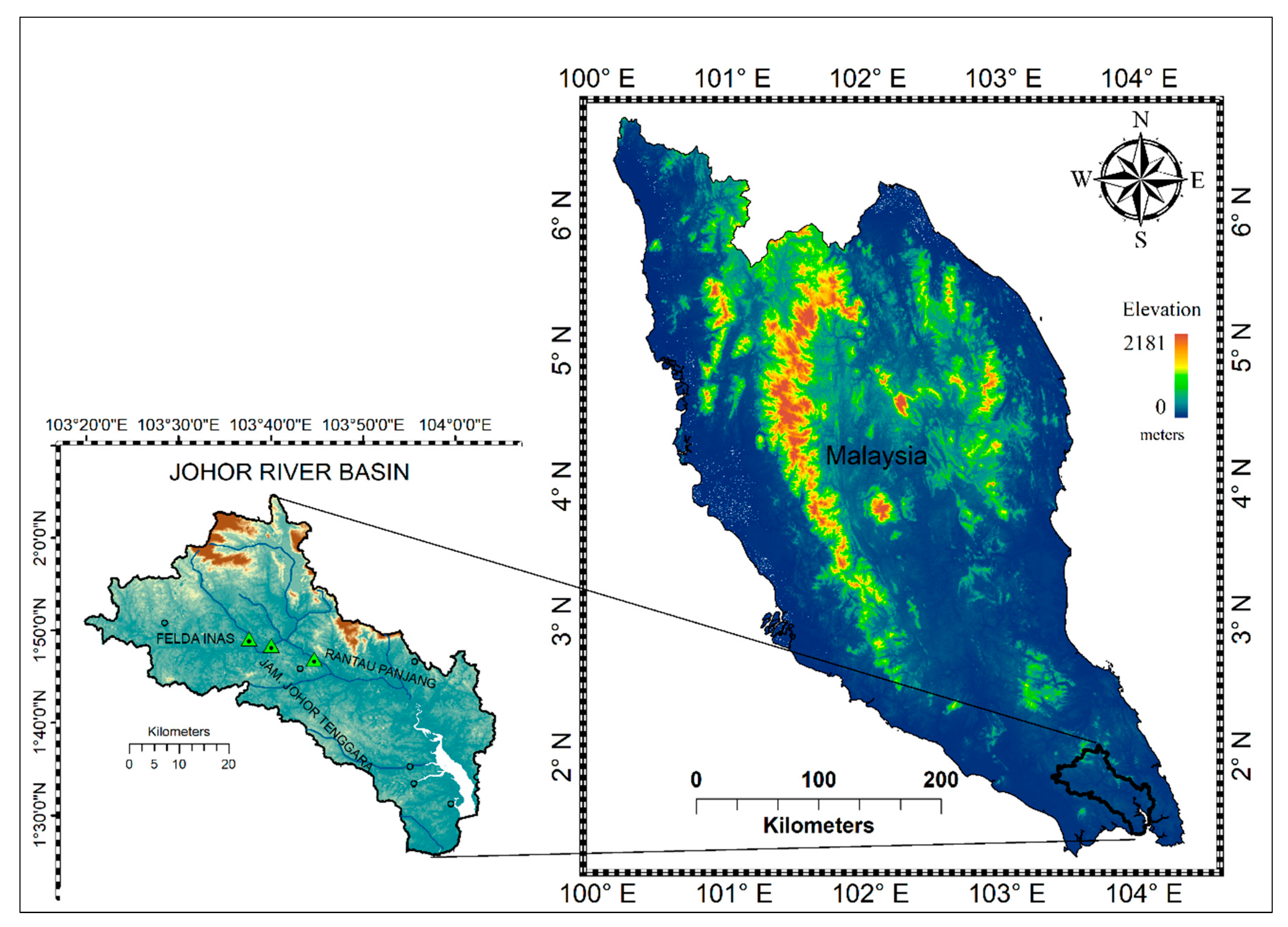
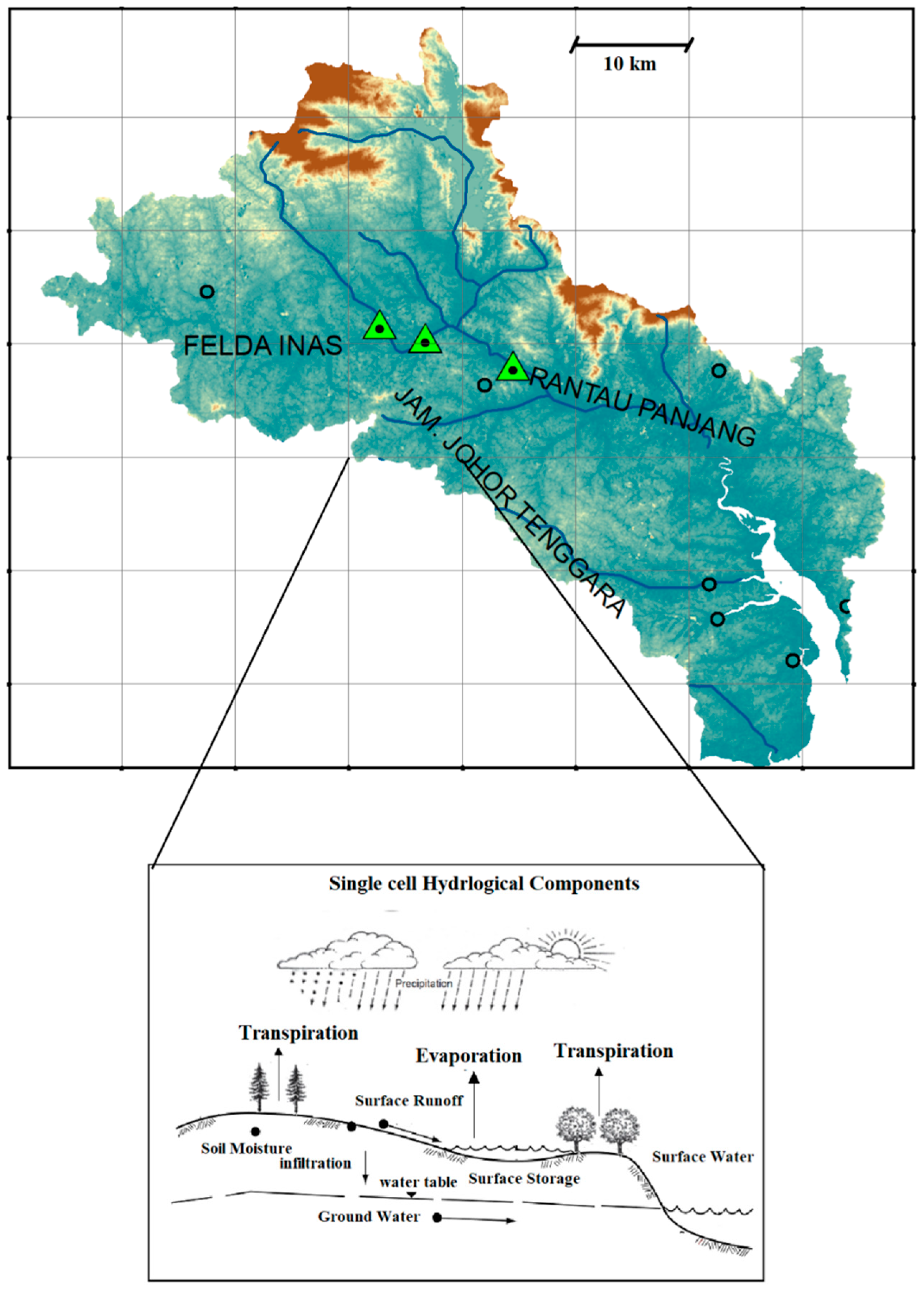
2.1. Study Area
2.2. Data Description
3. Methodology
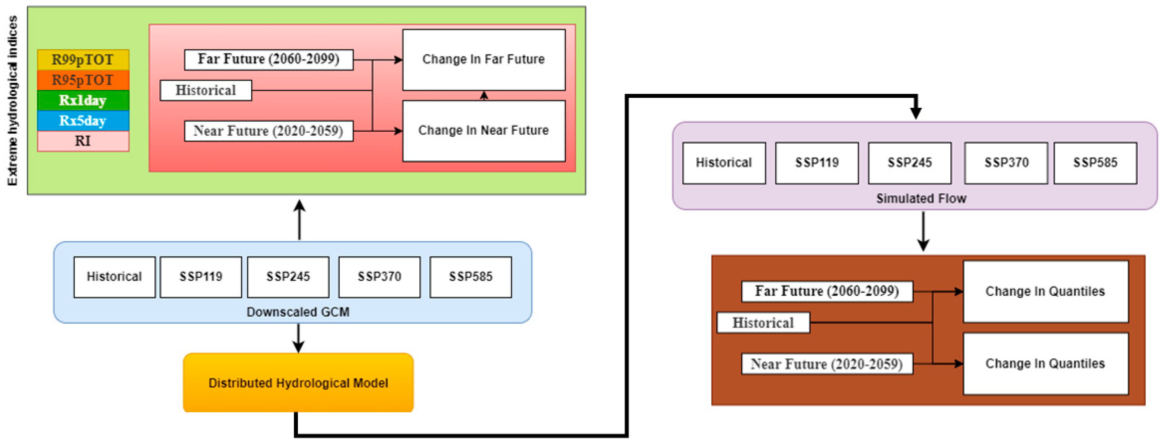
3.1. Procedure
- The catchment is divided into grids of 10 km each.
- All the data sets are interpolated to 10 km to achieve a similar resolution.
- The distributed hydrological model is developed using bias Corrected IMERG data for the catchment.
- The model is calibrated and validated with the observed river flow data (details given in Table 1).
- The selected GCMs are downscaled to 10 km resolution for the basin.
- The downscaled GCMs data is used in the distributed model to simulate the future flow condition under different SSP scenarios. The details of the methods used to complete the analysis are given below.
3.2. K-Nearest Neighbour
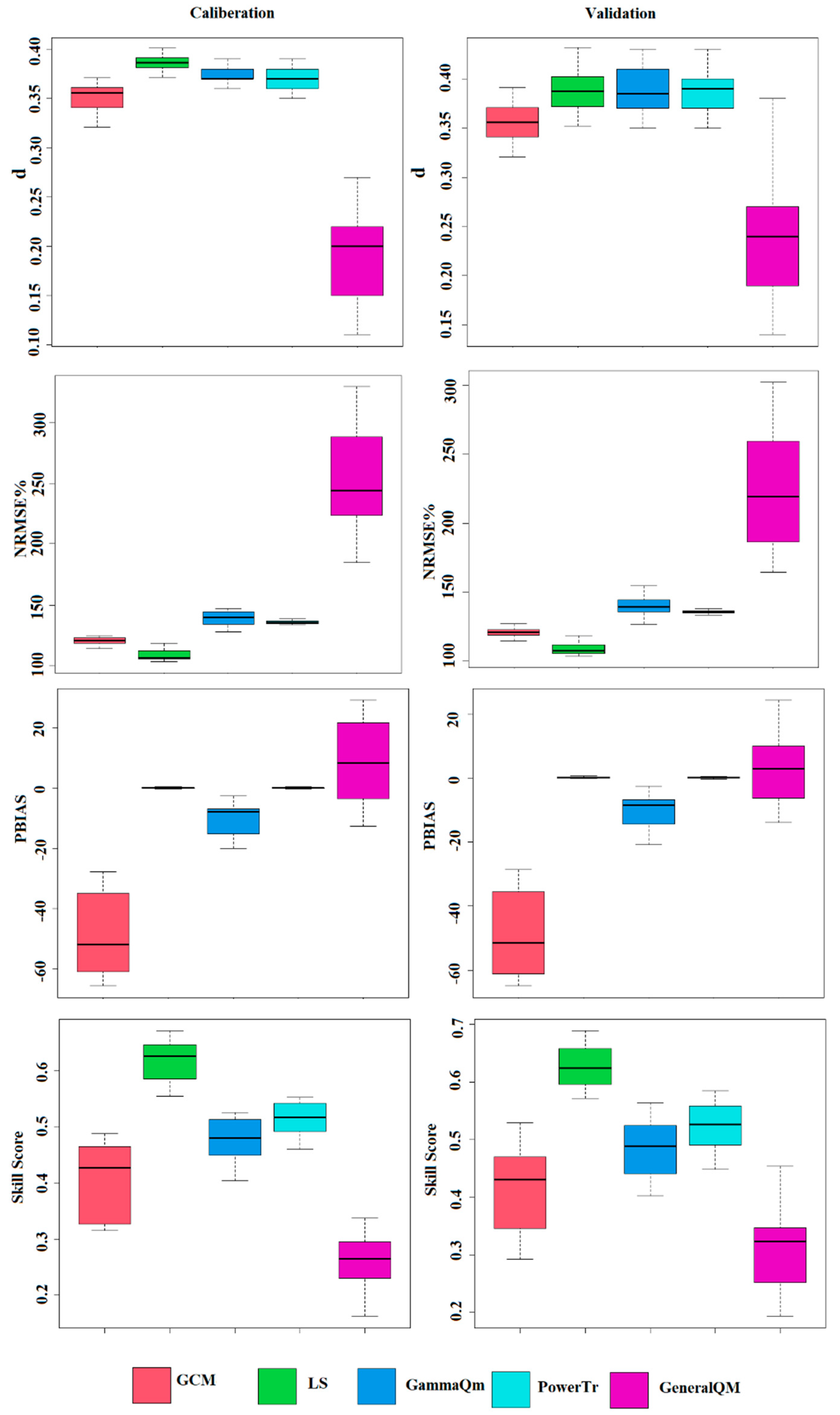
3.3. Downscaling of GCMs
3.3.1. Gamma Quantile Mapping
3.3.2. Power Transformation
3.3.3. Generalized Quantile Mapping
3.3.4. Linear Scaling
3.4. Hydrological Model Development
3.4.1. Concept of the Distributed Model
3.4.2. Excess Saturation Runoff Rate
3.4.3. Subsurface Runoff
3.4.4. Evapotranspiration
3.4.5. Flow Routing
- The average elevation of each grid is calculated for all the cells.
- The flow direction of each cell is calculated using the Eight Direction Pour point model.
- The flow accumulation in each cell is calculated using the bucket model developed in Section 3.3.1.
- Flow accumulation is calculated by adding the cumulated flow of the grids flowing into the particular grid
- The flow route is calculated by connecting the low water accumulated cells with high water accumulated cells.
3.4.6. Projections of Climate Change Impacts on Hydrological Extremes
4. Application Results
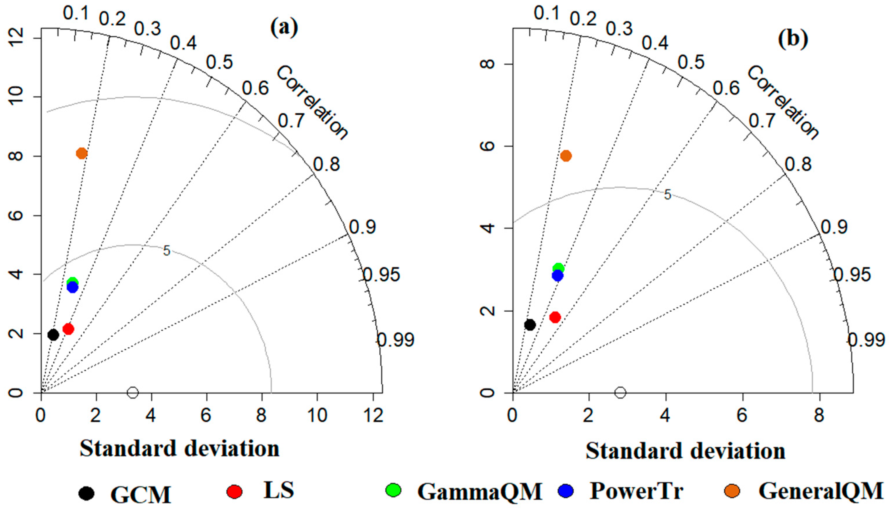
4.1. Downscaling of GCMs
4.1.1. Downscaling of Precipitation
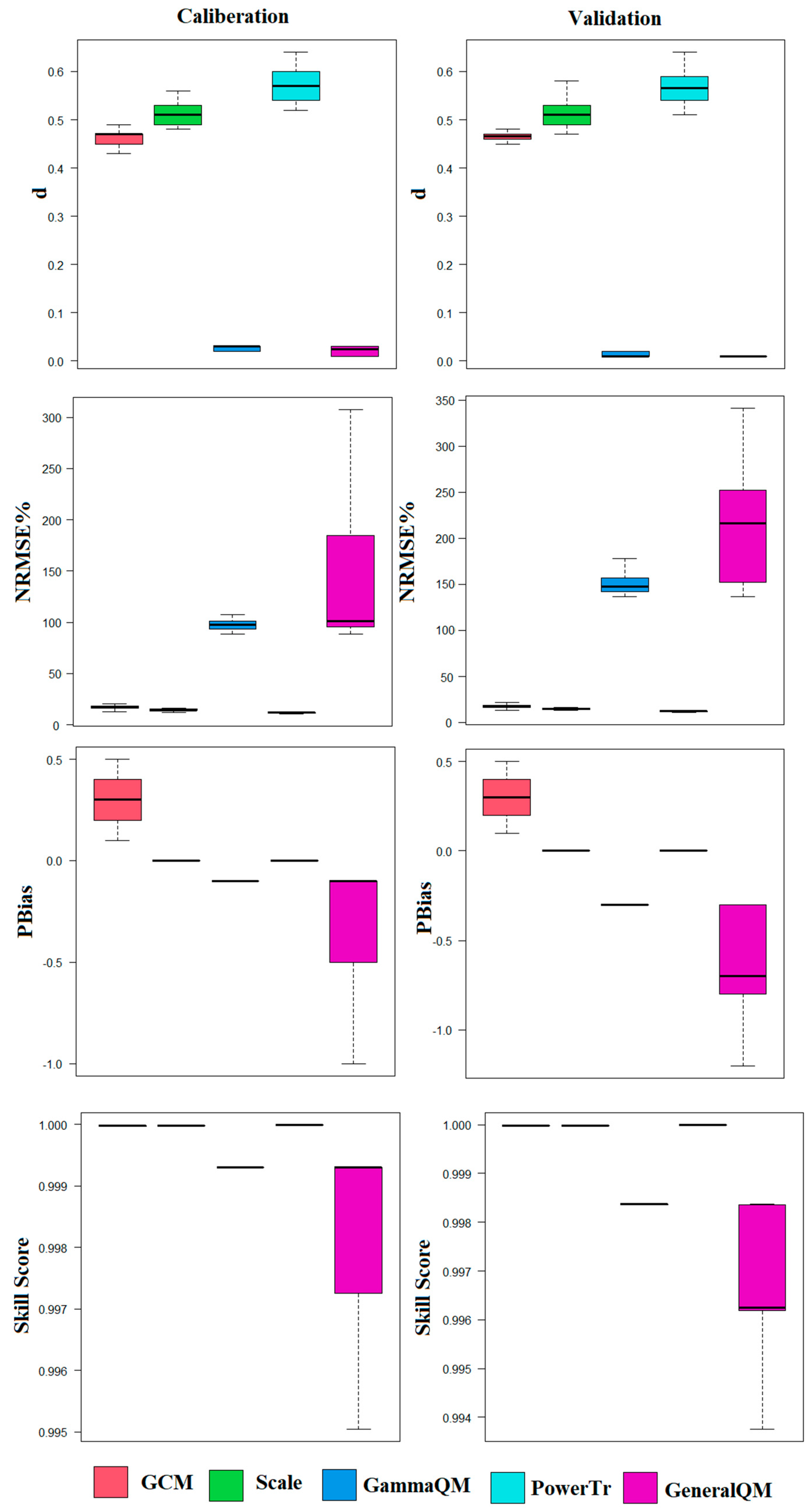
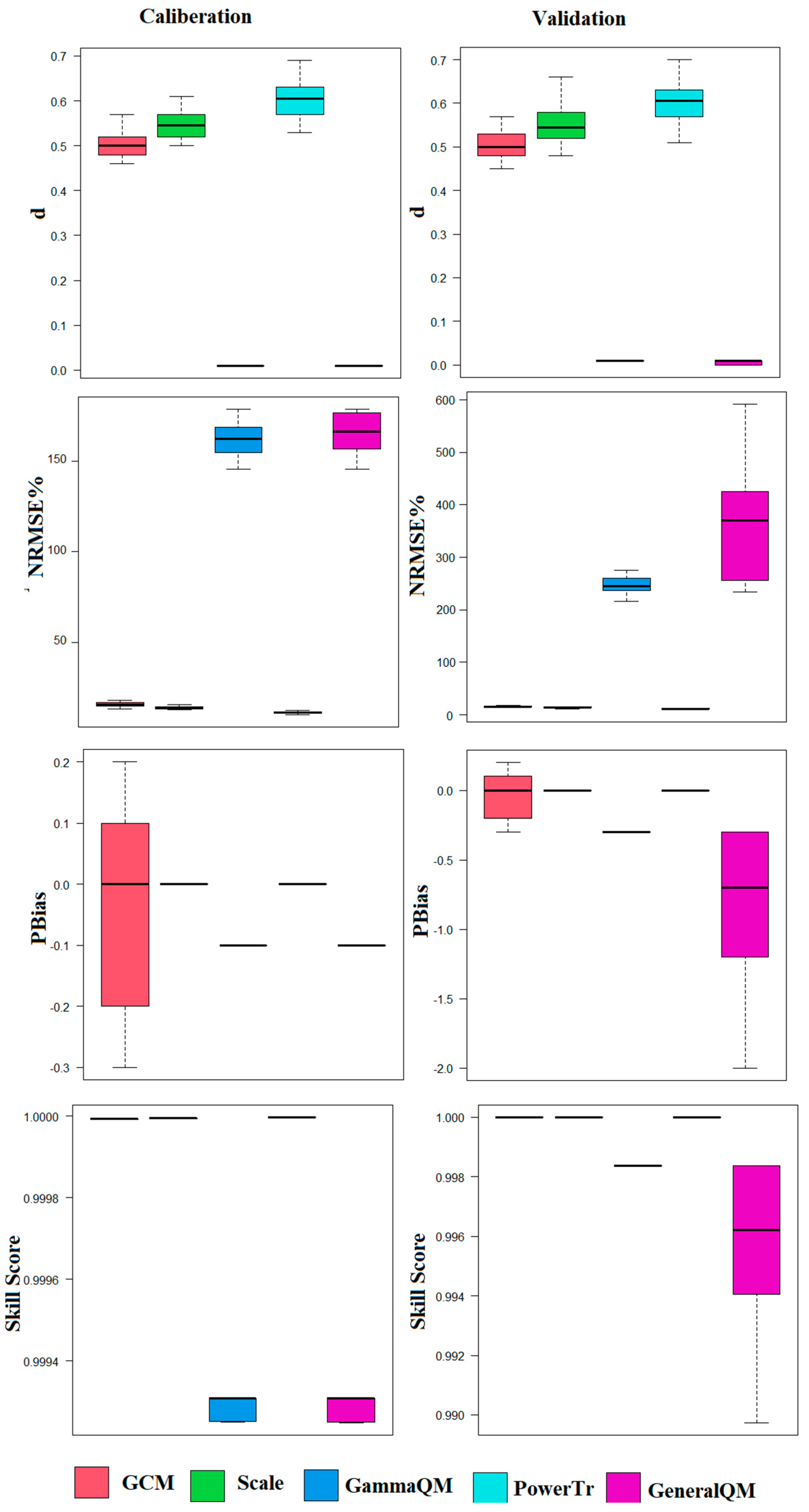
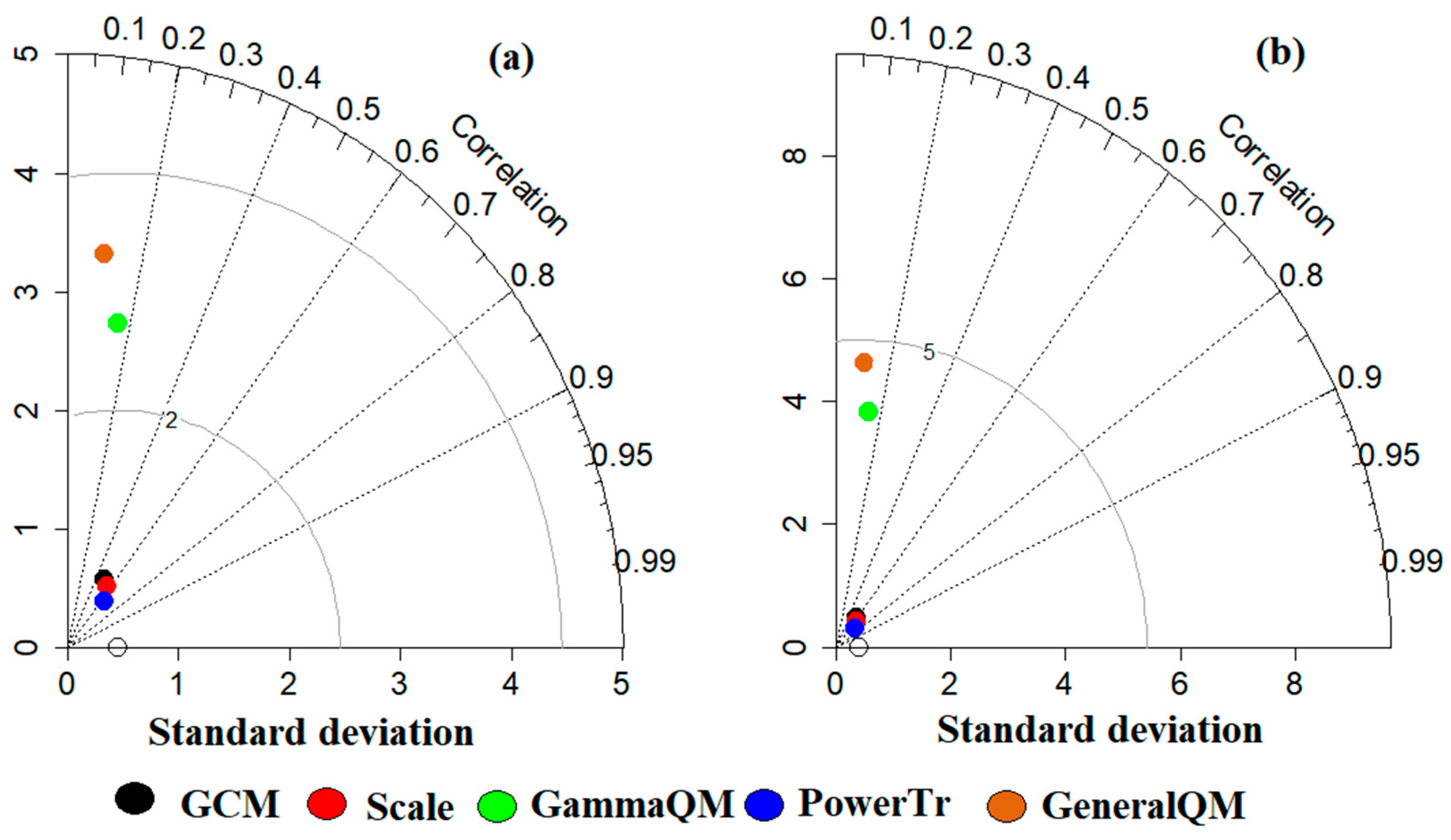
4.1.2. Downscaling of Maximum Temperature
4.1.3. Downscaling of Minimum Temperature
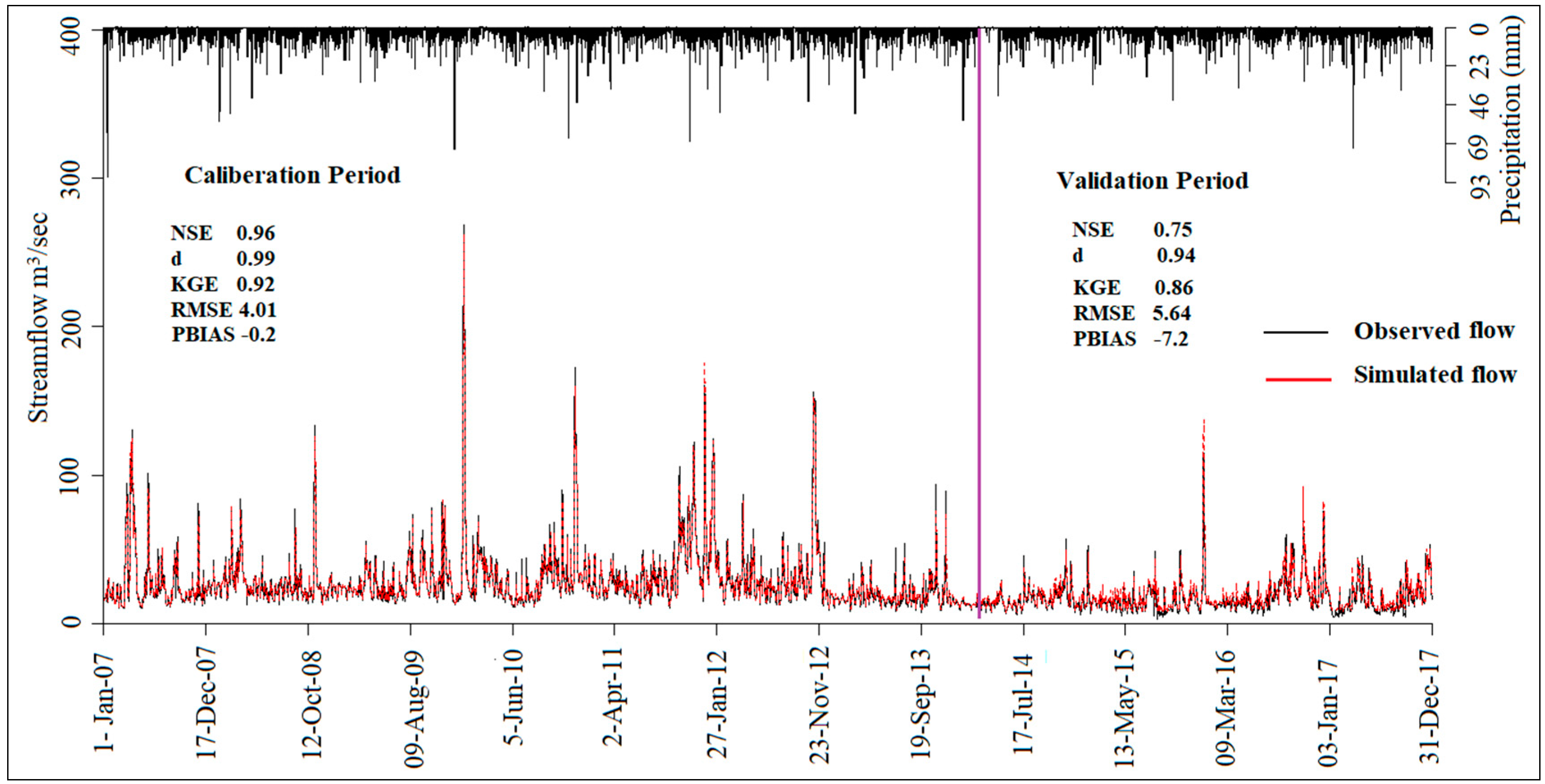
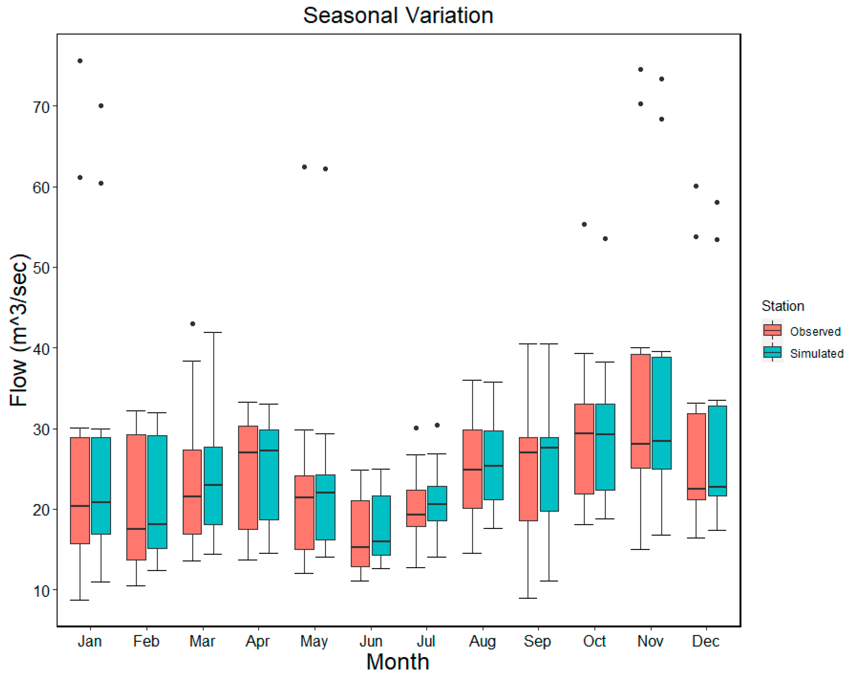
4.2. Calibration and Validation of Hydrological Model
4.3. Hydrological Changes under Future Scenarios
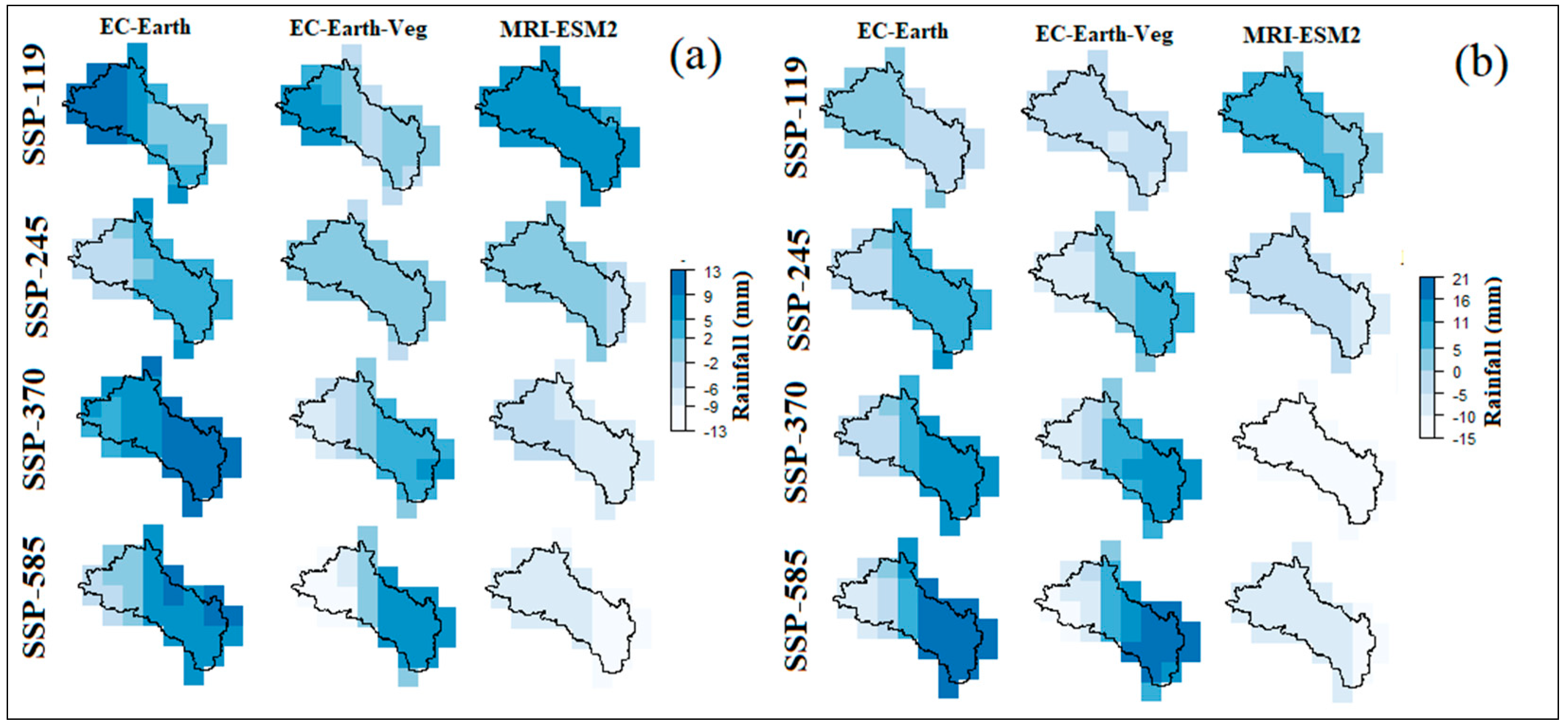
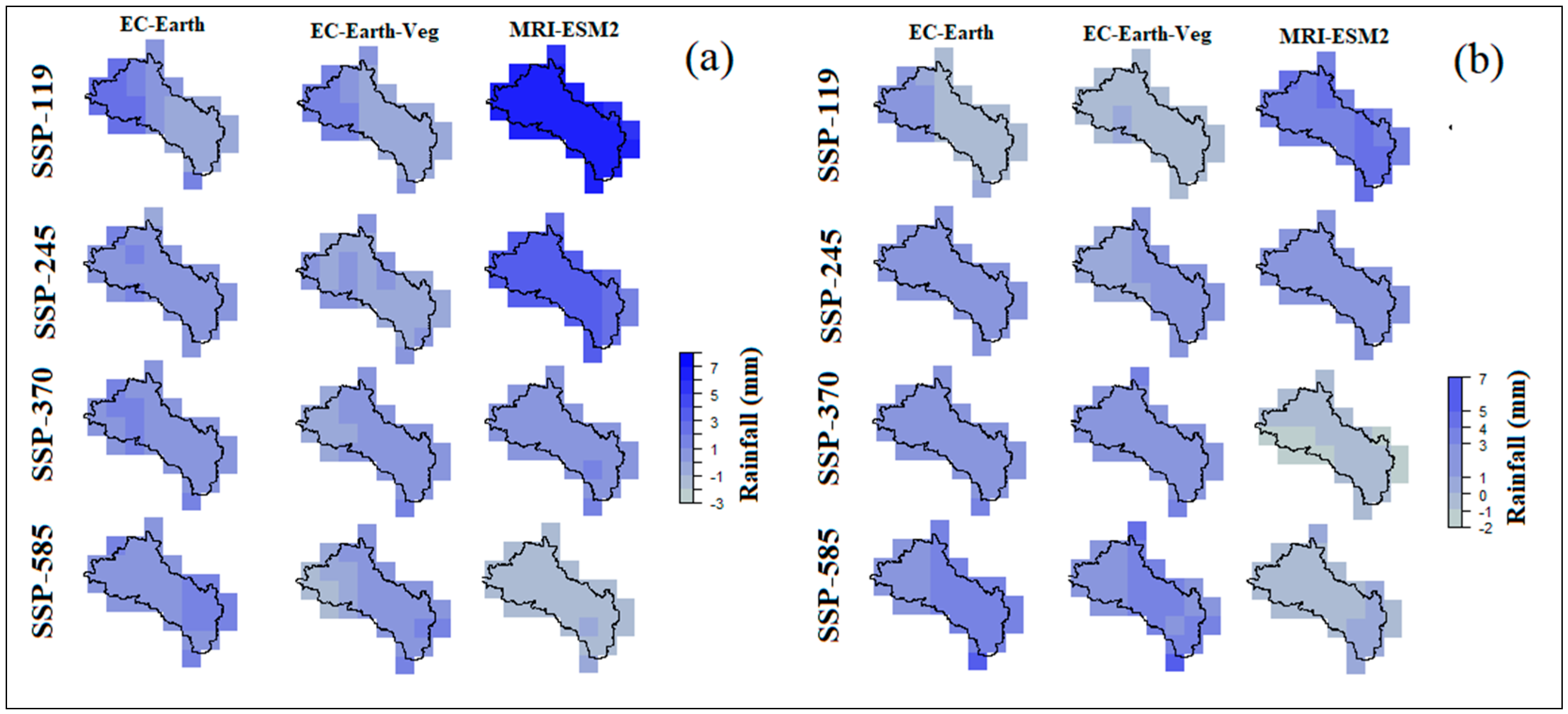
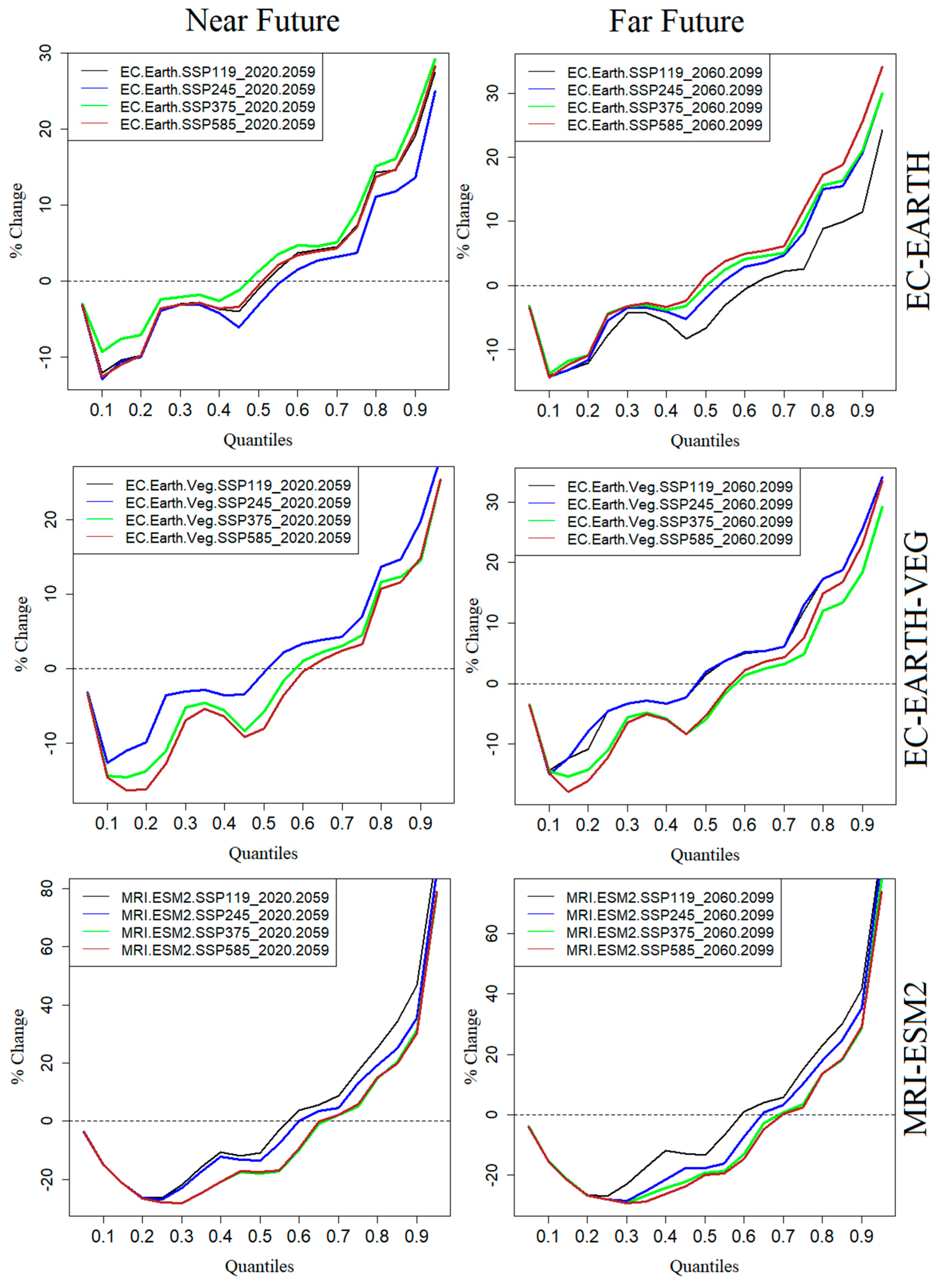
4.3.1. Projected Rainfall Extremes
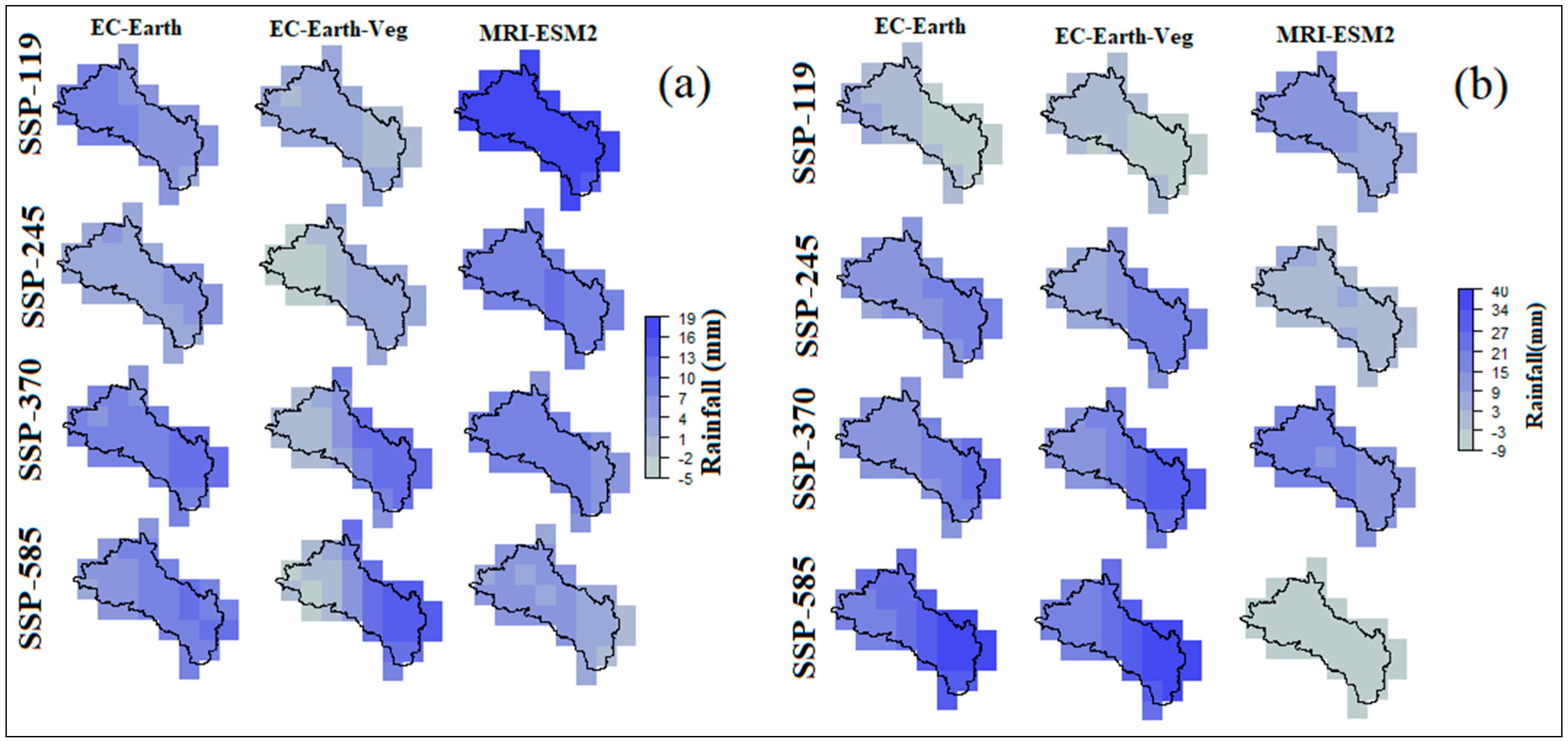
Total Rainfall above 95th Percentile (R95pTOT)
Total Rainfall above 99th Percentile (R99pTOT)
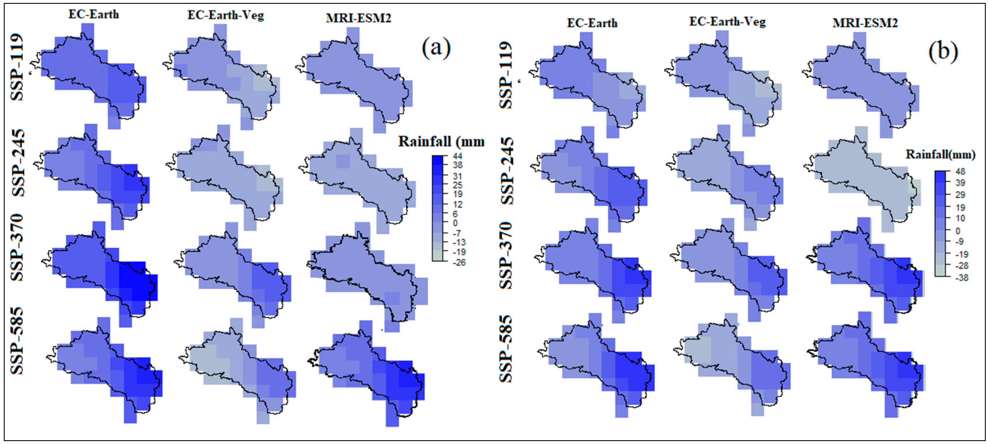
Changes in One Day Max Rainfall (R × 1day)
Changes in 5-Day Max Rainfall (R × 5day)
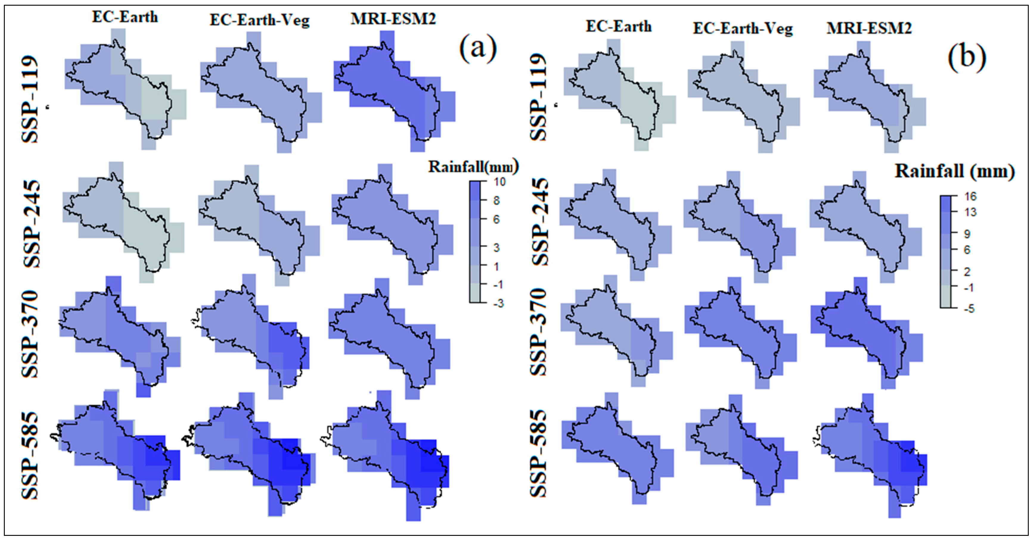
Changes in Rainfall Intensity (RI)
4.3.2. Changes in River Flow
5. Discussion
5.1. Reliability of the Newly Developed Model
5.2. Changes in Precipitation Flood Frequency under Future Scenario
5.3. Significance of the Study
6. Conclusions
Supplementary Materials
Author Contributions
Funding
Institutional Review Board Statement
Informed Consent Statement
Data Availability Statement
Acknowledgments
Conflicts of Interest
References
- Yaseen, Z.M.; Sulaiman, S.O.; Deo, R.C.; Chau, K.-W. An enhanced extreme learning machine model for river flow forecasting: State-of-the-art, practical applications in water resource engineering area and future research direction. J. Hydrol. 2019, 569, 387–408. [Google Scholar] [CrossRef]
- Vogel, R.M.; Lall, U.; Cai, X.; Rajagopalan, B.; Weiskel, P.K.; Hooper, R.P.; Matalas, N.C. Hydrology: The interdisciplinary science of water. Water Resour. Res. 2015, 51, 4409–4430. [Google Scholar] [CrossRef]
- Halder, B.; Haghbin, M.; Farooque, A.A. An Assessment of Urban Expansion Impacts on Land Transformation of Rajpur-Sonarpur Municipality. Knowl.-Based Eng. Sci. 2021, 2, 34–53. [Google Scholar] [CrossRef]
- Ahmad, S.; Simonovic, S.P. Spatial System Dynamics: New Approach for Simulation of Water Resources Systems. J. Comput. Civ. Eng. 2004, 18, 331–340. [Google Scholar] [CrossRef]
- Sa’adi, Z.; Shiru, M.S.; Shahid, S.; Ismail, T. Selection of general circulation models for the projections of spatio-temporal changes in temperature of Borneo Island based on CMIP5. Theor. Appl. Climatol. 2020, 139, 351–371. [Google Scholar] [CrossRef]
- Ehteram, M.; Othman, F.B.; Yaseen, Z.M.; Afan, H.A.; Allawi, M.F.; Malek, M.B.A.; Ahmed, A.N.; Shahid, S.; Singh, V.P.; El-Shafie, A. Improving the Muskingum flood routing method using a hybrid of particle swarm optimization and bat algorithm. Water 2018, 10, 807. [Google Scholar] [CrossRef] [Green Version]
- Sharafati, A.; Khazaei, M.R.; Nashwan, M.S.; Al-Ansari, N.; Yaseen, Z.M.; Shahid, S. Assessing the uncertainty associated with flood features due to variability of rainfall and hydrological parameters. Adv. Civ. Eng. 2020, 2020, 7948902. [Google Scholar] [CrossRef]
- Mango, L.M.; Melesse, A.M.; McClain, M.E.; Gann, D.; Setegn, S.G. Land use and climate change impacts on the hydrology of the upper Mara River Basin, Kenya: Results of a modeling study to support better resource management. Hydrol. Earth Syst. Sci. 2011, 15, 2245–2258. [Google Scholar] [CrossRef] [Green Version]
- Halder, B.; Ameen, A.M.S.; Bandyopadhyay, J.; Khedher, K.M.; Yaseen, Z.M. The impact of climate change on land degradation along with shoreline migration in Ghoramara Island, India. Phys. Chem. Earth Parts A/B/C 2022, 103135. [Google Scholar] [CrossRef]
- Saudi, A.S.M.; Juahir, H.; Azid, A.; Azaman, F. Flood risk index assessment in Johor River Basin. Malays. J. Anal. Sci. 2015, 19, 991–1000. [Google Scholar]
- Muzamil, S.A.H.B.S.; Zainun, N.Y.; Ajman, N.N.; Sulaiman, N.; Khahro, S.H.; Rohani, M.M.; Mohd, S.M.B.; Ahmad, H. Proposed Framework for the Flood Disaster Management Cycle in Malaysia. Sustainability 2022, 14, 4088. [Google Scholar] [CrossRef]
- Shahid, S.; Alamgir, M.; Wang, X.; Eslamian, S. Climate Change Impacts on and Adaptation to Groundwater. Handb. Drought Water Scarcity Environ. Impacts Anal. Drought Water Scarcity 2017, 2, 107–124. [Google Scholar]
- Ziarh, G.F.; Asaduzzaman, M.; Dewan, A.; Nashwan, M.S.; Shahid, S. Integration of catastrophe and entropy theories for flood risk mapping in peninsular Malaysia. J. Flood Risk Manag. 2021, 14, e12686. [Google Scholar] [CrossRef]
- Connor, R. The United Nations World Water Development Report 2015: Water for a Sustainable World; UNESCO Publishing: Bonn, Germany, 2015; Volume 1, ISBN 9231000713. [Google Scholar]
- Chemicals, U. Standardized Toolkit for Identification and Quantification of Dioxin and Furan Releases; United Nations Environment Programme: Geneva, Switzerland, 2003; Volume 194. [Google Scholar]
- Iqbal, Z.; Shahid, S.; Ahmed, K.; Ismail, T.; Nawaz, N. Spatial distribution of the trends in precipitation and precipitation extremes in the sub-Himalayan region of Pakistan. Theor. Appl. Climatol. 2019, 137, 2755–2769. [Google Scholar] [CrossRef]
- Ahmad, S.; Simonovic, S.P. System Dynamics Modeling of Reservoir Operations for Flood Management. J. Comput. Civ. Eng. 2000, 14, 190–198. [Google Scholar] [CrossRef]
- Sitterson, J.; Sinnathamby, S.; Parmar, R.; Koblich, J.; Wolfe, K.; Knightes, C.D. Demonstration of an online web services tool incorporating automatic retrieval and comparison of precipitation data. Environ. Model. Softw. 2020, 123, 104570. [Google Scholar] [CrossRef]
- Young, P.C. Advances in real–time flood forecasting. Philos. Trans. R. Soc. London. Ser. A Math. Phys. Eng. Sci. 2002, 360, 1433–1450. [Google Scholar] [CrossRef] [Green Version]
- Fahimi, F.; Yaseen, Z.M.; El-shafie, A. Application of soft computing based hybrid models in hydrological variables modeling: A comprehensive review. Theor. Appl. Climatol. 2017, 128, 875–903. [Google Scholar] [CrossRef]
- Naganna, S.R.; Beyaztas, B.H.; Bokde, N.; Armanuos, A.M. On the evaluation of the gradient tree boosting model for groundwater level forecasting. Knowl.-Based Eng. Sci. 2020, 1, 48–57. [Google Scholar] [CrossRef]
- Devia, G.K.; Ganasri, B.P.; Dwarakish, G.S. A Review on Hydrological Models. Aquat. Procedia 2015, 4, 1001–1007. [Google Scholar] [CrossRef]
- Perrin, C.; Michel, C.; Andréassian, V. Does a large number of parameters enhance model performance? Comparative assessment of common catchment model structures on 429 catchments. J. Hydrol. 2001, 242, 275–301. [Google Scholar] [CrossRef]
- Agrawal, N.; Desmukh, T.S. Rainfall Runoff Modeling using MIKE 11 Nam—A Review. Int. J. Innov. Sci. Eng. Technol. 2016, 3, 659–667. [Google Scholar]
- Yaseen, Z.M.; Ebtehaj, I.; Kim, S.; Sanikhani, H.; Asadi, H.; Ghareb, M.I.; Bonakdari, H.; Wan Mohtar, W.H.M.; Al-Ansari, N.; Shahid, S. Novel hybrid data-intelligence model for forecasting monthly rainfall with uncertainty analysis. Water 2019, 11, 502. [Google Scholar] [CrossRef] [Green Version]
- Khosravi, K.; Golkarian, A.; Booij, M.J.; Barzegar, R.; Sun, W.; Yaseen, Z.M.; Mosavi, A. Improving daily stochastic streamflow prediction: Comparison of novel hybrid data-mining algorithms. Hydrol. Sci. J. 2021, 66, 1457–1474. [Google Scholar] [CrossRef]
- Johari, A.; Javadi, A.A.; Habibagahi, G. Modelling the mechanical behaviour of unsaturated soils using a genetic algorithm-based neural network. Comput. Geotech. 2011, 38, 2–13. [Google Scholar] [CrossRef]
- Omeje, O.E.; Maccido, H.S.; Badamasi, Y.A.; Abba, S.I. Performance of Hybrid Neuro-Fuzzy Model for Solar Radiation Simulation at Abuja, Nigeria: A Correlation Based Input Selection Technique. Knowl.-Based Eng. Sci. 2021, 2, 54–66. [Google Scholar]
- Khan, N.; Shahid, S.; Juneng, L.; Ahmed, K.; Ismail, T.; Nawaz, N. Prediction of heat waves in Pakistan using quantile regression forests. Atmos. Res. 2019, 221, 1–11. [Google Scholar] [CrossRef]
- Wang, X.; Zhang, J.; He, R.; Amgad, E.; Sondoss, E.; Shang, M. A strategy to deal with water crisis under climate change for mainstream in the middle reaches of Yellow River. Mitig. Adapt. Strateg. Glob. Chang. 2010, 16, 555–566. [Google Scholar] [CrossRef]
- Qin, H.-P.; Su, Q.; Khu, S.-T. An integrated model for water management in a rapidly urbanizing catchment. Environ. Model. Softw. 2011, 26, 1502–1514. [Google Scholar] [CrossRef]
- Tidwell, V.C.; Passell, H.D.; Conrad, S.H.; Thomas, R.P. System dynamics modeling for community-based water planning: Application to the Middle Rio Grande. Aquat. Sci. 2004, 66, 357–372. [Google Scholar] [CrossRef]
- Ropero, R.F.; Rumí, R.; Aguilera, P.A. Modelling uncertainty in social–natural interactions. Environ. Model. Softw. 2016, 75, 362–372. [Google Scholar] [CrossRef]
- Yaseen, Z.M.; Shahid, S. Drought Index Prediction Using Data Intelligent Analytic Models: A Review. In Intelligent Data Analytics for Decision-Support Systems in Hazard Mitigation; Springer: Cham, Switzerland, 2020; pp. 1–27. [Google Scholar]
- Chandwani, V.; Vyas, S.K.; Agrawal, V.; Sharma, G. Soft computing approach for rainfall-runoff modelling: A review. Aquat. Procedia 2015, 4, 1054–1061. [Google Scholar] [CrossRef]
- Koch, J.; Demirel, M.C.; Stisen, S. The SPAtial EFficiency metric (SPAEF): Multiple-component evaluation of spatial patterns for optimization of hydrological models. Geosci. Model Dev. 2018, 11, 1873–1886. [Google Scholar] [CrossRef] [Green Version]
- Guo, H.C.; Liu, L.; Huang, G.H.; Fuller, G.A.; Zou, R.; Yin, Y.Y. A system dynamics approach for regional environmental planning and management: A study for the Lake Erhai Basin. J. Environ. Manag. 2001, 61, 93–111. [Google Scholar] [CrossRef] [Green Version]
- Sood, A. Integrated Watershed Management as an Effective Tool for Sustainable Development: Using Distributed Hydrological Models in Policy Making. Ph.D. Thesis, University of Delaware, Newark, NJ, USA, 2009. [Google Scholar]
- Minville, M.; Cartier, D.; Guay, C.; Leclaire, L.-A.; Audet, C.; Le Digabel, S.; Merleau, J. Improving process representation in conceptual hydrological model calibration using climate simulations. Water Resour. Res. 2014, 50, 5044–5073. [Google Scholar] [CrossRef]
- Bárdossy, A.; Singh, S.K. Robust estimation of hydrological model parameters. Hydrol. Earth Syst. Sci. 2008, 12, 1273–1283. [Google Scholar] [CrossRef] [Green Version]
- Zhang, L.; Nan, Z.; Xu, Y.; Li, S. Hydrological Impacts of Land Use Change and Climate Variability in the Headwater Region of the Heihe River Basin, Northwest China. PLoS ONE 2016, 11, e0158394. [Google Scholar] [CrossRef] [Green Version]
- Zomorodian, M.; Lai, S.H.; Homayounfar, M.; Ibrahim, S.; Fatemi, S.E.; El-Shafie, A. The state-of-the-art system dynamics application in integrated water resources modeling. J. Environ. Manag. 2018, 227, 294–304. [Google Scholar] [CrossRef]
- Ratnayeke, S.; van Manen, F.T.; Clements, G.R.; Kulaimi, N.A.M.; Sharp, S.P. Carnivore hotspots in Peninsular Malaysia and their landscape attributes. PLoS ONE 2018, 13, e0194217. [Google Scholar] [CrossRef] [Green Version]
- Kia, M.B.; Pirasteh, S.; Pradhan, B.; Mahmud, A.R.; Sulaiman, W.N.A.; Moradi, A. An artificial neural network model for flood simulation using GIS: Johor River Basin, Malaysia. Environ. Earth Sci. 2012, 67, 251–264. [Google Scholar] [CrossRef]
- Tan, M.L.; Ficklin, D.L.; Ibrahim, A.L.; Yusop, Z. Impacts and uncertainties of climate change on streamflow of the Johor River Basin, Malaysia using a CMIP5 General Circulation Model ensemble. J. Water Clim. Chang. 2014, 5, 676–695. [Google Scholar] [CrossRef]
- Webster, P.J.; Magaña, V.O.; Palmer, T.N.; Shukla, J.; Tomas, R.A.; Yanai, M.; Yasunari, T. Monsoons: Processes, predictability, and the prospects for prediction. J. Geophys. Res. Ocean. 1998, 103, 14451–14510. [Google Scholar] [CrossRef]
- Noor, M.; Ismail, T.B.; Shahid, S.; Ahmed, K.; Chung, E.-S.; Nawaz, N. Selection of CMIP5 multi-model ensemble for the projection of spatial and temporal variability of rainfall in peninsular Malaysia. Theor. Appl. Climatol. 2019, 138, 999–1012. [Google Scholar] [CrossRef]
- Zhang, W.; Villarini, G.; Scoccimarro, E.; Napolitano, F. Examining the precipitation associated with medicanes in the high-resolution ERA-5 reanalysis data. Int. J. Climatol. 2020, 41, E126–E132. [Google Scholar] [CrossRef]
- Iqbal, Z.; Shahid, S.; Ahmed, K.; Ismail, T.; Ziarh, G.F.; Chung, E.-S.; Wang, X. Evaluation of CMIP6 GCM rainfall in mainland Southeast Asia. Atmos. Res. 2021, 254, 105525. [Google Scholar] [CrossRef]
- Iqbal, Z.; Shahid, S.; Ahmed, K.; Wang, X.; Ismail, T.; Gabriel, H.F. Bias correction method of high-resolution satellite-based precipitation product for Peninsular Malaysia. Theor. Appl. Climatol. 2022, 148, 1429–1446. [Google Scholar] [CrossRef]
- Huang, M.; Lin, R.; Huang, S.; Xing, T. A novel approach for precipitation forecast via improved K-nearest neighbor algorithm. Adv. Eng. Inform. 2017, 33, 89–95. [Google Scholar] [CrossRef]
- Maraun, D.; Wetterhall, F.; Ireson, A.M.; Chandler, R.E.; Kendon, E.J.; Widmann, M.; Brienen, S.; Rust, H.W.; Sauter, T.; Themel, M.; et al. Precipitation downscaling under climate change: Recent developments to bridge the gap between dynamical models and the end user. Rev. Geophys. 2010, 48, 2009RG000314. [Google Scholar] [CrossRef]
- Eden, J.M.; Widmann, M. Downscaling of GCM-Simulated Precipitation Using Model Output Statistics. J. Clim. 2014, 27, 312–324. [Google Scholar] [CrossRef]
- Piani, C.; Haerter, J.O.; Coppola, E. Statistical bias correction for daily precipitation in regional climate models over Europe. Theor. Appl. Climatol. 2010, 99, 187–192. [Google Scholar] [CrossRef] [Green Version]
- Wilcke, R.A.I.; Mendlik, T.; Gobiet, A. Multi-variable error correction of regional climate models. Clim. Change 2013, 120, 871–887. [Google Scholar] [CrossRef] [Green Version]
- Amengual, A.; Homar, V.; Romero, R.; Alonso, S.; Ramis, C. A statistical adjustment of regional climate model outputs to local scales: Application to Platja de Palma, Spain. J. Clim. 2012, 25, 939–957. [Google Scholar] [CrossRef] [Green Version]
- Leander, R.; Buishand, T.A. Resampling of regional climate model output for the simulation of extreme river flows. J. Hydrol. 2007, 332, 487–496. [Google Scholar] [CrossRef]
- Terink, W.; Hurkmans, R.; Torfs, P.; Uijlenhoet, R. Bias correction of temperature and precipitation data for regional climate model application to the Rhine basin. Hydrol. Earth Syst. Sci. Discuss. 2009, 6, 5377–5413. [Google Scholar]
- Coles, S.; Bawa, J.; Trenner, L.; Dorazio, P. An Introduction to Statistical Modeling of Extreme Values; Springer: Cham, Switzerland, 2001; Volume 208. [Google Scholar]
- Lenderink, G.; Buishand, A.; Van Deursen, W. Estimates of future discharges of the river Rhine using two scenario methodologies: Direct versus delta approach. Hydrol. Earth Syst. Sci. 2007, 11, 1145–1159. [Google Scholar] [CrossRef]
- Lafon, T.; Dadson, S.; Buys, G.; Prudhomme, C. Bias correction of daily precipitation simulated by a regional climate model: A comparison of methods. Int. J. Climatol. 2013, 33, 1367–1381. [Google Scholar] [CrossRef] [Green Version]
- Allen, R.G.; Pruitt, W.O. FAO-24 Reference Evapotranspiration Factors. J. Irrig. Drain. Eng. 1991, 117, 758–773. [Google Scholar] [CrossRef]
- Moriasi, D.N.; Arnold, J.G.; Liew, M.W.V.a.n.; Bingner, R.L.; Harmel, R.D.; Veith, T.L.; Van Liew, M.; Bingner, R.L.; Harmel, R.D.; Veith, T.L. Model Evaluation Guidelines for Systematic Quantification of Accuracy in Watershed Simulations. Trans. ASABE 2007, 50, 885–900. [Google Scholar] [CrossRef]
- Jeong, J.; Kannan, N.; Arnold, J.; Glick, R.; Gosselink, L.; Srinivasan, R. Development and Integration of Sub-hourly Rainfall–Runoff Modeling Capability Within a Watershed Model. Water Resour. Manag. 2010, 24, 4505–4527. [Google Scholar] [CrossRef]
- Ahmed, K.; Shahid, S.; Chung, E.S.; Ismail, T.; Wang, X.J. Spatial distribution of secular trends in annual and seasonal precipitation over Pakistan. Clim. Res. 2017, 74, 95–107. [Google Scholar] [CrossRef]
- Nashwan, M.S.; Shahid, S. Spatial distribution of unidirectional trends in climate and weather extremes in Nile river basin. Theor. Appl. Climatol. 2019, 137, 1181–1199. [Google Scholar] [CrossRef]
- Ge, F.; Zhu, S.; Luo, H.; Zhi, X.; Wang, H. Future changes in precipitation extremes over Southeast Asia: Insights from CMIP6 multi-model ensemble. Environ. Res. Lett. 2021, 16, 24013. [Google Scholar] [CrossRef]
- Kharin, V.V.; Flato, G.M.; Zhang, X.; Gillett, N.P.; Zwiers, F.; Anderson, K.J. Risks from Climate Extremes Change Differently from 1.5 °C to 2.0 °C Depending on Rarity. Earth’s Future 2018, 6, 704–715. [Google Scholar] [CrossRef]
- Li, C.; Zwiers, F.; Zhang, X.; Li, G.; Sun, Y.; Wehner, M. Changes in Annual Extremes of Daily Temperature and Precipitation in CMIP6 Models. J. Clim. 2021, 34, 3441–3460. [Google Scholar] [CrossRef]
- Pereira, L.S.; Cordery, I.; Iacovides, I. Coping with Water Scarcity: Addressing the Challenges; Springer Science & Business Media: New York, NY, USA, 2009; ISBN 978-1-4020-9578-8. [Google Scholar]


| Station ID | Station Name | River Basin | Catchment Area (km2) | Analysis Period |
|---|---|---|---|---|
| 1737451 | SG. JOHOR at RANTAU PANJANG | Sg Johor | 1130 | 2007–2017 |
| Data Set | Resolution | Source | |
|---|---|---|---|
| Land use | MODTBGA (MODIS/Terra Thermal Bands Daily L2G-Lite Global 1km SIN Grid V006 | 1 km | https://lpdaac.usgs.gov/ (accessed on 13 June 2021) |
| Rainfall | MOD16A2 (MODIS/Terra Net Evapotranspiration 8-Day L4 Global 500 m SIN Grid V006) | 500 m | https://lpdaac.usgs.gov/ (accessed on 13 June 2021) |
| Land Surface Temperature | MOD11A1-MODIS/Terra Land Surface Temperature/Emissivity Daily L3 Global 1km SIN Grid | 1 km | https://lpdaac.usgs.gov/ (accessed on 14 June 2021) |
| Elevation | ALOS/PALSAR DEM 12.5 m | 12.5 m | https://asf.alaska.edu/ (accessed on 19 July 2021) |
| Soil Type | SoilGrids250m version 2.0 | 250 m | https://soilgrids.org/ (accessed on 22 July 2021) |
| Indices | Symbol | Description | Formula |
|---|---|---|---|
| Total rainfall above 95th Percentile | R95pTOT | Annual total rainfall when rainfall > 95p | |
| Total Rainfall above 99th Percentile | R99pTOT | Annual total rainfall when rainfall > 99p | |
| One day Max Rainfall | R × 1day | Annual maximum 1-day rainfall | |
| Five-day Max Rainfall | R × 5day | Annual maximum 5-day rainfall | |
| Rainfall Intensity | RI | Average rainfall on the rainy days |
| MAE | RMSE | NRMSE% | Pbias | NSE | d | md | R2 | KGE | |
|---|---|---|---|---|---|---|---|---|---|
| Caliberation | 2.24 | 4.01 | 20.2 | −0.2 | 0.96 | 0.99 | 0.91 | 0.97 | 0.92 |
| Validation | 3.8 | 5.64 | 50.2 | −0.7 | 0.75 | 0.94 | 0.76 | 0.78 | 0.86 |
Publisher’s Note: MDPI stays neutral with regard to jurisdictional claims in published maps and institutional affiliations. |
© 2022 by the authors. Licensee MDPI, Basel, Switzerland. This article is an open access article distributed under the terms and conditions of the Creative Commons Attribution (CC BY) license (https://creativecommons.org/licenses/by/4.0/).
Share and Cite
Iqbal, Z.; Shahid, S.; Ismail, T.; Sa’adi, Z.; Farooque, A.; Yaseen, Z.M. Distributed Hydrological Model Based on Machine Learning Algorithm: Assessment of Climate Change Impact on Floods. Sustainability 2022, 14, 6620. https://doi.org/10.3390/su14116620
Iqbal Z, Shahid S, Ismail T, Sa’adi Z, Farooque A, Yaseen ZM. Distributed Hydrological Model Based on Machine Learning Algorithm: Assessment of Climate Change Impact on Floods. Sustainability. 2022; 14(11):6620. https://doi.org/10.3390/su14116620
Chicago/Turabian StyleIqbal, Zafar, Shamsuddin Shahid, Tarmizi Ismail, Zulfaqar Sa’adi, Aitazaz Farooque, and Zaher Mundher Yaseen. 2022. "Distributed Hydrological Model Based on Machine Learning Algorithm: Assessment of Climate Change Impact on Floods" Sustainability 14, no. 11: 6620. https://doi.org/10.3390/su14116620