Bi-Level Planning Model for Urban Energy Steady-State Optimal Configuration Based on Nonlinear Dynamics

Abstract

With the rapid development of social economy, energy consumption has continued to grow, and the problem of pollutant emissions in various energy sources has gradually become the focus of social attention. Cities account for two-thirds of global primary energy demand that make urban energy systems a center of sustainable transitions. This paper builds a bi-level planning model for steady-state optimal configuration to realize the reasonable planning of the urban energy structure. The first level mainly analyzes the steady-state relationship between energy systems, the second level is based on the steady-state relationship of multiple energy sources to minimize the construction and operating costs of urban energy systems and pollutant emissions. Nonlinear system dynamics and the Improved Moth Flame Optimization Algorithm (IMFO) algorithm are implemented to solve the model. In addition, this paper uses instances to verify the application of a planning model in a certain city energy system in China. Under the premise of ensuring the stability of the urban energy system, two energy planning programs are proposed: mainly coal or mainly high-quality energy. The coal planning volumes are used as the basis for sub-scenario planning and discussion. Lastly, this paper proposes a series of development suggestions for different planning schemes.

1. Introduction

Cities account for two-thirds of global primary energy demand that make urban energy systems a center of sustainable transitions [1]. Growing demands and technological shifts are changing global energy systems. For example, innovative technologies such as electric vehicles in the transport sector, and new equipment in the buildings sector, are projected to increase electricity demands in city areas. Cooling demands are the fastest growing in buildings, with subsequent extra load on electricity networks [2]. The Paris Climate Agreement added further traction to the growing international clout of cities as potent actors in both climate change mitigation and adaptation interventions [3]. At present, more than 50% of the world’s population lives in city areas, and this number is expected to rise to 70% by 2050 [4].

As is shown in Figure 1, the impact of economic activities on cities could be decomposed into scale effect, structure effect, and technology effect [5]. Firstly, the increase of economic aggregate is accompanied by more resource input and energy consumption, which also produces more environmental pollutants and has a negative effect on the environment, which is called scale effect. The change of productivity is often accompanied by the optimization of economic structure, which is reflected in the more reasonable allocation of resources and other factors, and has a positive effect on the environment, which is the structural effect. Secondly, with the development of economy, the optimization and upgrading of industrial structure is often reflected in the transformation and upgrading of energy-intensive heavy industry, and the vigorous development of service industry including high-tech industry, to promote the sustainable development of cities. Therefore, city areas have the potential to contribute significantly to global CO₂ emissions reductions through careful urban energy systems planning and community participation.

In recent years, with the rapid development of China’s social economy and the increasing improvement of people’s living standards, energy consumption has continued to grow, and the contradiction between energy supply and demand has become increasingly tense [6]. As the main body of energy production and consumption, cities play an important role in the strategy of energy revolution. However, the way of energy configuration is mainly the high pollution and high carbon emission, which is the lack of top-level design, planning integration, and action integration between energy and city development and between different energy sources [7]. An urban energy system refers to the use of advanced physical information technology to integrate coal, petroleum, natural gas, electric, thermal, and other energy sources in the region to achieve coordinated planning, optimized operation, and coordinated management among various heterogeneous energy subsystems. Under the dual pressures of economic development and environmental protection in cities of China, the reasonable planning and efficient operation of urban energy systems are the prerequisites for the rational use of urban energy, and it is also a hot spot at home and abroad [8]. Therefore, the main objectives of this paper are: (1) analyze the steady-state relationship between urban energy systems (coal, petroleum, natural gas, renewable energy); (2) establish an optimization model for urban energy planning based on the steady-state relationship of multiple energy sources to minimize the economic and environmental costs of urban energy systems, and provide a reference for top-level urban energy design.

The rest of this article is organized as follows. Section 2 introduces the literature review closely related to the establishment of urban energy system planning, identifies the main issues related to the methodological methods adopted, and illustrates the relevance and novelty of this research. Section 3 puts forward the typical structure of the urban energy system, and establishes a two-level programming model that considers the economic and environmental costs of the steady-state optimal allocation of urban energy. At the same time, some methods to solve the above models are proposed, including nonlinear system dynamics and IMFO. In Section 4, in order to verify the validity and rationality of the method proposed in this paper, the application of this model in the planning of a Chinese urban energy system is discussed and analyzed. Section 5 discusses some conclusions about the research; these conclusions are of great significance for readers to understand our research content and innovation.

2. Literature Review

The sustainable development of cities faces the triple dilemma of economic growth, energy sustainability, and environmental protection. A stable and reliable urban energy supply is essential to support economic growth and environmental protection. Therefore, many scholars have carried out extensive research on urban energy system planning, mainly focusing on three aspects: urban energy demand forecasting, urban energy system evaluation results, and related urban energy system planning technologies. In terms of urban energy forecasting, Yeo I A et al. [9] classified urban facilities according to the characteristics of energy use, and proposed a municipal energy demand prediction system composed of the e-gis database, energy planning database, and prediction algorithm. Yifei Y et al. [10] decomposed the influencing factors of energy demand into the economies of scale effect, population scale effect, energy structure effect, and household consumption effect based on the logarithmic average division index, and predicted China’s energy demand through the improved particle swarm optimization algorithm. Naiming X et al. [11] used the gray Markov prediction model to predict China’s energy demand while studying the self-sufficiency rate of China’s energy demand. Filippov S. P. et al. [12] considered the possible technical and structural changes in the future economy, the differences between different regions, the mutual substitution of energy carriers and energy conservation, separated economic variables from energy variables, and made a long-term prediction of urban energy demand. From the perspective of energy coupling, Weijie W et al. [13] proposed an energy demand prediction method based on Improved Gray Correlation Analysis and particle swarm optimization BP neural network, which effectively improved the prediction accuracy. Yanmeng Z [14] compared and analyzed the advantages, disadvantages, and applicable conditions of various energy demand prediction methods, and comprehensively used the idea of a combination model to construct a nonlinear combination prediction model of energy demand based on the Shapley value method and inclusive test.

Regarding the evaluation of the urban energy system, most scholars analyzed it from the aspects of reliability, sustainability, and stability. Rui J et al. [15] introduced ecological network analysis (ENA) as a general system analysis tool to simulate and evaluate urban energy supply security. The evaluation contents included the overall realizability evaluation, system attribute analysis, and structure analysis of the energy supply system. Chen C et al. [16] introduced the life cycle assessment (LCA) method to calculate the environmental impact load of different types of energy used in urban areas (including coal, petroleum, natural gas, and electricity), and evaluated the environmental impact of urban energy life cycle, which is helpful to realize the sustainable development of energy and environment. Kagaya S et al. [17] analyzed the urban energy system through fuzzy utility function and structural modeling, and evaluated the cost-effectiveness and environmental cost.

Based on the research results of urban energy demand and urban energy system evaluation, some scholars have also carried out wide research on urban energy system planning technology. Shan X et al. [18] selected and analyzed the typical commercial tools applicable to different cities by focusing on the planning and design of urban energy systems and energy consumption analysis tools. Xuyue Z et al. [19] proposed a modeling and optimization decision-making method for urban energy system transformation, focusing on the optimal configuration and operation to meet the energy demand. Considering the technical, social, economic, and environmental complexity of energy system. Neshat N et al. [20] developed a modeling framework based on a bilateral multi-agent to determine the best planning scheme of an energy system. Yazdanie M et al. [21] analyzed the gap between urban energy system modeling tools and methods, and developed an urban energy system modeling method considering social factors. Meirong S et al. [22] proposed a multi-objective optimization model at the urban sector scale to minimize energy consumption, energy costs, and environmental impact, and the life cycle assessment method is used to calculate the environmental impact caused by various pollutants in the chain of energy production, transportation, and consumption. Rexiang W et al. [23] established a Hamiltonian directed graph to describe the energy flow process between supply and demand in urban energy networks based on graph theory ideas, and proposed a multi-source, multi-sink, multi-path approach to planning urban energy systems.

Due to the lack of a scientific urban energy system planning method, there are still many problems in the planning process. For example, the management of a system is fragmented, and information between energy subsystems is not shared, therefore, the different energy systems focused on solving their own problems, which are lack of integrated optimization solutions for urban energy systems, etc. Therefore, there is an urgent need to carry out related research on the theory and technology of urban energy systems and multi-energy comprehensive planning, and establish a method for the steady-state optimization of urban energy systems. Ming S et al. [24] applied the C-D production function and the STIRPAT equation to construct an energy supply stability model based on nine factors affecting energy supply and demand. Aimin L et al. [25] quantified the development capacity, stability, and efficiency of the network in Tangshan City, China, from 2006–2016 using flow and informatization analysis of the ecological network analysis method. Xueting Z et al. [26] applied an improved ecological network analysis framework to study the internal metabolic processes and external stability of urban energy metabolic systems.

Nonlinear system dynamics is a discipline that studies the variation of state variables of a nonlinear system with time. In 1892, Russian scholar, Lyapunov, published the paper “General Problems of Motion Stability”, where he gave two methods to analyze the stability of ordinary differential equations. Among them, the first method of Lyapunov analyzed the local stability of the corresponding equilibrium point of the nonlinear system. kazaoka R [27] analyzed the power system stability of household users based on nonlinear dynamics, and obtained the mathematical model of power system. Hongshan Z et al. [28] projected the nonlinear power system dynamic model into a lower dimensional sub-space and proposed an empirical Gramian equilibrium reduction method for solving the nonlinear power system model reduction problem efficiently. Nonlinear influence relationships also exist between various types of urban energy sources, but there are still few studies on the application of this method to urban energy system stability, and scholars are needed to further construct urban energy system stability models and use nonlinear system dynamics to solve urban energy stability.

Therefore, in urban energy system planning, in order to clarify the advantages and disadvantages of the proposed model, this paper compares the existing typical research results from the aspects of research object, goal, and solving algorithms, whether it is bi-level, qualitative analysis, or quantitative analysis. The comparison results are shown in

Table 1. Comparison with several related papers.

Ref.	Research Object	Bi-Level	Objectives	Solving Algorithm	Qualitative/Quantitative
[9]	Electricity, heat	No	Minimum urban electricity demand	Urban energy demand forecasting algorithm	Quantitative
[10]	Influencing factors of energy demand	No	Minimum system cost	PSO-LSSVR	Quantitative
[11]	Natural gas, crude petroleum	No	Minimum system cost	A novel Markov approach based on quadratic programming model	Quantitative
[12]	Electric demand	No	Minimum annual total cost	EDFS computing system	Quantitative
[13]	Coal, petroleum, gas, and electricity	No	Minimum system cost	Improved particle swarm optimization	Quantitative
[14]	Coal, petroleum, natural gas, and renewable energy	No	Minimum system cost	Multiple linear regression, BP neural network	Qualitative and quantitative
[15]	Urban energy value system	No	Minimum system cost	Mixed integer linear programming	Quantitative
[16]	Coal, petroleum, natural gas, electricity, renewable energy	No	Minimum system cost	Life cycle assessment	Quantitative
[17]	Urban energy system	No	Minimum system cost	Fuzzy utility function	Qualitative
[18]	urban energy system planning and design tools	No	/	/	Qualitative
[19]	Urban energy equipment configuration planning	No	Minimum system cost	MINLP model and GAMS	Quantitative
[20]	Electricity	No	Maximum economic benefits	Technology learning mechanism	Quantitative
[21]	Urban energy system planning and modeling approaches	No	/	/	Qualitative
[22]	Coal, petroleum, natural gas, and electricity,	No	Minimum total energy cost, environmental impact, and total energy use	Life cycle assessment	Quantitative
[23]	Urban energy system	No	Maximum economic benefits	Hamiltonian directed graph	Qualitative and quantitative
[24]	Energy supply stability	No	Maximum urban energy system stability	Ridge regression analysis	Qualitative and quantitative
[25]	Urban energy system	No	/	Ecological network analysis	Qualitative and quantitative
[26]	Raw coal, coal products, and natural gas	No	/	Improved ecological network analysis framework	Qualitative and quantitative
[27]	Electric power system	No	/	Nonlinear dynamics	Qualitative
[28]	Power systems	No	/	Balanced empirical Gramian	Qualitative
This paper	Coal, petroleum, natural gas, and renewable energy	Yes	Minimum economic costs and environmental cost	Nonlinear system dynamics and IMFO	Qualitative and quantitative

below. It can be found that there are a lot of studies on urban energy systems and their planning, but there are still some unresolved problems: (1) In existing urban energy system planning, alternative relationships between different forms of energy are less considered, which may lead to repetitive planning; (2) Most existing planning models aim at the lowest system cost, but there is less consideration of the environment and whether the urban energy system is in a steady state at the optimal planning volume; (3) Most of the existing literature applies nonlinear system dynamics to solve mathematical or physical problems, with little extension to energy systems.

Based on these unresolved problems, this article established a bi-level planning model for urban energy steady-state optimal configuration. The main contributions of the paper are summarized as follows:

(1)

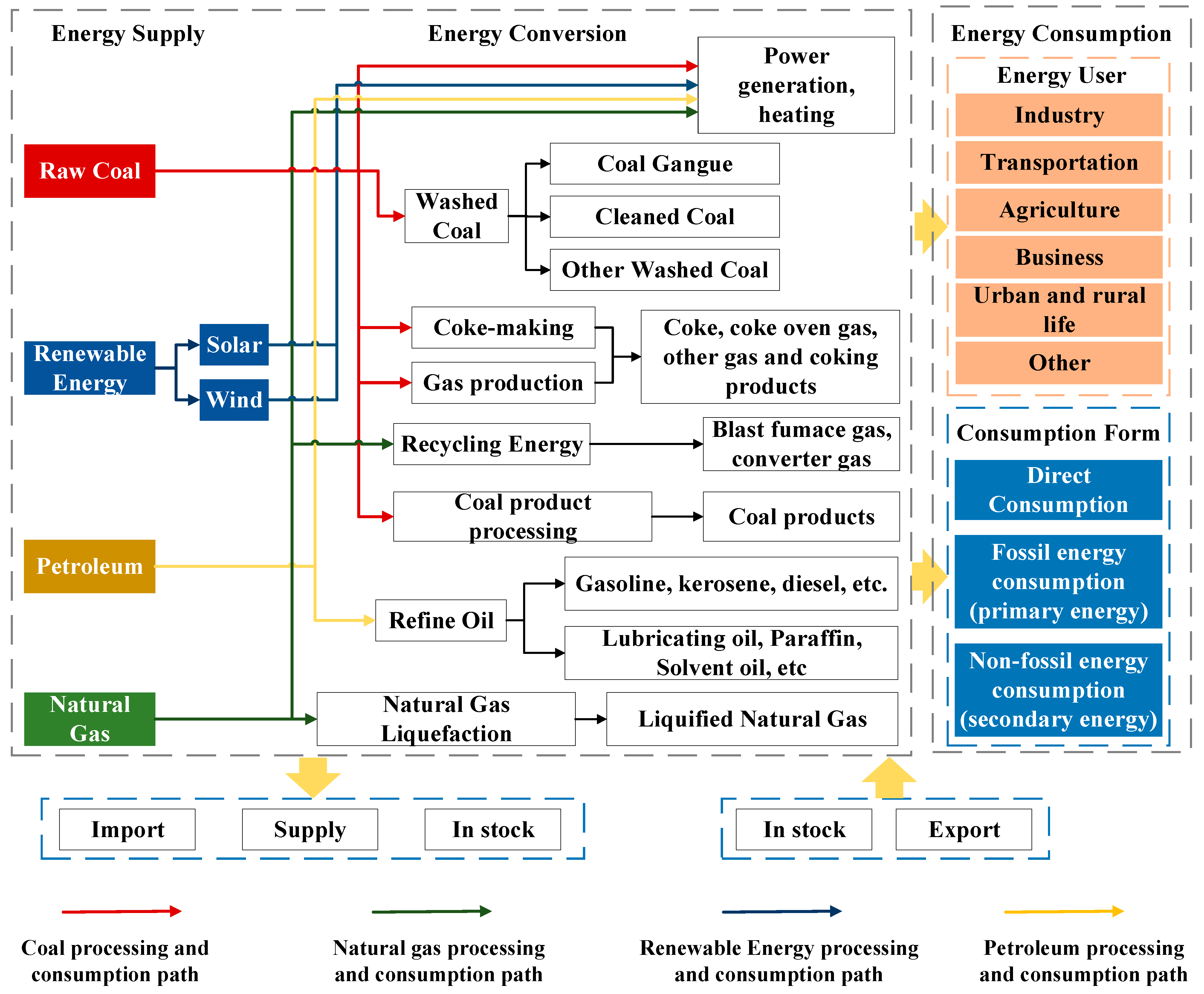
The basic structure of an urban energy system is built. Considering the substitution relationship between different energy forms, a bi-level optimization model of multi- energy comprehensive planning and steady-state configuration of urban energy system is proposed.

(2)

A four-dimensional nonlinear urban energy system model with coal as the main source and diversified development of natural gas, petroleum, and renewable energy is established, and the stability of nonlinear system solutions and Lyapunov’s theorem are applied to analyze the steady-state relationship of multiple energy sources and find out the demand for each energy source in the steady state of the urban energy system.

(3)

An urban energy system planning model is developed. Based on the steady-state relationship of multiple energy sources, the second-level planning model focuses on the energy planning configuration of the urban energy system in the steady state, to achieve the minimization of the construction and operation costs of the urban energy system, and as pollutant emissions petroleum.

3. Model of Bi-Level Programming

The urban energy system is an integrated system of energy production, processing conversion, and transmission allocation, which can realize the coordination and optimization of different energy sources in urban planning, construction, and operation. It mainly consists of three subsystems: energy supply system, energy conversion system, and energy consumption system. Figure 2 is a typical structural diagram of an urban energy system.

An urban energy system is an important concern for future energy development. The planning and allocation of urban energy is the key to urban economic operation. Aiming at the problem of urban energy steady-state optimal configuration, this paper establishes an bi-level programming optimization model for urban energy systems. The first level is a four-dimensional urban energy system model based on nonlinear system dynamics, which is used to find the demand for each energy source when the system is in a steady state. The optimization goal of the second level can be described as minimizing the economic cost and the environmental cost of the energy system under various constraints. The output results of the first-level model are the input parameters of the second-level model, which will affect the optimization results of the second-level model. Figure 3 is the bi-level optimization logic diagram of the urban energy system.

3.1. Four-Dimensional Nonlinear Urban Energy System Model of the First Level

In order to reduce consumption and optimize the urban energy structure, this paper established a nonlinear model that is dominated by coal and diversifies the development of natural gas, petroleum, and renewable energy (mainly including wind and photovoltaic). The model studies the interaction between the four to find out the demand for each energy source when the urban energy system is in a stable state. The objective function is:

$$F(x,y,z,r)=F_{balance-point}\{(x_1,y_1,z_1,r_1),(x_2,y_2,z_2,r_2),\dots ,(x_n,y_n,z_n,r_n)\}$$

(1)

where $X(t)$ is the coal consumption, $Y(t)$ is the natural gas consumption, $Z(t)$ is the petroleum consumption, $R(t)$ is the consumption of renewable energy (mainly including wind and photovoltaic). $(X,Y,Z,R)$ is the consumption of coal, petroleum, natural gas, and renewable energy under the constraints of each indicator when the urban energy system is in a stable state. In order to solve the consumption of energy in the urban energy system under steady state, a four-dimensional nonlinear urban energy system model X-Y-Z-R is established, as shown in Equation (2):

$$\{\begin{array}{l}\frac{dx}{dt}=a_{1}x\left(1-\frac{x}{M}\right)-a_2\left(y+z\right)-d_{3}r\\ \frac{dy}{dt}=b_{1}y+b_{2}x-b_{3}xz[N-(x+z)]\\ \frac{dz}{dt}=c_{1}z(c_{2}x-c_3)\\ \frac{dr}{dt}=d_{1}r-d_{2}x\end{array}$$

(2)

where $a_i,b_i,c_i,d_i,M$ are energy system steady-state coefficients and $a_i,b_i,c_i,d_i,M>0$ in the energy system, $a_1,b_1,c_1,d_1$ is the consumption elasticity coefficient of coal, natural gas, petroleum, and renewable energy, respectively; $a_2$ is the influence coefficient of petroleum and natural gas on coal, $b_2$ is the influence coefficient of coal on natural gas in the energy system, $b_3$ is the influence coefficient of coal and petroleum on consumption of natural gas in the energy system; $c_2$ is the price per unit of coal in the energy system and $c_3$ is the clean coal technology cost in the energy system; $d_2$ is the influence coefficient of coal, petroleum, and natural gas on renewable energy in the energy system and $d_3$ is the influence coefficient of renewable energy on coal in the energy system; M is the maximum energy gap and N is the threshold of environmental pollution in the energy system.

The model idea is as follows:

$a_{1}x\left(1-\frac{x}{M}\right)-a_2\left(y+z\right)-d_{3}r$ indicates that the coal consumption rate in the urban energy system is proportional to the energy gap and the potential gap share $1-X/M$ in the current energy system; the input of petroleum and natural gas reduces the demand gap of coal, and the utilization of renewable energy will reduce the demand for coal.

$b_{1}y+b_{2}x-b_{3}xz[N-(x+z)]$ indicates that a gap between the consumption rate of natural gas and itself; the ultimate return from coal can introduce more natural gas or vigorously develop coal-to-gas technology, thereby increasing the consumption of natural gas, therefore, the rate of natural gas consumption is directly proportional to the final return from coal; $-b_{3}xz[N-(x+z)]$ indicates that when the amount of environmental pollution generated by coal and petroleum in the urban energy system is less than the critical value ($(x(t)+z(t))<N$), the consumption rate of natural gas decreases with $x(t)$ and $z(t)$ increases, but when the amount of environmental pollution generated is greater than the critical value at the time ($(x(t)+z(t))>N$), since the amount of environmental pollution is controlled within the specified range, the consumption rate of natural gas increases with $x(t)$ and $z(t)$ increases.

$c_{1}z(c_{2}x-c_3)$ indicates that the consumption rate of petroleum is proportional to its own gap; at the same time, due to the final income generated by coal, more petroleum can be introduced or the coal-to-petroleum technology can be developed to increase the consumption of petroleum. Therefore, the rate of petroleum consumption is directly proportional to the final return from coal.

$d_{1}r-d_{2}x$ indicates that the consumption rate of renewable energy decreases with the increase of $x(t)$, and the consumption rate of renewable energy is proportional to its own gap.

3.2. Urban Energy System Planning Model of the Second Level

3.2.1. Objective Function

The goal of steady-state optimal allocation of urban energy systems is to minimize the economic cost of the energy system and minimize the amount of environmental pollution emissions during the planning period. Therefore, this paper proposes the optimal planning model including the economic scheduling model and the environmental scheduling model.

Before establishing the model, first establish the following assumptions: (1) the urban economy will maintain the development trend of growth and the future energy price can be reasonably predicted, and (2) the total energy consumption of the city in the future will not fluctuate violently.

• Economic model

The economic model only considers economic costs of power generation and energy supply. The cost of power generation technology is divided into two categories: fuel cost and operating investment cost. The cost of fuel is mainly the cost of coal, petroleum, and natural gas, which is included in the energy supply cost. The operating investment cost is included in the energy conversion cost. The energy conversion technology mainly refers to the power generation technology. The cost includes the operating costs and the investment costs of the newly-built units or the equipment.

$$\begin{array}{l}\min C_{\cos t}=C_s+C_c\\ =[P_{C,t}{L}_{C,t}+P_{NG,t}{L}_{NG,t}+P_{O,t}{L}_{O,t}+P_{RE,t}{L}_{RE,t}]+{\displaystyle \sum _t{\displaystyle \sum _k[C_{G(k,t)}{G}_{S(k,t)}+N_{G(k,t)}C(G_{k,t}^n)]}}\end{array}$$

(3)

where $C_{\cos t}$ is the total cost of the urban energy system; $C_s$ is the energy supply cost; $C_c$ is the energy conversion cost, t is the different period of the planning period; $P_{C,t},P_{NG,t},P_{O,t},P_{RE,t}$ is the price of coal, natural gas, petroleum, and renewable energy during the period t; $L_{C,t},L_{NG,t},L_{O,t},L_{RE,t}$ is the supply of coal, natural gas, petroleum, and renewable energy during the period t; $C_{G(k,t)}$ is the operating cost of local power generation technology k during the period t (power generation technology k includes coal power, gas power generation, wind power, solar power generation, etc.), $G_{S(k,t)}$ is the power generation capacity of local power generation technology k during the period t; $N_{G(k,t)}$ is the new capacity of local power generation technology k during the period t, and $C(G_{k,t}^n)$ is the unit investment cost of the new capacity of local power generation technology k during the period t.

2.

Environmental model

When the total amount of pollutant discharge does not exceed the maximum amount of pollutant discharge, the environmental cost is equal to the amount of each pollutant discharged from each source multiplied by its environmental price. When the total amount of pollutant discharge exceeds, the environmental cost includes the cost of excess penalty and the cost of ecological restoration.

$$C_e={\displaystyle \sum _{r=1}^R{K}_r{V}_r}+Z+G$$

(4)

where $C_e$ is the environmental cost; $K_r$ is the environmental value of the pollutant; $V_r$ is the pollutant emissions; $Z$ is the penalty cost due to excessive emissions, and $G$ is the cost of ecological restoration.

3.2.2. Constraint Conditions

Considering the factors affecting the urban energy system structure, the constraints of the second phase of the urban energy system include energy supply and demand balance constraint, energy exploitation capacity constraint, technical capacity constraint, energy planning policy constraint, and environmental constraint.

• Energy supply and demand balance constraint

Consider coal, petroleum, natural gas supply and demand balance constraints, and converted energy supply and demand balance constraints:

$$L_{S(n,t)}+I_{SM(n,t)}-E_{XS(n,t)}\ge D_{n,t}$$

(5)

where $L_{S(n,t)},I_{SM(n,t)},E_{XS(n,t)},D_{n,t}$ are the amount of production, purchase, consumption and forecast demand for energy n during the period t, respectively.

2.

Energy exploitation capacity constraint

$$L_{S(n,t)}\le {\beta }_{n,t}$$

(6)

where ${\beta }_{n,t}$ is the upper limit of the production capacity of energy n during the period t.

3.

Technical capacity constraint

$$L_{S(n,t)}\le G_{C(k,t)}{\overline{h}}_{k,t}(1-{\eta }_k)$$

(7)

where $G_{C(k,t)}$ is the upper limit of the installed capacity of the energy conversion technology k during the period t; ${\overline{h}}_{k,t}$ is the average annual running time of local power generation technology k during the period t, and ${\eta }_k$ is energy conversion technology update rate.

4.

Energy planning policy constraint

$$L_{S(n,t)}\le {\nu }_{n,t}$$

(8)

where ${\nu }_{n,t}$ is the upper limit of the supply capacity of energy n controlled in the government energy planning document during the period t.

5.

Environmental constraint

$$C_e=\{\begin{array}{cc}{\displaystyle \sum _{r=1}^R{K}_r{V}_r}& K_r\le K_{r-\max }\\ {\displaystyle \sum _{r=1}^R{K}_r{V}_r}+Z& K_r>K_{r-\max }\end{array}$$

(9)

where $K_{r-\max }$ is the maximum allowable emissions specified by environmental policy.

3.3. Model Solving Method

3.3.1. Solution of the First Level Based on Nonlinear System Dynamics

Nonlinear dynamic equations must express progressive laws. These nonlinear dynamic equations generally use ordinary differential equations containing time parameters. Nonlinear dynamic equations typically generally use regular differentials containing time parameters. The comparison or partial differential equation, i.e., the evolution equation, is defined, and the solution of the equation represents the motion of the system (how the state changes with time). The stability of the solution indicates whether the motion of the system is stable or not. Therefore, this article uses the stability of the nonlinear system solution and the Lyapunov theorem to study how urban energy changes over time.

• Dissipative analysis

$$\begin{array}{l}\nabla =\frac{\partial \dot{x}}{\partial x}+\frac{\partial \dot{y}}{\partial y}+\frac{\partial \dot{z}}{\partial z}=a_1-\frac{2a_{1}x}{M}-b_1+c_1{c}_{2}x-c_1{c}_3\\ =(c_1{c}_2-\frac{2a_1}{M})x+(a_1-b_1-c_1{c}_3)\end{array}$$

(10)

When $a_1-b_1<c_1{c}_3$$a_1-b_1<c_1{c}_3$ and $\frac{2a_1}{M}=c_1{c}_2$, the urban energy system is dissipative.

2.

Balance point stability

When $\frac{dx}{dt}=0$, $\frac{dy}{dt}=0$, $\frac{dz}{dt}=0$, $\{\begin{array}{l}{a}_{1}X\left(1-\frac{X}{M}\right)-a_2\left(Y+Z\right)=0\\ b_{1}Y+b_{2}Z-b_{3}X[N-(X-Z)]=0\\ c_{1}Z(c_{2}X-c_3)=0\end{array}$ gets three balance points: S₁(0, 0, 0), S₂(x₂, y₂, z₂), S₃(x₃, y₃, z₃), the solution equation is as follows:

$$\{\begin{array}{l}{x}_2=\frac{a_2{b}_{3}MN-a_1{b}_{1}M}{a_2{b}_{3}M-a_1{b}_1}\\ y_2=\frac{a_1{b}_3\left(M-N\right)\left(a_2{b}_{3}MN-a_1{b}_{1}M\right)}{{\left(a_2{b}_{3}M-a_1{b}_1\right)}^2}\\ z_2=0\end{array}$$

(11)

$$\{\begin{array}{l}{x}_3=\frac{c_3}{c_2}\\ y_3=\frac{\left[\frac{a_1}{a_2}\left(1-\frac{x_3}{M}\right)\left(b_3{x}_3-b_2\right)-b_3{x}_3+b_{3}N\right]x_3}{b_1+b_3{x}_3-b_2}\\ z_3=\frac{\frac{a_1{b}_1}{a_2}{x}_3\left(1-\frac{x_3}{M}\right)-b_{3}N{x}_3+b_3{x}_3^2}{b_1+b_3{x}_3-b_2}\end{array}$$

(12)

When $a_2{b}_{3}N>a_1{b}_1$, since M > N, then $a_2{b}_{3}M>a_1{b}_1$.

At this time $0<x_1<\frac{a_2{b}_{3}MN-a_1{b}_{1}N}{a_2{b}_{3}M-a_1{b}_1}=N$, $y_1=\frac{b_3}{b_1}{x}_1(N-x_1),y_1>0$.

When $\frac{c_3}{c_2}\ge N$, the urban energy system has two balance points $S_1$, $S_2$; when $\frac{c_3}{c_2}<N$, there are three balance points $S_1$, $S_2$, $S_3$.

(1)

For the balance point S₁(0, 0, 0), the coefficient matrix of the linear approximation system is

$$J_0=\left[\begin{array}{ccc}{a}_1& -a_2& -a_2\\ b_{3}N& -b_1& -b_2\\ 0& 0& -c_1{c}_3\end{array}\right]$$

(13)

The characteristic equation is $(c_1-c_3-\lambda )[\lambda -(a_1-a_3)](\lambda +b_1{b}_3)=0$.

The characteristic root of $J_0$ is:

$$\begin{array}{l}{\lambda }_1=-c_1{c}_3<0,\\ {\lambda }_{2,3}=\frac{a_1-b_1\pm \sqrt{{(b_1-a_1)}^2-4(a_2{B}_{3}N-a_1{b}_1)}}{2}\end{array}$$

(14)

This article assumes that when ${(b_1-a_1)}^2<4(a_2{B}_{3}N-a_1{b}_1)$, namely ${(a_1+b_1)}^2<4a_2{b}_{3}N$, the conclusions can be obtained as following:

When $a_1<b_1$, ${\lambda }_{2,3}$ is a pair of conjugate complex roots with negative genuine parts, so that the three characteristic roots ${\lambda }_1,{\lambda }_2,{\lambda }_3$ all have negative real parts, then the system is stable at S₃ (0, 0, 0). When $a_1>b_1$, ${\lambda }_{2,3}$ is a pair of conjugate complex roots with positive real parts, then S₃ (0, 0, 0) is the unstable point. When $a_1=b_1$, ${\lambda }_{2,3}=\pm i\omega$.

(2)

For the balance point S₂ (x₂, y₂, z₂)

$J_1=\left[\begin{array}{ccc}{a}_1(1-\frac{2x}{M})& -a_2& -a_2\\ b_3(N-2x)& -b_1& -b_2+b_{3}x\\ 0& 0& c_1(c_{2}x-c_3)\end{array}\right]$ can be obtained from its Jacobian matrix.

The characteristic equation is $(c_1-c_3-\lambda )[(a_3-a_1)-\lambda ](\frac{b_1{b}_2(a_1-a_3)M}{a_1}-b_1{b}_3-\lambda )=0$.

The characteristic roots are ${\lambda }_1=c_1-c_3$, ${\lambda }_2=a_3-a_1$, and ${\lambda }_3=\frac{b_1{b}_2(a_1-a_3)M}{a_1}-b_1{b}_3=b_1[b_{2}M(1-\frac{a_3}{a_1})-b_3]$.

If $a_1>a_3,c_1<c_3$, $\frac{b_2(a_1-a_3)M}{a_1}<b_3$, the three roots are all negative, then S₂ is the stable equilibrium point. If $a_1<a_3$ or $c_1>c_3$, there is at least one positive root, then S₂ is the unstable equilibrium point. If $a_1=a_3$ or $c_1=c_3$, there is at least one zero root, and S₂ is in a critical state, and the system produces a bifurcation.

(3)

For the balance point S₃(x₃, y₃, z₃)

By its Jacobian matrix

$$J_2=\left[\begin{array}{ccc}{a}_1(1-\frac{2x_2}{M})& -a_2& -a_2\\ b_3(N-2x_2+z_2)& -b_1& -b_2+b_3{x}_2\\ c_1{c}_2{z}_2& 0& 0\end{array}\right]$$

(15)

The characteristic equation can be obtained as

$$\begin{array}{l}(c_1-c_3-\lambda )\{(a_1-\frac{2a_{1}x}{M}-a_3-\lambda )[b_1(b_{2}x-b_3)-\lambda ]+a_2{b}_1{b}_{2}y\}\\ -a_2\{-b_1{b}_2{c}_{2}xy+c_{2}y[b_1(b_{2}x-b_3)]\}+a_2{c}_{2}y\lambda =0\end{array}$$

(16)

Let $a_1-\frac{2a_{1}x}{M}-a_3=A$, $b_1(b_{2}x-b_3)=b_1(b_2\frac{b_3}{b_2}-b_3)=B=0$, $c_1-c_3=C$, $a_2{b}_1{b}_{2}y=P$, $a_2\{-b_1{b}_2{c}_{2}xy+c_{2}y[b_1(b_{2}x-b_3)]\}=Q=-a_2{b}_3{b}_1{c}_{2}y$, $a_2{c}_{2}y\lambda =H$.

The original formula becomes ${\lambda }^3-(A+C){\lambda }^2+(AC+P-H)\lambda +(Q-PC)=O$.

3.3.2. Solution of the Second Level Based on IMFO

The non-free lunch optimization theorem shows that no single optimization algorithm can solve all optimization problems, and the Moth–Flame Optimization (MFO) algorithm [29] faces the same problem mentioned above. MFO is prone to premature convergence and falls into local optimum when dealing with complex function problems, so it needs to be improved to improve its performance. To further improve the convergence accuracy, in addition to considering the iteration stage the algorithm is in, the adaptation value of the moths during the iteration should be taken into account, i.e., a dynamic inertia weight adjustment strategy that is jointly determined with the iteration stage and the adaptation value of the moths is proposed. Gaussian variation is used to locally perturb some of the poorer individuals to improve the convergence speed of the algorithm. The Corsi variation strategy is used to enhance the diversity of the population and to suppress the premature convergence of the algorithm, and thus to achieve global optimization.

• Dynamic inertia weights [30]

The inertia weight parameter has an important impact on the global and local search of the algorithm. The size of the weights in the MFO algorithm determines the degree of influence of the flame individuals in the last iteration on the moth individuals in the current iteration. At the beginning of the iteration, a high global search capability is desired to explore new solution spaces and jump out of local extremes. Later in the iteration, emphasis is placed on local exploitation to speed up convergence and discover the exact solution. If the MFO algorithm uses linear decreasing inertia weights for complex high-dimensional functions, when the number of iterations is large, the amount of change of inertia weights per iteration is small, which will affect the function of the weight adjustment strategy. At the same time, with a single change pattern, it will be difficult for the moth to fly out after falling into the local optimum in the late iteration. Based on the above analysis, in addition to considering the iteration stage the algorithm is in, the adaptation value of the moth should also be taken into account, i.e., the weight size is determined by both the number of iterations and the adaptation value of the moth. The dynamic inertia weights $\omega$ are described as follows.

$${\omega }_{ij}=\frac{\exp \left(\frac{f(j)}{\mu }\right)}{2.4+(\exp (-f(j)/\mu ))iter}$$

(17)

where $\mu$ is the average fitness value of the first optimization process; $f(j)$ is the fitness value of the $j$ moth; $iter$ denotes the number of current iterations. For the very small value optimization problem, the function value corresponding to the moth optimization solution is set as the fitness value. $f(j)$ shows a nonlinear decreasing trend and $2.4+(\exp (-f(j)/\mu ))iter$ shows a nonlinear increasing trend as the number of iterations increases, so the weight $\omega$ shows a nonlinear decreasing trend with the increase of fitness value and the number of iterations.

The improved logarithmic helix function for the flame position update is shown in Equation (18).

$$S(M_i,F_j)=w_{ij}\times D_i\times e^{bt}\times \cos (2\pi t)+(1-{\omega }_{ij})\times F_j$$

(18)

where $M_i$ denotes the $i$ moth; $F_j$ denotes the $j$ flame; $D_i$ is the distance from the $i$ moth to the $j$ flame; $b$ is a constant defining the logarithmic helix; $t$ is a random number belonging to [−1, 1] indicating the proximity of the moth’s next position to the flame (t = 1 means closest to the flame and t = −1 means farthest from the flame). The dynamic inertia weights change nonlinearly and dynamically with the number of iterations and the fitness value, and the artificial moth gradually moves toward the flame with the better fitness value, which facilitates the performance improvement of the MFO algorithm.

2.

Gaussian variation mechanism [31]

Gaussian variation $Gaussian(\partial ,{\wp }^2)$ is introduced. Where $\partial$ denotes the mean; ${\wp }^2$ denotes the variance; $\partial =0$, ${\wp }^2=\left|X_{ij}^{\ast t}\right|$; $\left|X_{ij}^{\ast t}\right|$ denotes the absolute value of the global optimal moth of the population at $t$ iterations. The improved formula for $M_j$ generation is described as follows.

$$M_{new}^t=M_j^{\ast t}+Gaussian(\partial ,{\wp }^2)$$

(19)

The global optimal position after Gaussian variation, i.e., the global optimal solution, is obtained according to the above formula. Gaussian variation can produce new offspring near the original parents. With this property, the diversity of moths and flames can be increased to further improve the local search ability and convergence speed.

3.

Corsi variant strategy [32]

The MFO itself does not have the ability to jump out of the local optimum, which leads to a premature algorithm and poor convergence accuracy. In this paper, a Corsi variation approach is used. When the position of the moth stagnates during the iteration, the individual undergoes a Cauchy variation to continue to approach the global optimum, while the optimal individual in the moth population does not undergo a variation to ensure that the current optimum is not lost.

At each iteration, the Cauchy variation is computed by the Cauchy distribution function to produce a Cauchy variation matrix with a mean of 0, and a standard deviation of 1. The result is multiplied by each dimension of the moth to be mutated as the update step. The equation for updating the position after introducing the variation is shown in Equation (20).

$$X_{new}=\varpi ·Cauchy(1,0)·\left[D_i{e}^{bt}\cos (2\pi t)+F_j\right]$$

(20)

where $Cauchy(1,0)$ denotes the Corsi distribution of $\gamma =1,x_0=0$, $\varpi$ affects the range of Corsi variants, the update formula for $\varpi$ is $\varpi =\epsilon ·(u_a-u_b)$. where $\epsilon$ is a parameter that varies with the number of iterations; $u_a$ and $u_b$ denote the upper and lower bounds of the solution space, respectively. The range over which the moths perform the Corsi variation increases with the number of iterations, expanding a larger search space for the moths during the algorithm stagnation period, and thus increasing the population diversity.

The solution process of the improved moth–flame-based optimization algorithm constructed in this paper is shown in Figure 4. The solution process is as follows.

(1)

System initialization. Input system parameters: energy system steady-state coefficients, energy demand, energy prices, pollutant emissions, and environmental cost factors, etc.

(2)

Population initialization. Generate the initialized population P; population algebra $N_{gen}=1$, t = 1.

(3)

Simulation. Calculation of economic and environmental target values.

(4)

Location update. Updating dynamic inertia weights, performing Gaussian and Corsi variances, and generating offspring population Q.

(5)

Simulation calculation. Calculating the economic environmental target, artificial moth and artificial flame fitness values for population Q, and ranking them by fitness value.

(6)

Combination. Combining the current population P with the offspring population Q to obtain a population, calculating the dominance relationship and aggregation distance of each individual according to the fitness function, and Pareto ranking the individuals.

(7)

Termination condition. Judge the termination condition; if the termination condition is satisfied, output the optimal solution, economic cost, and environmental cost, otherwise, return to step 4.

Figure 4. Flow chart of the second level based on IMOA.

Figure 4. Flow chart of the second level based on IMOA.

4. Simulation

4.1. Parameters

This paper selects a region in China as the research object. At the end of 2021, the resident population of the region was 17.95 million, the urban population was 9.31 million, the urbanization rate was 51.86%, and the resident floating population was 4.94 million. In 2021, the region achieved a regional GDP of 997.513 billion yuan, an increase of 6.1% over the previous year at comparable prices. The total retail sales of social consumer goods was 1227.01 billion yuan. Urban energy is mainly coal, petroleum, natural gas, and renewable energy. In this paper, MATLAB software is used to simulate and evolve the results. Figure 5, Figure 6, Figure 7, Figure 8, Figure 9, Figure 10, Figure 11, Figure 12, Figure 13, Figure 14, Figure 15, Figure 16 and Figure 17 are drawn by MATLAB software.

• Input parameters of the first level

Figure 5 shows the consumption of coal, petroleum, natural gas, and renewable energy in a region in China during 2005–2021.

2.

Input parameters of the second level

In addition to the parameters mentioned above,

Table 2. Forecast value of energy price in the urban energy system.

Energy	Price
Coal (yuan/t standard coal)	839.98
Petroleum (yuan/t standard coal)	3009.04
Natural Gas (yuan/t standard coal)	2701.15
Renewable Energy (yuan/t standard coal)	Wind: 1410.89 Solar: 1856.44

shows the forecast value of energy price in an urban energy system and

Table 3. Pollutant emissions and environmental cost factors (Unit standard coal) [33].

Pollutants		SO2	NOx	CO2	CO
Emission	Coal (kg/t)	18	8	1731	0.26
	Natural Gas (kg/106m3)	11.6	0.0062	2.01	0
	Petroleum (kg/t)	12	10.1	1592	0.33
Environmental value (yuan/kg)		6.00	8.00	0.023	1.00

is the pollutant emissions and environmental cost factors. We estimate that the energy demand of the region in China in 2022 is 14,400 tons of standard coal.

4.2. The First Level Simulation

• Determination of parameters of the nonlinear system a₁ and M

The expression of the energy structure’s logistic model is $\frac{dX}{dt}=a_{1}X\left(1-\frac{X}{M}\right)$, where $X_0=X{|}_{t=0}$.

The solution is $\{\begin{array}{c}X=\frac{M}{1+(\frac{M}{X_0}-1)e^{-a_{1}t}}\\ X=X{|}_{t=o}\end{array}$.

To estimate the equation, let $\frac{M}{X_0}-1=e^{\xi },F=\ln \frac{M-X}{X}$. Transform the solution to obtain the following linear equation $F=\xi -a_{1}t$.

Estimate $\zeta ,a_1$ by the least-squares method. For the sample data $\left\{X_t;t=1,2,\dots ,17\right\}$, construct the variable $F_t=\ln \frac{M-X_t}{X_t}$ and determine the approximate range of the maximum energy gap $M$ of the urban energy system based on the sample data, and use the determination coefficient $R^2=1-\frac{{\displaystyle \sum (F_t-\overline{F})}}{{\displaystyle \sum {(F_t-\overline{F})}^2}}$ as the standard. Take points one by one, substitute $\left\{F_t\right\}$, calculate $\left\{F_t\right\}$ under different $M$ values, and estimate the parameters $\zeta ,a_1$.

According to the above-mentioned theoretical knowledge, the parameters $a_1$ and $M$ can be determined, and it is determined that the approximate value range of $M$ is $[1.1,1.8]$, and the regression analysis results of

Table 4. Regression analysis results.

M	1.1	1.2	1.3	1.4	1.5	1.6	1.7	1.8
R2	0.81503	0.845683	0.916619	0.855389	0.993331	0.995554	0.99678	0.996837
$\zeta$	−1.174	−0.791	−0.5343	−0.9564	−0.1711	−0.0312	0.0911	0.1253
$a_1$	0.1081	0.0778	0.0636	0.1333	0.0496	0.0456	0.0426	0.0466

are obtained.

2.

Identification and determination of other nonlinear system parameters

The other parameters in the four-dimensional nonlinear urban energy system are identified by the Forcal program. After the debugging error reaches 10⁻⁴, the results of the parameters obtained are as follows.

As can be seen from

Table 5. Parameter identification results.

$a_1$	$a_2$	$b_1$	$b_2$	$b_3$	$c_1$	$c_2$	$c_3$	$d_1$	$d_2$	$d_3$	$M$	$N$
0.0466	0.15	0.06	0.082	0.06	0.2	0.5	0.4	0.1	0.06	0.13	1.8	1

, when the fitting coefficient R² has the highest degree of fit, so it can be determined that $a_1$ is 0.0466. The three-dimensional view of the urban energy system is shown in Figure 6.

It can be seen from Figure 7 that in a short period, the elastic relationship of the energy sources $x(t),y(t),z(t),r(t)$ in the urban energy system is relatively stable. In the very beginning of evolutionary time, the elastic relationship of the four energy sources will fluctuate to some extent, but the magnitude of fluctuations decreases over time. Over a long period, the elastic inertia of each energy source in the urban energy system shows a relatively stable state: regular fluctuations within a specific range. Figure 7 shows that when $d_3=0.13$, the urban energy system $x(t),y(t),z(t),r(t)$ will stabilize after a period.

When $d_3=0.13$, to verify the accuracy of the model, the four-dimensional nonlinear model proposed in this paper is used to forecast the total energy demand in the region from 2012–2021, using 2011 data as the initial condition (total energy demand is equal to the sum of coal, natural gas, petroleum, and renewable energy demand), where the forecast results are compared with the actual energy consumption of the region, and the forecast results are derived using the STIRPAT model [24]. The comparison results are shown in Figure 8. The STIRPAT model decomposes energy consumption into the product of three factors: population size, affluence, and technology level. The coefficients of each variable are derived by partial differencing and ridge regression analysis of the model to obtain a regional energy consumption function and forecast the results.

As can be seen from Figure 8, there are surges and fluctuations in the actual energy consumption in the region. The four-dimensional nonlinear model is able to judge the stability of the energy system based on previous years’ consumption of four types of energy: coal, natural gas, petroleum, and renewable energy, predicting surges or drops in energy consumption when the energy system is less stable, and slight fluctuations in energy consumption when the energy system is more stable. The STIRPAT model predicts energy consumption based on the population, economy, and technology of the region. The population and economy of the region are generally in a steady increase, while the level of technology is difficult to improve in a short period of time, therefore, its prediction of energy consumption increases slowly year by year without any surge or fluctuation. The average error of the prediction results of the four-dimensional nonlinear model is about 0.059, while the average error of the prediction results of the STIRPAT model is about 0.154, therefore, the prediction of the four-dimensional nonlinear model proposed in this paper is more accurate.

4.3. The Second Level Simulation

In order to verify the applicability of the IMFO algorithm selected in this paper, the MFO algorithm and the improved moth–flame optimization algorithm (IMFO) are selected to compare the algorithm convergence, as shown in Figure 9.

Figure 9a,b are the convergence curves of the economic cost and environmental cost of different algorithms with the population size when the population size is 1000. It can be clearly seen that the MFO algorithm tends to fall into local optimum when solving the model established in this paper, and the IMFO algorithm has better global search ability and convergence performance, and can obtain better results.

The nonlinear system dynamic parameters calculated in the first level are used as the input parameters of the second level of urban energy planning. Since the two objectives of the lowest economic cost and the lowest environmental cost are mutually exclusive, 20 sets of feasible solutions can be obtained. Therefore, when analyzing the relationship between different energy sources and objective values, it is necessary to analyze both economic and environmental costs. The Pareto results are shown in Figure 10.

According to the simulation results of the first level, a feasible solution for the stability of multiple sets of energy combinations is obtained. Still, the difference between the advantages and disadvantages of different feasible solutions is obvious. In the second level, the IMOA algorithm is used for simulation. The result of the first level is used as the input value of the second level. Under the objective function conditions and various constraints that satisfy the minimum economic cost and environmental cost, the target value is better. The 20 sets of feasible solutions are analyzed for operational conclusions. The specific results are shown in

Table 6. Second level simulation results.

No.	Coal (10,000 Tons of Standard Coal)	Natural Gas (10,000 Tons of Standard Coal)	Petroleum (10,000 Tons of Standard Coal)	Renewable Energy (10,000 Tons of Standard Coal)	Economic Cost (Billion Yuan)	Environmental Cost (Billion Yuan)
1	0.602982133	0.322441807	0.018182392	0.554282462	441.3970003	72.76593041
2	0.531510779	0.363596454	0.017329108	0.600545082	395.0105866	84.32441609
3	1.223222143	0.084486551	0.000717157	0.520514905	737.6377162	176.0332609
4	1.23253118	0.083563165	0.000756146	0.629394813	743.4596253	192.4520151
5	1.225144883	0.082584003	0.000797321	0.730605559	739.2684847	189.8653556
6	1.207153448	0.083162826	0.000832799	0.809391871	728.6800754	150.5531197
7	1.179411369	0.086001846	0.000867776	0.881071872	712.2418522	140.2292337
8	1.142718874	0.091766228	0.000901193	0.945140393	690.4312409	132.3944984
9	1.097732662	0.100890899	0.000931912	1.001174452	663.6385144	127.3137253
10	1.031886602	0.11698691	0.000964226	1.058524505	624.3604742	121.5998734
11	0.955122458	0.138414925	0.00098856	1.102813626	578.5061408	117.4752378
12	0.431885409	0.400346589	0.016227261	0.624552446	330.6338092	193.6766361
13	0.307915537	0.430287245	0.014855649	0.623654008	250.4515677	186.1370679
14	0.030632606	0.452986089	0.011700065	0.553422303	70.5408957	159.933346
15	0.163769308	0.449337899	0.013225338	0.59653623	156.9980795	168.4352068
16	0.187650579	0.336434923	0.000835972	1.042430204	117.9765388	181.4745739
17	0.771152721	0.194787951	0.001005602	1.150942565	468.4142455	99.45308016
18	0.598403545	0.246772582	0.00098234	1.150005826	364.8346072	65.09821296
19	0.868065361	0.16467288	0.001002937	1.133707255	526.4402196	103.1215876
20	0.403222837	0.297291733	0.0009248	1.113912957	247.6206412	192.4216718

.

Since the optimization variables and the target dimensions are inconsistent, the above feasible solutions are normalized, and the processing results are shown in Figure 11. The share of various energy and economic and environmental costs in each scenario is clearly mapped out.

According to the proportion of coal in the energy structure, the 20 groups of planning results are divided into two categories, as shown in Figure 12. The first category is the energy planning model based on coal. Under this type of development model, coal accounts for more than 50%; the second category is an energy planning model based on high-quality energy. Under such development models, petroleum, natural gas, and renewable energy account for more than 50%.

4.4. Analysis Results and Discussion

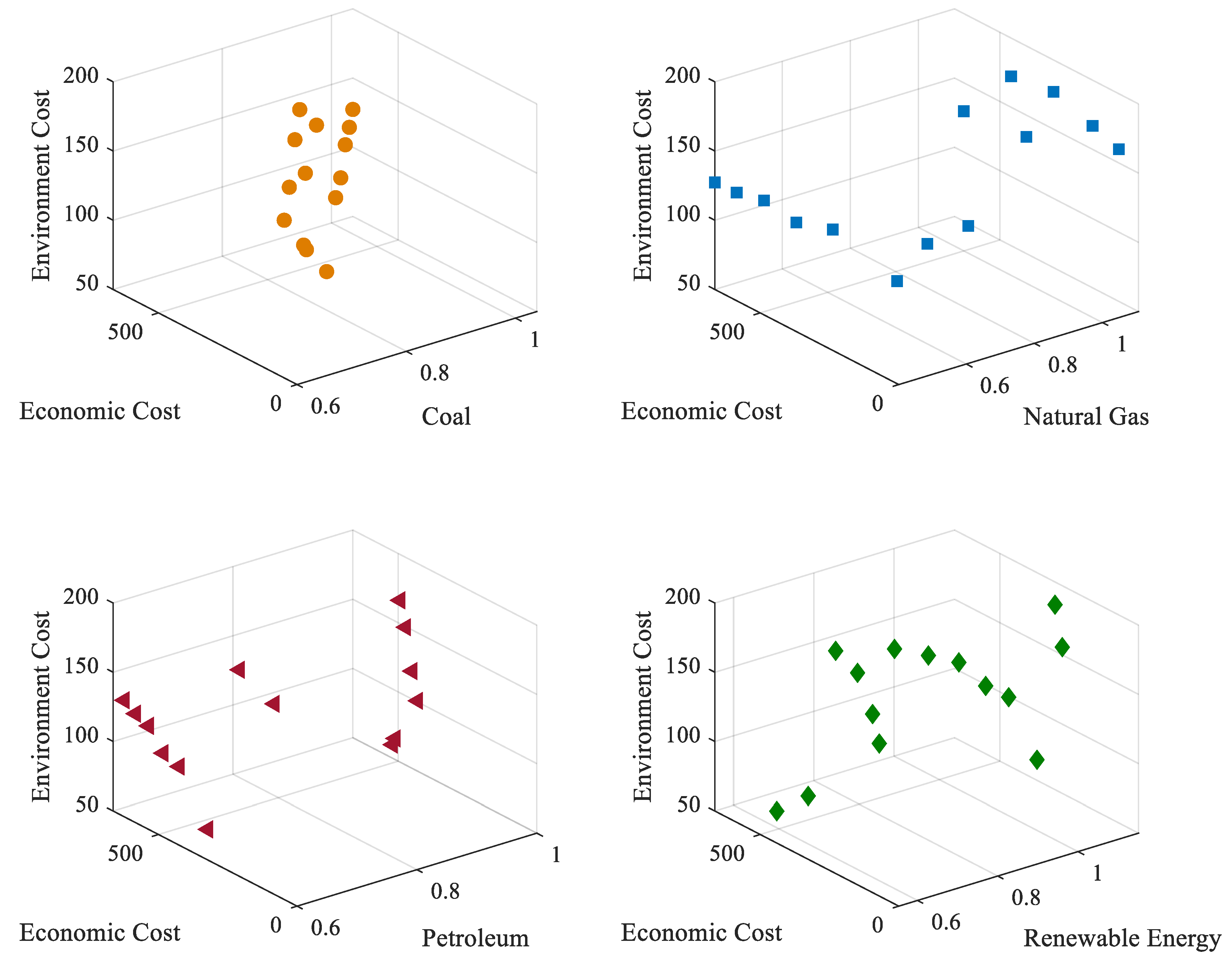
4.4.1. The First Type of Planning Schemes

Under the first planning scheme, the urban energy system mainly uses coal as the primary energy source, with petroleum, natural gas, and renewable energy sources as auxiliary energy sources. The feasible solution under the first planning scheme is shown in Figure 13.

A three-dimensional view of the four types of energy shows that the economic and environmental costs of coal are high and basically positively correlated, i.e., the greater the consumption of coal energy, the higher the economic and environmental costs; there is a clear inflection point in the relationship between the consumption and cost of natural gas, petroleum, and renewable energy. Taking natural gas as an example, when the planned amount of natural gas exceeds 850 tons of standard coal, with the increase of energy consumption, the economic cost and environmental cost are declining. When it comes to renewable energy, this inflection point occurs near 8000 tons. When the consumption of renewable energy is less than 8000 tons, the total cost increases with the increase in the consumption of renewable energy. When the consumption of renewable energy is greater than 8000 tons, the total cost decreases as the consumption of renewable energy increases. For petroleum, this inflection point occurs near 8 tons, and when the planned consumption of petroleum exceeds this figure, the total cost decreases as the planned amount increases. Moreover, because the quantity of petroleum is much smaller than other types of energy, which means the decline rate is faster than that of petroleum and renewable energy, this indicates that the relationship between the planned amount of petroleum and the economic and environmental cost is the most sensitive, followed by natural gas, and finally, renewable energy and petroleum. It shows that when replacing energy in the future, in the first type of planning schemes, we should first consider using petroleum and natural gas to replace coal for the urban energy supply.

From the perspective of actual demand or ecological environment, the coal-based energy structure can temporarily maintain a steady state for the city’s energy supply and demand, but coal causes greater environmental pollution, and its economic and environmental costs will gradually become the main factor limiting the development of this type of energy.

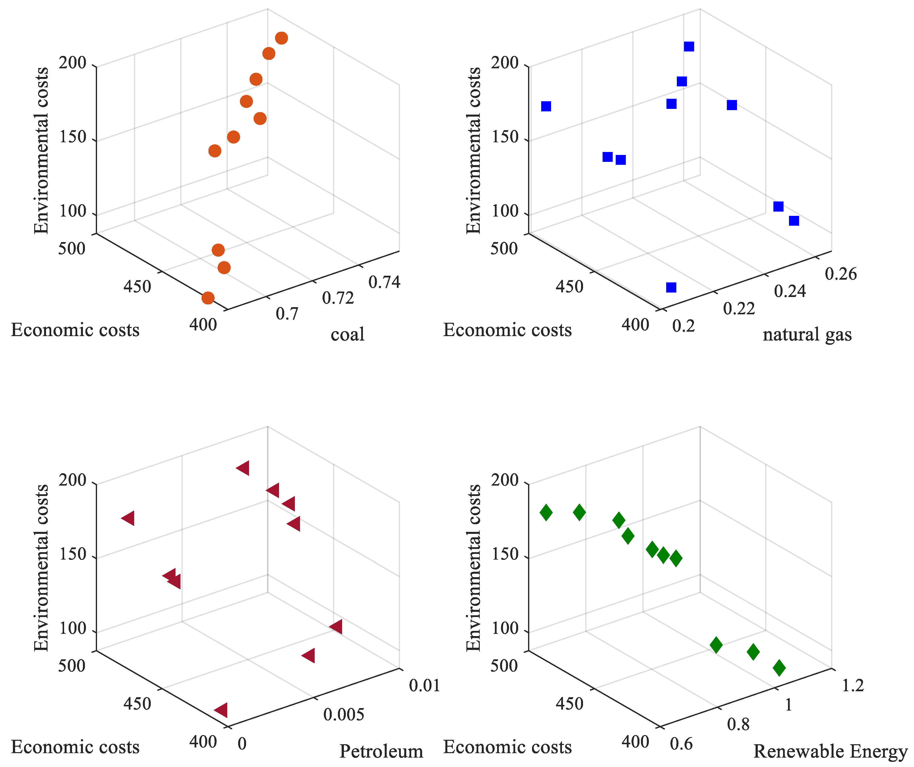
4.4.2. The Second Type of Planning Schemes

Under the second type of planning schemes, the urban energy system mainly uses natural gas and renewable energy as the main energy supply, and coal and petroleum are the auxiliary supply of energy, which are environment-friendly planning schemes. This planning scheme effectively reduces the pollutant emissions level, thus reducing the environmental cost. The feasible solution under the second type of planning scheme is shown in Figure 14. From the figure, we can see that although the total planned consumption of coal is less than that of the first type of planning scheme, its consumption is still positively correlated with the total target cost, indicating that the consumption and cost of energy, such as coal, have little correlation with the consumption of other energy. When the planned consumption of natural gas is less than 4000 tons of standard coal, with the increase of energy planning, the environmental cost has remained basically unchanged, while the total economic cost of energy is declining. It shows that in the second type of planning scheme, the relationship between natural gas planning volume and target cost is not sensitive. There are obvious fluctuations and faults in the relationship curve between the planned petroleum quantity and the target cost, indicating that in the second type of planning scheme, the planned petroleum consumption is the most sensitive factor to the target cost. In the change curve between renewable energy and target cost, due to the strong uncontrollability of renewable energy capacity, its large-scale use is greatly affected by other factors, and it is impossible to fit a strong correlation. However, it can be seen that the greater the consumption of renewable energy, the smaller the target cost.

4.4.3. Sub-Scenario Discussion

Since coal still plays an important role in the economy and society to ensure the security of energy supply and demand [34], this paper uses the growth rate of coal as the basis for scenario division, and adds the growth proportion constraint, based on the constraints proposed above, to bring into the second level of the planning model solution; each scenario is elected to find out the relationship between energy and cost under different development scenarios of urban energy planning.

• Scenario Ⅰ: 10% increase in coal planning

Simulation optimization is carried out under the constraint that coal consumption will increase by at least 10% in the future, and the top 10 feasible solutions are selected, which is shown as Figure 15. It is found that there is a relatively obvious linear relationship between the consumption of various energy sources and the total target cost. Among them, there is a positive correlation between coal and total target cost, while there is a negative correlation between other energy and total target cost. There is also a clear inflection point between petroleum, natural gas, and renewable energy, and the total target cost. The linear relationship between petroleum consumption and total target cost, and the linear relationship between renewable energy consumption and total target cost are more similar. When the petroleum consumption exceeds 8 tons, the economic and environmental costs decrease with the increase in consumption. When the consumption of renewable energy exceeds 8000 tons, the total cost decreases as consumption increases, and at a faster rate. However, when the consumption of natural gas exceeds 10,000 tons, the rate of decrease of the target cost with the consumption tends to be flat, indicating that when the planned natural gas consumption exceeds 10,000 tons, the consumption of natural gas is not a sensitive factor. Combined with the conclusions in the first type of planning scheme in the previous section, planners should pay attention to the inflection point of 10,000 tons. When the consumption of natural gas exceeds 10,000 tons, they should focus on controlling costs by changing the consumption of other energy sources.

2.

Scenario II: 10–20% reduction in coal planning

The simulation optimization is carried out under the constraint of reducing the coal consumption by 10% to 20% in the future, and the first 10 groups of feasible solutions are selected, which are shown as Figure 16. It can be found that both coal consumption and renewable energy consumption have a linear relationship with the total target cost. The total planning volume of coal is positively correlated with the total target cost, and the consumption of renewable energy is negatively correlated with the total target cost. As the consumption of renewable energy increases, there is a clear downward trend in total target costs. Comparing the two trend charts, it is found that under the same change trend of the total target cost, the total planned consumption of coal and the total planned quantity of renewable energy are negatively correlated. It shows that coal and renewable energy have a strong substitution relationship. When the planned coal volume is reduced, the energy steady-state can be maintained by increasing the consumption of renewable energy, and the total target cost can be reduced at the same time. When the consumption of natural gas is between 2400 tons of standard coal and 2600 tons of standard coal, the total planned amount of natural gas is positively related to the total target cost, but the fluctuation is small, indicating that the relationship between the planned amount of natural gas and the target cost is not sensitive. When the petroleum consumption is between 30 tons of standard coal and 80 tons of standard coal, the environmental cost and economic cost fluctuate greatly, indicating that the planned petroleum consumption is the most sensitive factor to the target cost in this situation. In this planning scenario, if planners want to further control the total target cost while using renewable energy to replace coal, they should give priority to controlling the consumption of petroleum.

3.

Scenario Ⅲ: 20% reduction in coal planning

The simulation optimization is carried out under the constraint of reducing coal consumption by more than 20% in the future, and the first 10 groups of feasible solutions are selected, which are shown as Figure 17. It can be clearly seen that only the consumption of coal maintains a relatively consistent linear relationship with the total target cost, with the total cost target essentially rising as coal consumption increases. However, the consumption of other energy sources cannot be fitted to the total cost target, which means there is no obvious linear relationship between the consumption of various energy sources and the total target cost. When the consumption of various types of energy in cities is different, the total cost has a certain degree of similarity. It shows that when the planned amount of coal is greatly reduced, the consumption of other kinds of energy is not stable, which will affect the stable state of an urban energy system, and the accurate total target cost cannot be obtained. If planners want to reduce the consumption of coal, they should appropriately reduce the consumption of coal according to the basic situation of an urban energy system, so as to avoid affecting the stability of the urban energy system by greatly reducing the consumption of coal.

4.4.4. Recommendation

With the development of urbanization, society pays extensive attention to environmental protection, the improvement of people’s living standards, the continuous improvement of the market economic system, and the social development and growth momentum of high-quality energy, such as natural gas and petroleum, which is gradually increasing. Under this energy development model, we should continue to strengthen the adjustment of industrial structure and optimize and upgrade the path of urban development. The focus is to strengthen the utilization of clean energy and improve energy efficiency, so as to further reduce the demand for traditional fossil energy in the process of economic development. Although the current coal-based system (in the first type of planning scheme) can still maintain a stable state, if the region chooses this development mode, it should try to adopt clean coal technology and coal to petroleum technology to make coal become clean energy. At the same time, since petroleum and natural gas are the most sensitive factor in the first type of planning scheme, when the consumption of natural gas is less than 10,000 tons, urban decision-makers should first consider adjusting the consumption of petroleum and natural gas when controlling the cost of energy consumption. Finally, when the urban development level of the region has reached a certain level, in the next step, the region must strive to reduce the proportion of coal in the energy consumption structure, and continuously reduce the proportion of direct coal consumption in the final energy consumption through industrial structure transformation and other measures.

Secondly, energy infrastructure plays an important role in urban construction and urban planning. From the experience of foreign urbanization development, the construction of an urban energy system is as important as the construction of road, transportation, communication, and drainage system. Urban energy system includes electricity, heat, gas pipe network, transmission and distribution system, and management system. The unified planning and construction of an urban energy system must appropriately promote urban development. While avoiding “urban disease”, it will further improve the level of urbanization and realize the sustainable development of cities and energy systems.

Third, the region must implement the strategy of “self production and self marketing of regional energy” and change the efficiency of energy production, transmission, and conversion. For example, through the implementation of CCHP, the heat energy related to thermal power generation can be directly supplied to users with the shortest streamline, which greatly improves the conversion efficiency of primary energy.

Finally, urban energy system planning is an important part of the top-level design of urban development, which is related to the sustainable development of the city. However, no matter what development model is adopted, the ultimate goal is to ensure the stability of urban economic development and reduce the emission of pollutants on the basis of meeting the energy demand. Smart city construction is not only the basis of scientific development, but also guides the optimal development of an urban energy structure. Through urban energy assessment and planning, the development of an urban energy system must be considered from the overall perspective of the city, then look forward to and carefully consider the city’s development strategy and development needs.

5. Conclusions

In order to realize the economic and environmental benefits of the urban energy system, a bi-level planning model for the steady optimal allocation of urban energy is established in this paper. The conclusions are as follows:

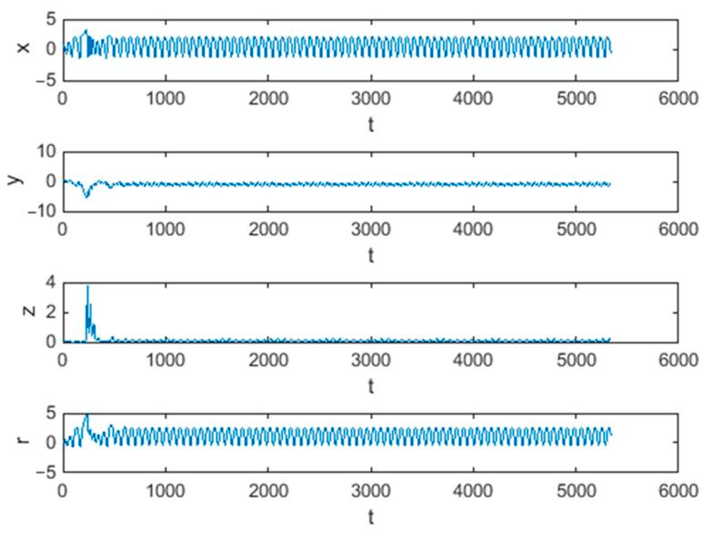
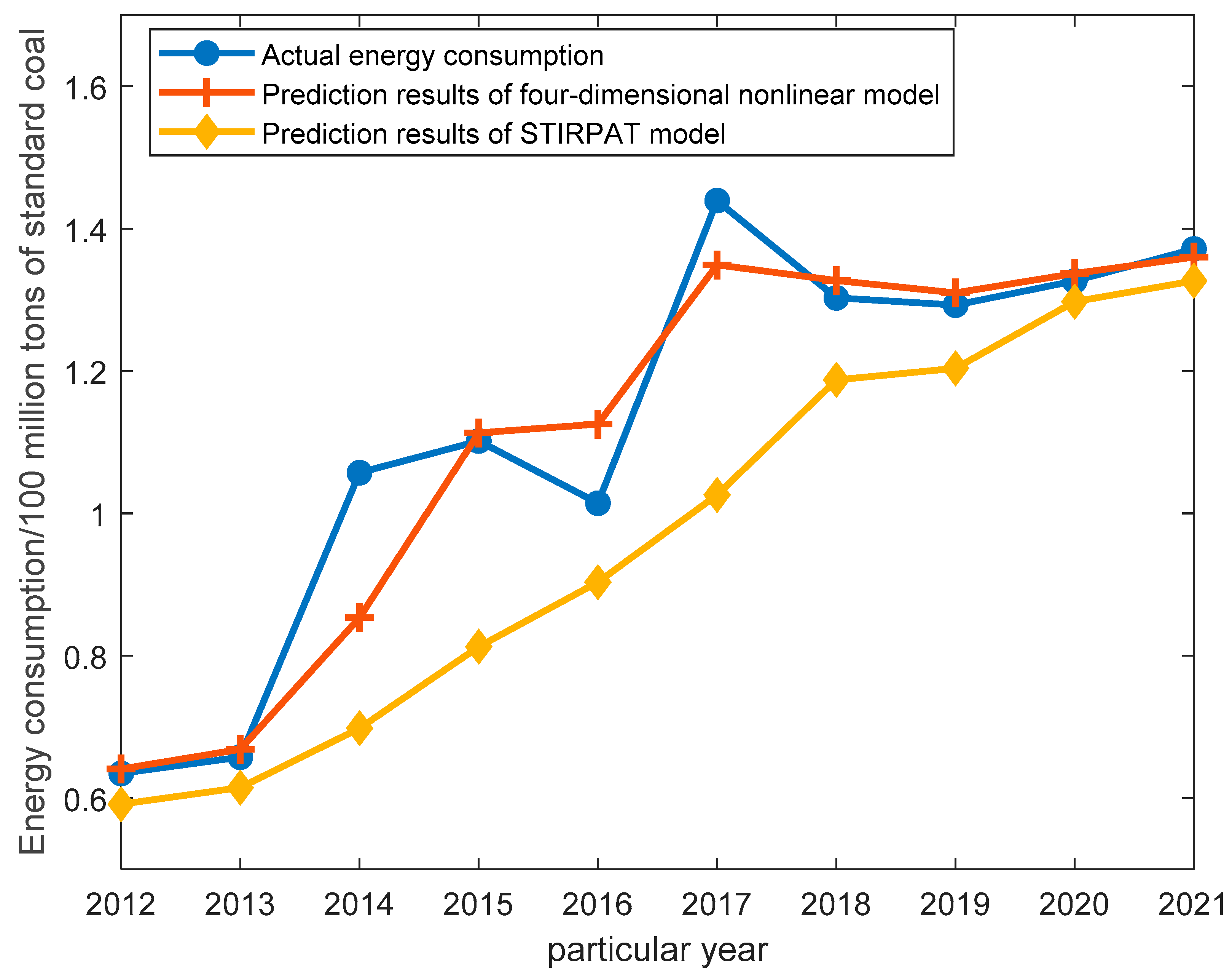
• In order to reduce energy consumption and optimize the urban energy structure, an urban energy steady-state model based on nonlinear system dynamics was developed on the basis of competing systems, and the relationship between coal, natural gas, petroleum, and renewable energy was studied. We used the consumption of coal, petroleum, natural gas, and renewable energy in certain region of China during 2005–2021 as the base data. It was found that the urban energy system could maintain a steady state when the parameters were as shown in Table 5. Compared with the method used in literature [24] to solve for the stability of urban energy systems, literature [24] considers more external factors related to energy usage (population size, affluence, etc.), while the method proposed in this paper is directly related to the endogenous factors of each type of energy (usage, elasticity coefficient, etc.), and the error with the actual data is 61.68% lower than that of literature [24].
• An optimization model for urban energy planning is proposed and solved using the IMFO algorithm. A comparison of the algorithms revealed that the improved algorithm in this paper finds the optimal solution faster than the original method, and that the feasible solutions are found to fall into two categories, coal-based and high- quality energy. The research found that in the coal-based scheme, petroleum and natural gas are the most sensitive factors related to the target cost. In the high-quality energy-based scheme, the relationship between the planned amount of natural gas and the target cost is not sensitive, and there is no strong correlation between renewable energy and target cost. Overall, without adding the constraint of coal energy consumption, where the smaller the share of coal is, the lower the cost.
• On the basis of the two-layer planning model for the optimal allocation of urban energy steady-state, the constraints of 10% increase, 10–20% reduction, and more than 20% reduction in the future planned coal volume were added, respectively, and the energy system of the region was carried out. In Scenario Ⅰ, we found that the results were basically consistent with the results of the coal-based scheme, but when the natural gas consumption exceeded 10,000 tons, the natural gas consumption was not a sensitive factor. In Scenario II, we found that coal had a strong substitution relationship with renewable energy. In Scenario Ⅲ, we found that only coal consumption maintained a relatively consistent linear relationship with the total target cost, however, the consumption of other energy sources could not fit a strong correlation with the total cost target. Through planning and simulation, it was found that the reduction of coal consumption should be carried out gradually (within 10%). If the coal consumption is suddenly reduced, the correlation between various energy sources and the target cost cannot be fitted, which will affect the urban energy stability to a certain extent.
• Although the above research results are presented in this paper, there are still some limitations. For example, in terms of modeling, the first-level model proposed in this paper is applicable to energy system stability prediction, and the solutions in this paper can actually find rigorous solutions mathematically, but there are also elements of trial, so the solutions obtained may only reflect part of the situation. However, they are still strictly analytical solutions and have their important theoretical value. At the same time, the second-level planning model can only solve planning usage problems for petroleum, coal, natural gas, and renewable energy, not practical operational problems. In terms of practical applications: this paper only examined the steady-state results and planning scenarios for urban energy systems. However, if planners want to achieve an optimal planning state for urban energy, city managers need to manage it through various macro-regulation means (e.g., giving clean energy subsidies through economic means, limiting coal consumption through policies, etc.), which requires follow-up research by scholars.

References

1. Webb, J.; Hawkey, D.; Tingey, M. Governing cities for sustainable energy: The UK case. Cities 2016, 54, 28–35. [Google Scholar] [CrossRef] [Green Version]
2. Teng, Z.Y.; Zhang, Y.; Li, X. Energy Internet—Integration of Information and Energy Infrastructure. Inf. Commun. 2018, 10, 265–266. [Google Scholar]
3. Mi, Z.F.; Guan, D.B.; Liu, Z.; Liu, J.R.; Vincent, V.; Neil, F.; Wang, Y.T. Cities: The core of climate change mitigation. J. Clean. Prod. 2019, 207, 582–589. [Google Scholar] [CrossRef]
4. Yu, S.H.; Sun, Y.; Niu, X.N.; Zhao, C.H. Energy internet system based on distributed renew able energy generation. Electr. Power Autom. Equip. 2010, 30, 104–108. [Google Scholar]
5. Grossman, G.M.; Krueger, A.B. Economic growth and the environment. Q. J. Econ. 1995, 110, 353–377. [Google Scholar] [CrossRef] [Green Version]
6. Ji, P.; Zhou, X.X.; Song, Y.T.; Ma, S.Y.; Li, B.Q. Review and prospect of regional renew able energy planning models. Power Syst. Technol. 2013, 37, 2071–2079. [Google Scholar]
7. Bo, P.; Xu, C.; Xu, Q.Y.; Zhang, N.; Kang, C.Q. Preliminary research on power grid planning method aiming at accommodating new energy. Power Syst. Technol. 2013, 37, 3386–3391. [Google Scholar]
8. Liang, H.; Long, W.D. Research and Application of Urban Energy System Comprehensive Planning Model. J. Shandong Jianzhu Univ. 2010, 25, 524–528 +557. [Google Scholar]
9. Yeo, I.A.; Yoon, S.H.; Yee, J.J. Development of an urban energy demand forecasting system to support environmentally friendly urban planning. Appl. Energy 2013, 110, 304–317. [Google Scholar] [CrossRef]
10. Yang, Y.F.; Han, L.; Wang, Y.R.; Wang, J.Z.; Jafari, N.N. China’s Energy Demand Forecasting Based on the Hybrid PSO-LSSVR Model. Wirel. Commun. Mob. Comput. 2022, 2022, 1–12. [Google Scholar] [CrossRef]
11. Xie, N.M.; Yuan, C.Q.; Yang, Y.J. Forecasting China’s energy demand and self-sufficiency rate by grey forecasting model and Markov model. Electr. Power Energy Syst. 2015, 66, 1–8. [Google Scholar] [CrossRef]
12. Filippov, S.P.; Malakhov, V.A.; Veselov, F.V. Long-Term Energy Demand Forecasting Based on a Systems Analysis. Therm. Eng. 2021, 68, 881–894. [Google Scholar] [CrossRef]
13. Wu, W.J.; Wu, J.K.; Lei, Z.; Zheng, M.J.; Zhang, Y.N.; Li, M.; Huang, X.; Li, Y.X. Energy demand prediction based on PSO Optimized BP neural network. Electr. Appl. 2021, 40, 49–58. [Google Scholar]
14. Zhang, Y.M. Research on China’s Energy Demand Forecasting Based on Combination Model. Master’s Thesis, Yan’an University, Yan’an, China, 2021. [Google Scholar]
15. Jing, R.; Kuriyan, K.; Lin, J.; Shah, N.; Zhao, Y.R. Quantifying the contribution of individual technologies in integrated urban energy systems—A system value approach. Appl. Energy 2020, 266, 1–15. [Google Scholar] [CrossRef]
16. Chen, C.; Su, M.R.; Yang, Z.F.; Liu, G.Y. Evaluation of the environmental impact of the urban energy lifecycle based on lifecycle assessment. Front. Earth Sci. 2014, 8, 123–130. [Google Scholar] [CrossRef]
17. Kagaya, S.; Ueda, M. An Evaluation on Improvement of the Urban Energy System in a Snowy Cold Region. Environ. Syst. Res. 2010, 23, 204–213. [Google Scholar] [CrossRef] [Green Version]
18. Xie, S.; Jia, Y.L.; Bai, X.T.; Zhang, Z.H.; Wang, S.Y.; Zheng, X.Y.; Zhao, Y.R. A review of urban energy system planning and design and energy consumption analysis tools. Glob. Energy Internet 2021, 4, 163–177. [Google Scholar]
19. Zheng, X.Y.; Qiu, Y.W.; Zhan, X.Y.; Zhu, X.Y.; Keirstead, J.; Shah, N.; Zhao, Y.R. Optimization based planning of urban energy systems: Retrofitting a Chinese industrial park as a case-study. Energy 2017, 139, 31–41. [Google Scholar] [CrossRef]
20. Neshat, N.; Hadian, H.; Alangi, S.R. Technological learning modelling towards sustainable energy planning. J. Eng. Des. Technol. 2020, 18, 84–101. [Google Scholar] [CrossRef]
21. Yazdanie, M.; Orehounig, K. Advancing urban energy system planning and modeling approaches: Gaps and solutions in perspective. Renew. Sustain. Energy Rev. 2021, 137, 110607. [Google Scholar] [CrossRef]
22. Su, M.R.; Chen, C.; Yang, Z.F. Urban energy structure optimization at the sector scale: Considering environmental impact based on life cycle assessment. J. Clean. Prod. 2016, 112, 1464–1474. [Google Scholar] [CrossRef]
23. Wang, R.X.; Li, H.; Xing, M.B.; Xue, R.J. An approach to urban energy planning from the perspective of all-energy flow. Sci. Technol. Eng. 2019, 19, 365–370. [Google Scholar]
24. Shen, M.; Shen, L.; Zhang, Y.; Liu, L.T.; Xue, J.J.; Chen, F.N. Analysis on stability and influencing factors of energy supply system in Shaanxi Province. Econ. Geogr. 2015, 35, 39–46. [Google Scholar]
25. Li, A.M.; Zheng, H.M. Energy security and sustainable design of urban systems based on eco-logical network analysis. Ecol. Indic. 2021, 129, 1–10. [Google Scholar] [CrossRef]
26. Zhu, X.T.; Mu, X.Z.; Hu, G.W. Ecological network analysis of urban energy metabolic system—A case study of Beijing. Ecol. Model. 2019, 404, 36–45. [Google Scholar] [CrossRef]
27. Kazaoka, R. Nonlinear dynamics and stability of an electric power system with multiple homes. Ieice Tech. Rep. Non-Linear Probl. 2011, 111, 67–72. [Google Scholar]
28. Zhao, H.S.; Xue, N.; Shi, N. Nonlinear Dynamic Power System Model Reduction Analysis Using Balanced Empirical Gramian. Appl. Mech. Mater. 2013, 448–453, 2368–2374. [Google Scholar] [CrossRef]
29. Du, T.; Zeng, G.H.; Huang, B.; Wei, Y. PMSM vector control optimization based on improved moth-to-fire optimization algorithm. Sens. Microsyst. 2021, 40, 52–55. [Google Scholar]
30. Long, W.; Jiao, J.J.; Zhang, W.Z.; Xu, M.; Cai, S.H. An Improved Moth Flame Optimization Algorithm for Solving High-Dimensional Global Optimization Problems. Pract. Underst. Math. 2020, 50, 153–163. [Google Scholar]
31. Zhao, Q.; Mao, Q.H.; Liang, P. Research on location selection of electric vehicle charging station based on improved moth algorithm. J. Hunan Univ. Arts Sci. 2021, 33, 12–19. [Google Scholar]
32. Qin, T.; Xiang, T.M.; Li, B.B. Optimization of Microstrip Antenna Design Based on Improved Moth to Fire Algorithm. J. Hangzhou Dianzi Univ. 2020, 40, 13–18. [Google Scholar]
33. Ministry of Ecology and Environment of the People’s Republic of China. Measures for the Administration of Emission Fee Collection Standards. 2003. Available online: https://www.mee.gov.cn/ywgz/fgbz/gz/200302/t20030228_86250.shtml (accessed on 1 March 2022).
34. Liu, F.; Guo, L.F.; Zhao, L.Z. Coal safety zone and green low-carbon technology path under the background of double carbon. J. Coal 2022, 47, 1–15. [Google Scholar]
Figure 1. The relationship between urban energy structure and urban sustainable development.
Sustainability 14 06485 g001
Figure 2. Typical structure of an Urban Energy System.
Sustainability 14 06485 g002
Figure 3. Structure of the bi-level optimization.
Sustainability 14 06485 g003
Figure 5. Energy consumption of the region in China in 2005–2021.
Sustainability 14 06485 g005
Figure 6. Three-dimensional view of the city energy system.
Sustainability 14 06485 g006
Figure 7. d 3 = 0.13 and time series of x ( t ) , y ( t ) , z ( t ) , r ( t ) .
Sustainability 14 06485 g007
Figure 8. Comparison of projected energy consumption results.
Sustainability 14 06485 g008
Figure 9. Algorithm comparison chart about Economic Cost (a) and Environment Cost (b).
Sustainability 14 06485 g009
Figure 10. Pareto results of economic goals and environmental objectives.
Sustainability 14 06485 g010
Figure 11. Energy structure and cost structure of different planning solutions.
Sustainability 14 06485 g011
Figure 12. Two planning schemes: mainly coal or high-quality energy.
Sustainability 14 06485 g012
Figure 13. The first type of planning schemes: based on coal.
Sustainability 14 06485 g013
Figure 14. The second type of planning schemes: based on high-quality energy.
Sustainability 14 06485 g014
Figure 15. Planning scenario for a 10% increase in coal.
Sustainability 14 06485 g015
Figure 16. Planning scenarios for a 10–20% reduction in coal.
Sustainability 14 06485 g016
Figure 17. Planning scenarios for a 20% reduction in coal.
Sustainability 14 06485 g017