
An Inter-Temporal Computable General Equilibrium Model for Fisheries
by
 , , and
Haoran Pan
1,2,*, 
Pierre Failler
3 ,
,
Qianyi Du
1,2,
Christos Floros
4,
Loretta Malvarosa
5,
Emmanuel Chassot
6 and
Vincenzo Placenti
7 1
School of Economics and Resource Management, Beijing Normal University, Beijing 100875, China
2
Center for Innovation and Development Studies, Beijing Normal University, Zhuhai 519087, China
3
Centre for Blue Governance, Faculty of Economics and Law, University of Portsmouth, Portsmouth PO1 3LJ, UK
4
Department of Accounting and Finance, Hellenic Mediterranean University, 71410 Heraklion, Greece
5
NISEA, Fishery and Aquaculture Economic Research, 84100 Salerno, Italy
6
Institut Agro, Fisheries and Aquatic Sciences Center, 35 042 Rennes, France
7
ARGO Srl, 84064 Salerno, Italy
*
Author to whom correspondence should be addressed.
Sustainability 2022, 14(11), 6444; https://doi.org/10.3390/su14116444
Submission received: 14 April 2022
/
Revised: 11 May 2022
/
Accepted: 13 May 2022
/
Published: 25 May 2022
(This article belongs to the Special Issue Integrated Modelling for Sustainable Fisheries Management)
Abstract
:Computable general equilibrium models have been a popular tool for policy analysis in recent decades, but rarely applied for fisheries policy and management. This paper presents an inter-temporal computable general equilibrium model with fisheries details. While the model in a full-scale and disaggregate way describes the structure and dynamics of a regional fisheries economy, it further specifies the heterogeneous bottom-up fish producers, such as harvesters, aquaculture and fish-processing firms, and links fisheries with the top–down non-fisheries economic sectors. In addition, the model can be externally linked with fish biological models to consider interactions between economic and biological systems. The model is designed to provide a comprehensive tool for analysis of new fisheries policy in general and to study five European fishery regions in particular. The empirics in the paper evaluate the impact of several important management and policy instruments on the Salerno economy and on recovery of endangered species.
JEL Classifications:
C68; O13; Q22; Q56; Q571. Introduction
Marine fisheries management is an effective and important tool to ensure the sustainable development of the ocean. Fisheries management aims to establish a more effective balance at ecological, economic and social levels [1]. To study fisheries sustainability, current researchers will consider more the impact of new fishery policies on ecology, society and economy simultaneously [2], and then put forward comprehensive suggestions for current fishery policies, instead of a single-dimensional assessment. Fisheries planning and management require environmental, social and economic assessments that take into account multiple sustainability criteria and the preferences and priorities of decision-makers involved in fisheries planning [3]. As global fisheries management shifts to ecosystem-based management, policymakers need to assess the potential impact of this shift on fishermen and the economy [4]. In sustainable fisheries resource management, a better understanding of the interaction between complex ecological processes and socio-economic systems is required in order to comprehensively and accurately assess the possible impact of fisheries policies [5]. Through computable general equilibrium (CGE) modelling, many fisheries-related management and policy issues can be addressed. In this research we develop a standard, SAM-based, multi-sector, multi-agent, inter-temporal dynamic CGE model with fisheries details. The full economic structure of the model allows analysis of the economy-wide interrelating effect between fisheries and the rest of the economy. The particular forward-looking feature of the model is consistent with a fisheries management and policy regime where current decisions will affect the future price and stock of aquatic products, which, in turn, will impact on the current decision making.
For the economies where fisheries are the mainstay of the economy, computable general equilibrium models have non-negligible advantages. For countries or regions with a high share of fisheries GDP, if the study only uses the partial equilibrium models, the research subjects are limited to the fisheries sectors, which cannot measure the impact of fisheries policies on the macroeconomy.
Our study makes new contributions to the general equilibrium model of fisheries.
- A multi-sector, multi-agent, inter-temporal dynamic CGE model is developed. “Inter-temporal dynamic” means that given the final expected policy objective throughout the decision period, the model is solved for the optimal decision in each period simultaneously. Moreover, it can facilitate managers to consider long-term decision making. “Multi-agent” in this paper splits the households into fishing households and non-fishing households so that it can be used to focus on the labor market of fishing households. “Multi-sector” in this paper divides the fishery sectors into fishing, aquaculture and fish-processing sectors, and it distinguishes the difference between different fishing activities.
- The ecosystem is connected to the economic system and can capture the dynamic interactions between the systems. On the one hand, fishing activities affect the biomass stock and influence the ecological sustainability of fisheries; on the other hand, fishing activities also determine fishers’ income and macroeconomic conditions. Integrating marine fisheries ecosystems with economic systems can provide more comprehensive policy insights for government fisheries managers.
The aim of this study is to provide a new comprehensive model that can evaluate and optimize fisheries policy and management in countries or regions where fisheries are the backbone of the national economy. This study provides a scientifically quantifiable and integrated tool for governments and agencies to analyze fisheries policy management and to help them better understand the interactions between complex ecological processes and socio-economic systems. It helps to integrate ecosystems and economic systems to consider policy implications. The most important contribution of our research is to develop a new approach for fisheries policy and management and to present the innovative points of the approach in this paper. We do not focus on presenting how to solve a specific fisheries policy problem that exists in Italy. Instead, our empirical analysis section provides examples of model application, including policy scenario settings and analysis of results, confirming that the model can be applied to fisheries policy management. Using the proposed model, we examine the effectiveness of some management or policy instruments, such as consumption tax on the fish, production tax on the harvesting of the fish and total allowed catch (TAC), in combination with capacity withdraw, as per the Salerno economy case. Other research scholars can further apply this model to solve more specific fishery problems in practice.
In addition, the replicability of the model lies in the fact that the model can also be applied to other developed or developing countries or regions where fishing is the mainstay of the economy, or to islands, and thus not only to the Italian Salerno economy, which has the following characteristics: firstly, marine fishing is the mainstay of the economy, and the chain of industries related to fishing is longer; secondly, this is a region of traditional fishing, close to the sea, where the inhabitants depended on fishing for their livelihood throughout history. This model can be used whenever the interaction between the economic and marine fishery systems needs to be considered. This model belongs to the frontier of fisheries economics models, a general equilibrium model with inter-period dynamics. However, this model does not apply to the analysis of non-fishing countries or regions where the contribution of fisheries to the economy is negligible. The present paper is organized as follows. Section 2 presents the literature review. Section 3 describes the general structure and innovative design of the model. Section 4 applies the model to the Salerno economy in Italy, to illustrate how it can be used to study fishery-related issues. Finally, we conclude the work and provide policy implications in Section 5 and Section 6.
2. Literature Review
Contemporary fisheries economics have been dominated by partial equilibrium analysis of capture fisheries, with primary interest in the static bionomic [6,7] and dynamic bioeconomic [8,9,10] relationships between harvesting, biomass stock and growth of one or two commercially important species. Some literature focuses only on the growth patterns of ecosystem fish populations, focusing on optimizing methods to make more accurate predictions of fish populations, but not on the impact of their changes on the economic system [11,12]. Van Dijk et al. (2014) considered the behavioral interactions between policymakers and fishers that combine to affect fish stocks and capital stocks, but the model still lacked links to the economic system [13].
While partial equilibrium analysis allows clear focus on particular fishery issues, it ignores the interactions between capture and non-capture fisheries, and between fisheries and non-fisheries economic sectors; it also misses consumer markets where aquatic demands, substitutability between aquatic products, substitutability between aquatic and agricultural products, and welfare analysis should have influence on fisheries policy. Therefore, many scholars have tried to consider policy directions from fisheries management policies by combining ecological and economic implications in recent years, but there are some shortcomings. Tokunaga et al. (2019) used the Catch-MSY model when studying Japanese fisheries and then input the model’s results into the Pella–Tomlinson model to consider some economic variables, such as profits. However, this method does not integrate ecosystems and economic systems, and it cannot study the endogenous interactions between the two systems [14]. Rosa et al. (2022) attempted to develop a bioeconomic model that considers more economic factors to define controlled fishing rules, which could enhance policy design aimed at coordinating economic returns to fisheries and stock recovery. Nevertheless, this is not a general equilibrium model and does not capture the interaction between ecological and economic systems [15].
Another unforgivable missing aspect in fisheries economics is the price mechanism, which is often fixed or exogenously projected to the future during analysis. Furthermore, the primary focus of fisheries economics on microeconomic behaviour causes a gap in the macroeconomic analysis related to fisheries, such as international trade, labor substitution and migration, industrial transformation, regional economic growth, etc. However, this problem can be solved by using a computable general equilibrium model.
Only few researchers have conducted general equilibrium analysis for the fisheries industry, while most of them are stylized rather than applied analysis. Seung and Waters [16] reviewed unpublished research that has built up an applied general equilibrium model for Oregon’s regional fisheries. The study specified five fishing sectors, five fish-processing sectors and 24 other sectors, including three types of factor incomes, household income categories, two government expenditures, imports and exports, and investment. According to the review, it sounds as if the Oregon model is a static CGE model, which cannot be appropriately tied to marine biological process; therefore, the impact of fishing activity on marine systems is not assessed, and the feedback from marine systems to economic systems is exogenously given. In other words, the model does not specify endogenous interactions between the fisheries and fish stock changes.
While some scholars have used computable general equilibrium models to study the fishing economy, there is no further detailed splitting of fishing sectors and households. The lack of long-term decision-making considerations (dynamic mechanism) may limit the policy implications. Waters and Seung (2011) used a computable general equilibrium (CGE) model to study the effects of harvest reductions on Alaskan fisheries, which contained 18 industries. However, only four industries were fish-related and primarily considered Pollock as a fish species [17]. Carvalho et al. (2011) used a recursive dynamic CGE model to study the impact of the elimination of fisheries subsidies on the small island economy of the Azores, which uses a dynamic mechanism but is also a recursive dynamic, not intertemporal dynamic [18]. The intertemporal dynamic can solve the decision solution for all years given the expected target, which obviously cannot be achieved in this model. There are 45 sectors in the model, of which only one is the fisheries sector, so it is not built explicitly for the fisheries sector and has a less detailed fisheries part. Jin et al. (2012) relates a computable general equilibrium (CGE) model of the coastal economy to the Georges Bank end-to-end (E2E) model of the marine food web. Although it can consider both marine animal impacts and consumer income effects, it takes more of a submarine food chain perspective. Then the consideration is static, not intertemporal dynamic, so it is hard to make decisions every year simultaneously [19]. Da-Rocha et al. (2017) used data from different fleets producing different fishes [20]. The framework for fisheries details is not well designed. Moreover, they assume that a typical household owns a fishery plant, which means there is no splitting of the household sector. In our model, fisheries details are set up with a more detailed production nested structure, including harvesting, aquaculture, and fish processing firms. Moreover, it is a bottom-up model and subdivides the harvesting firms into different fleets that can produce different types of fish. We split the standard households into fishing and non-fishing households, which is an important distinction from other papers that will have more policy implications in policy simulations, such as distinguishing changes in income and welfare of different types of households. There is another group of fisheries economic models that simulate both economic and ecological systems and integrate them together, using general equilibrium theory [21,22,23]. They believe the ecosystem follows the general equilibrium theory and prices drive species to compete for survival. While it is highly arguable in science whether the general equilibrium theory can be adequately applied to the ecosystem, those models only specify a small or simplified, dynamic, optimizing economic component but concentrate on dynamic interactions of species in ecosystem. They may possess some general equilibrium features but are different from the standard, SAM-based, multi-sector general equilibrium models, and thus limited in providing economic insights.
There is also some literature that use input–output analysis, social accounting matrix and other methods to capture the effects of fishery management policies, their disadvantage is linearity. Kaplan and Leonard [24] combined the fishery ecosystem model with the economic model (IO-PAC) to explore the potential impact of a wide range of fishery management options. Santiago et al. [25] utilized a new model developed in the input–output framework to assess the socio-economic impact related to the determination of annual fishing quotas by species in the main fleet segments managed by the EU. Kim and Seung [26] established a social accounting matrix (SAM) model to study the distributional effects and economic contribution of two different fish-producing industries in Gyeong-Nam Province, Korea. However, the models mentioned above are mainly linear. Although linear economic models can measure the ecological and economic effects of fishery policy, compared with the computable general equilibrium model, there is a disadvantage that the price is fixed in the linear system, meaning the substitution between goods and services is not allowed [27]. The computable general equilibrium model can not only be used to evaluate the ecological and economic effects of fishery policies on multiple sectors, but also have the function to substitute the goods and services according to the relative price. The models are strictly based on microeconomic theories such as maximizing producer profits and maximizing consumer utility.
The most significant contribution of our CGE model is that it links both the economy and the ecosystem into one system and establishes the interaction between the two. The second thing is that our model is multi-sectoral and multi-agent. Moreover, our model has more details about fisheries industries. In addition, our model includes the dynamic mechanism, which is an inter-temporal dynamic rather than a recursive dynamic. The inter-temporal dynamic mechanism allows us to stand on the whole picture to make decisions in each period. Our model is designed to serve countries or regions where fisheries are the central economic pillar. Using general equilibrium theory, the model ensures that fisheries interact with other industries to reflect the macro level, thus providing more comprehensive information for policymakers’ policy evaluation, i.e., more ecological and economic indicators.
3. The Structure of the Model
The present model is a disaggregated, inter-temporal, dynamic general equilibrium model. Its construction basically follows standard routines of computable general equilibrium (CGE) modelling, as described in the literature [7,28,29], but gives special treatment to fisheries. Because of its large scale, it is inappropriate to present the full model in this paper. Instead, we focus on some key equations regarding optimizations for consumers and producers, with a particular focus on fisheries.
3.1. Consumer Behaviour
This research is of particular interest in the fishery policy and fishery society; thus, the model is set up to consist of two types of representative consumers, namely, the general non-fisheries households and fisheries households. The latter depends on the fisheries income, including not only capture fisheries, but also aquaculture and fish-processing, while the former depends on the income not related with fisheries. This classification enables policy analysis to assess the welfare change of the fisheries society.
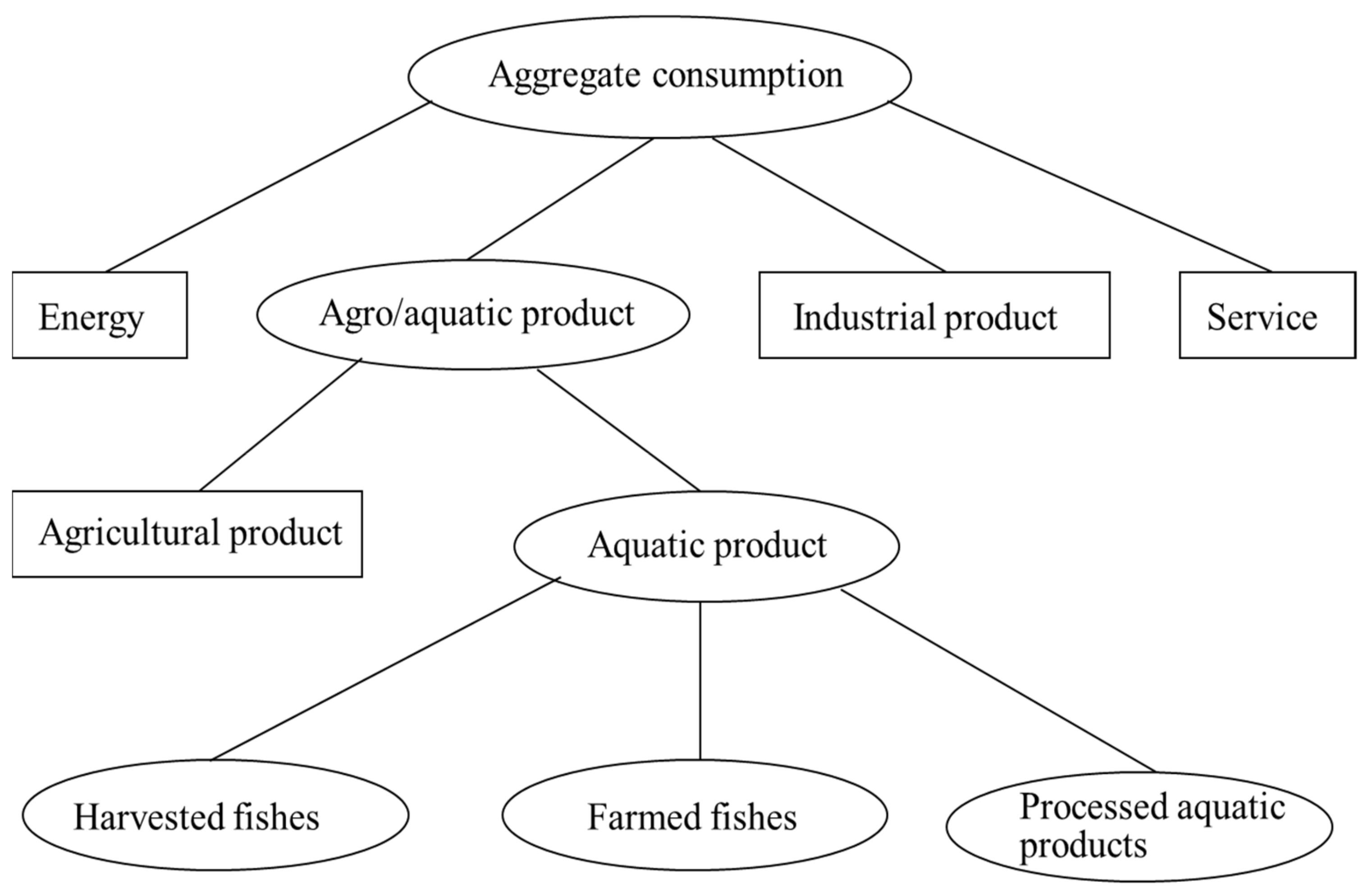
Household consumption is defined according to a multi-level nested system (Figure 1).
At the top level, a representative household maximizes her inter-temporal utility across entire time periods by optimally allocating aggregate consumption over the time (the Ramsey rule) subject to inter-temporal budget constraints. The representative consumer’s objective is
where is the social or pure time preference or discount rate and is the aggregate consumption in volume at time . The utility function is the logarithm of the aggregate consumption. The time duration has periods. Subject to:
where is total expenditure during the periods, is the real interest rate, and are the price of aggregate consumption and the income at time , and and are the exogenous initial and end period savings, respectively. The left-hand side of the above equation is the consumer’s total spending and the right-hand side the total income during that period.
The first-order conditions together with the budget constraint give the following solution system for consumption variables :
Obviously, the consumption demand depends on both the consumption price and income level, which are determined by the price system and factor income distribution.
Once the aggregate consumption is set up in each period, it is divided into four consumption or commodity categories, namely, composite agricultural and aquatic product (aa), energy (eng), industrial product (ind) and services (sev). The demands for these products are derived from minimizing the Stone–Geary expenditure function at a given level of utility in a specific period. Assuming that each of the consumption or commodity categories also include a minimum obliged consumption as a part, and that the budget share of expenditure on each category is fixed and all shares add up to one, we adopt the Stone–Geary utility function to define the following total expenditure function in period :
where is total expenditure for the second level of consumption at period , is commodity i’s price of the disaggregate consumption, is the minimum obliged or subsistence consumption of commodity and the marginal budget share of consumption of commodity . Minimizing the above expenditure function, we obtain the Hicksian-derived demand function with respect to each commodity.
The above equation says that the Hicksian-derived demand for a commodity depends on relative prices, aggregate consumption and shares. The minimum obliged consumption can be either exogenously given or endogenously determined according to defined relationships with relative prices, aggregate consumption, budget shares and expenditure elasticity.
Among the four commodities at the second level of consumption, energy, industrial product and services are the final products produced by the respective sectors, while composite agricultural and aquatic products are hypothetical products that need to be disaggregated further into agricultural and aquatic products at the third level of consumption. Such a design allows for greater substitution between the two products. Here, we assume the CES utility function with the following expenditure function:
where is the total expenditure for agricultural and aquatic products, and and are the price and consumption of the composite agricultural and aquatic products, respectively. is the substitution elasticity at the third level of consumption, and and are the share parameters of the agricultural and aquatic price, respectively. Minimizing the above expenditure function, we obtain the Hicksian-derived demand function with respect to each of agricultural and aquatic products.
where agricultural product, , is the final product of the agricultural sector, but aquatic product, , is a composite product of the aquatic sector, which needs to be disaggregated further into various aquatic products. This moves us to the fourth level of consumption. We again assume the CES utility function and have the following expenditure function:
where is the total expenditure for fish or aquatic products; , and represent harvested fish, farmed fish and aquatic products, respectively; is the substitution elasticity at the fourth level of consumption; and are the share parameters of fish species or aquatic products. Minimizing the above expenditure function, we obtain the Hicksian-derived demand function with respect to each of the fish or aquatic products.
The demands obtained at this level are the final products of the fish harvesting, aquaculture and fish-processing sectors, by species. For simplicity, we do not model marketed and home-consumed aqua-products here. Instead, we assume that all aqua-products are marketed. In future research, one may either assume that fixed proportions of the total aqua-products are marketed or follow the above example to model the substitution between the marketed and home-consumed aqua-products.
3.2. Producer Behaviour
This model contains a mix of top–down general economic sectors and bottom–up fisheries producers in order to study fisheries in great details. The top–down sectors are simply aggregated non-fisheries sectors, including agriculture, energy, industry and services. Modern fishing activity relies heavily on fossil fuels, the emissions of which are believed responsible for climate change. Thus, the separate consideration of the energy sector would provide convenience for study of the interrelations between fisheries and climate change policies. Agriculture has the closest link with fisheries, not only because agricultural and aquatic products are highly substitutable, but also because production factors, particularly labor, are highly mobile between the two sectors. Industry and services are the largest two sectors in most economies. They provide products and services to the fisheries. Since this research focuses on fisheries product, we simply assume that each of the top–down sectors produce a single product only. For example, the industrial sector produces industrial products.
The bottom–up fisheries producers include harvesting, aquaculture and fish-processing firms. There are other types of firms, such as fish marketing, recreational fisheries and fishery-business service firms, that are related to fisheries but normally embodied in the service sector. Because those firms cannot be accurately identified by normal data collection, we do not consider them separately in this research. The harvesting producer is broken down into a number of métiers (the bottom–up fish producers), which is defined as a particular fleet equipped with a particular gear, targeting a particular species and having by-catch. Thus, each métier may produce multiple products. Aquaculture can be considered to consist of various types of farms, each of which specializes in farming a single species. As a whole, aquaculture is regarded to produce multiple farmed species or products. Similarly, fish-processing firms are also grouped into different types by the final product they produce. For example, a processing firm may specialize in processing the salmon by a number of processing methods. In this way, the top–down structure of the model is connected to the bottom–up specification of fish production.
3.2.1. The Top–Down Non-Fisheries Producers
The production of the top–down non-fisheries producers follows a multi-level nested system (Figure 2) in which producers maximize the net present value of revenue across time by optimally allocating investment across all time periods and employing intermediate and factor inputs for production activity within each time period. The producers are assumed to use a four-level nested CES technology, allowing different rates of substitution among composite intermediate products and factors, among general products, and among species and aquatic products.
At the top level, each top–down producer uses a composite intermediate product and factor to produce a single output and maximizes its inter-temporal profit for a particular duration of time subject to inter-temporal constraint of the capital accumulation. The solution of the problem will determine the trajectory of optimal investment across time and the demands for various intermediate and factor inputs in each period.
where ir is the real long-term interest rate, and ,, and are the general producer ’s output, composite intermediate input bundle, composite factor input and investment, respectively. , , and are the corresponding prices and , , and represent agriculture, energy, industry and service, respectively. For convenience, we omit the subscript for all input terms.
Subject to:
where is producer ’s capital stock at time , is the depreciation rate of the capital and the exogenous initial capital stock. Assuming aggregate production in each period takes the CES technology, we have
where and are the share parameters of and . is the elasticity of substitution between and in the non-fisheries sectors. This dynamic optimization problem can be conveniently solved with the Bellman recursive method for the following solutions:
Demand for composite intermediate product,
Demand for composite factor,
Supply of capital,
and Demand for investment,
At the second level, the intermediate product is the CES function of a composite agricultural and aquatic product (aa) and a composite product of energy, industrial product and service (eis). The substitutability between them is assumed to be low. Given the total demand for aggregate intermediate products, minimizing the production cost, we have
where and are demands for aa and eis, respectively. and are their prices. Subject to:
where and are the parameters adjusted to the base year data. is the elasticity of substitution between and . The solutions of this problem are as follows:
Demand for composite aa and eis products are
where by duality.
At the same level, the composite factor is the CES function of capital and labor. Given the total demand for composite factor, minimizing the factor cost, we have:
where and are demands for capital and labor, respectively. and are rental and wage rate, respectively. Subject to:
where and are parameters adjusted to the base year data. is the elasticity of substitution between capital and labor. The solutions of this problem are as follows:
Demand for capital and labor are
where by duality.
Further down to the third level of production, both composite products are disaggregated into aquatic, agricultural, energy, industrial, and service product, respectively. Given and , cost minimization solves for the optimal demands:
where and are demands for agricultural and aquatic products, respectively. and are their prices. Subject to:
where and are parameters adjusted to the base year data. is the elasticity of substitution between and . The conditional demand functions of this problem are:
Similar for , the conditional demands are
where are parameters adjusted to the base year data; and are demands and prices for energy, industrial product and service, respectively; and is the elasticity of substitution between the energy, industrial product and service.
At the bottom level of the production, given the total demand for composite aquatic product, cost minimization solves the production demands for species or aquatic products. The conditional demand functions of this problem are
where are parameters adjusted to the base year data; and are demands and prices for different species of fishes, respectively; is the elasticity of substitution between inputs of fish; and, , and represent harvested, farmed and processed species or aquatic products, respectively.
3.2.2. The Bottom–Up Fisheries Producers
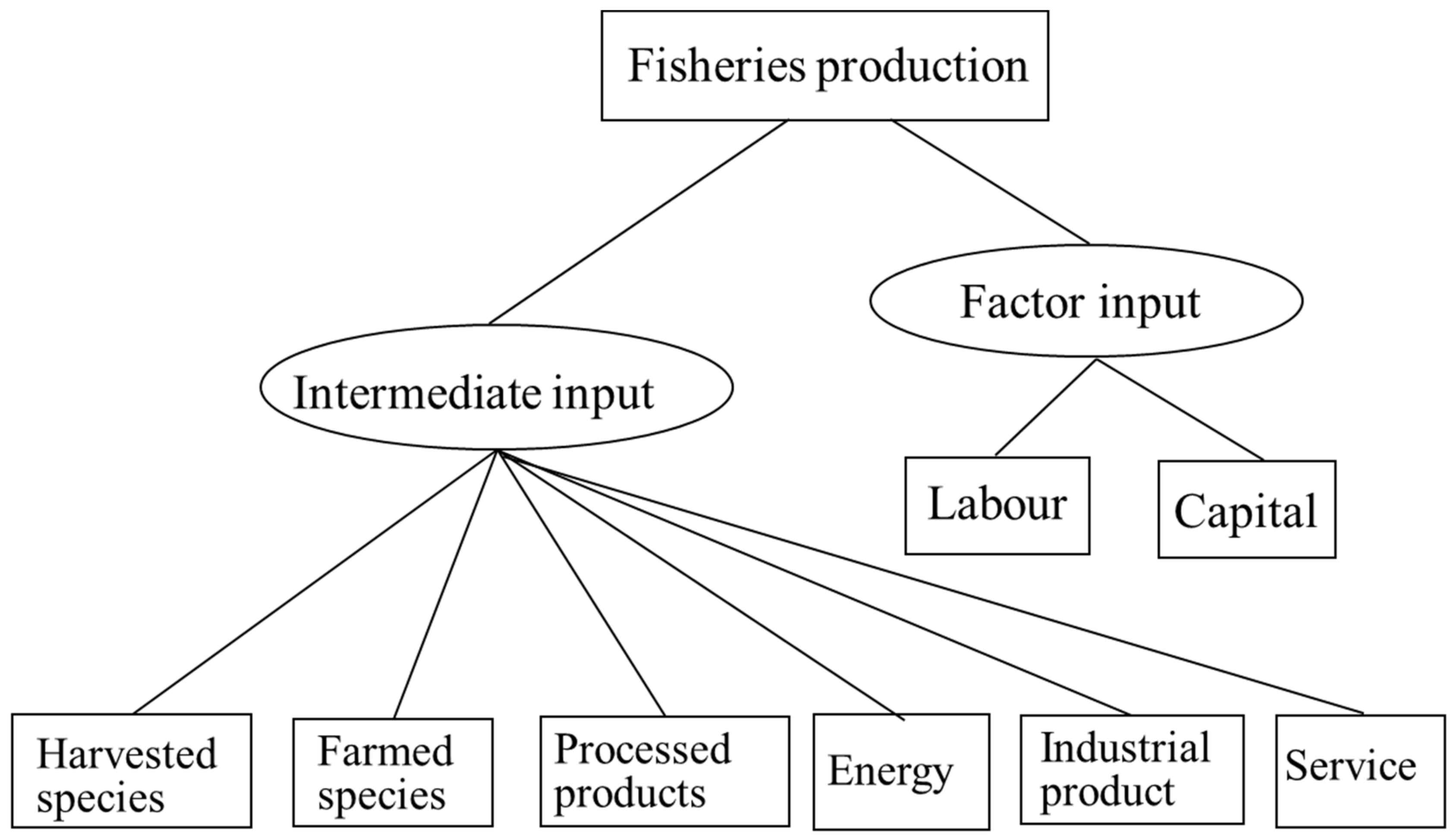
The fish harvesters, aquaculture and fish-processing producers are the bottom–up fish producers, which are assumed to produce with a two-level nested technology (Figure 3). At the top level, they are similar to the non-fisheries producers in that they use composite intermediate product and factor with CES technology to produce outputs. At the second level, the fisheries producers have a more simple production structure than the non-fisheries in that they disaggregate composite intermediate input by the Leontief technology, where intermediate inputs are assumed to be used in fixed proportion, and the disaggregate composite factor with CES technology into capital and labor. In fisheries economics, the harvesting sector pays workers by a proportion of total catch or by fishing effort rather than by wage rate. For the sake of merging the harvesting sector with other sectors our model, the model adopts the standard economic approach of labor and capital inputs. While the aquaculture and fish-processing producers are regarded to consist of a number of different producers, each of which represent a group of identical individual producers and specializes in a single species of fish, the fish harvesters consist of a number of métiers, each of which may harvest multiple species.
Fish harvesting involves not only physical capital stock but also biomass stock. Unlike physical capital, biomass is a common property that can be available to any harvesters. Therefore, individual harvesters cannot manage the biomass stock, which sounds like a common pool property and does not enter into their fishing decision. In this sense, the harvesters behave in a way similar to other producers by maximizing profit subject to dynamic accumulation of physical capital. This approach differs from the approach of dynamic optimal control in conventional fisheries economics where either biomass stock or both biomass and physical stocks are state variables [8,10,30].
At the top level the fisheries producers maximize their inter-temporal profit for a particular duration of time subject to inter-temporal constraints of capital accumulation
Subject to:
Assuming aggregate production of each producer in each period takes the CES technology, we have
where is the elasticity of substitution between and in the fisheries sectors. The solutions of the problem are:
Demand for composite intermediate product,
Demand for composite factor,
Supply of capital,
and Demand for investment,
At the second level, the composite intermediate product is disaggregated by the Leontief technology:
where are the fixed proportion of intermediate inputs and intermediate demands.
At the same level, the composite factor is disaggregated in a similar way to the non-fisheries sectors, but the substitutability between them is assumed to be low.
In the model, unlike the other sectors, each of which produces a unique product, the métier may harvest multiple species of fish. For this reason, the product of each métier can be regarded as a composite fish that has to be disaggregated into various species of fishes
where indicates the harvested species, and is the proportion of species i in métier j’s total harvest. In the terminology of fisheries economics, the composite fish production can be regarded as fishing effort, in this sense the parameter is the CPUE (Catch Per Unit of Effort) coefficients, which represent fishing productivity.
Since fishing affects the stock and growth of natural aquatic resources, which, in turn, have a negative or positive feedback to fishing productivity, the CPUE coefficients need to be adjusted subject to changes in biomass stock.
where is the biomass stock of species , which is assumed to be available for all métiers, and r indicates a reference year. The change in biomass stock needs to be estimated from external biological models.
3.3. The Government, Capital and Foreign Account
Government collects its revenues from various taxes, levies, tariffs and capital earnings. Government expenditure includes government consumption, transfer and savings. The model assumes all the three expenditures are proportionally fixed.
Total savings come from both households and government savings. Because the model assumes endogenous household consumption and exogenous government consumption, the households and government savings can be determined from the difference between household disposable income and consumption, and the difference between government revenue and consumption and transfers, respectively. In the model, total investment and savings are not necessarily in balance because of capital flows to or from outside of the regional economy.
3.4. The Commodity Markets
In a closed regional economy, total domestic demand for each product includes intermediate demand of production, final demand of consumption and investment. Total domestic supply of each product is generated from the respective production. In an open regional economy, total domestic products are split between regional and outside-regional markets. The latter includes both the rest of the national economy and abroad. The domestic products that go to regional markets are the supply of domestic products to regional markets, and the domestic products that go to outside-regional markets are the regional export. The producer maximizes total revenues by allocating domestic products between regional and outside-regional markets, subject to the function of constant elasticity of transformation (CET). The supply of domestic products to domestic markets and the supply from foreign markets or from imports constitute the total supply to domestic markets. The producer or consumer minimizes total costs by choosing between domestic and foreign products according to the Armington assumption. In equilibrium, the total supply and demand of each commodity converge to the equality through adjustment of prices.
3.5. The Factor Markets
There are various ways to model factor markets. Since the regional economy can be regarded as a small open economy, it is reasonable to assume that once there are shortages in local labor markets the local region can attract enough labor forces from other regions of the national economy. Thus, we can derive the labor demands from production, fix the wage rates at observed levels, and make the labor supplies perfectly elastic to labor demands. Alternatively, we can assume fixed labor supply and let the wage rate clear labor market. The model assumes different capital markets with respect to different sectors. The capital supply in a period is formed from the capital stock net of depreciation and investment in previous periods. The investment may come from the local region’s savings, the rest of the national economy, or abroad.
3.6. The Price System
The price system of a commodity and factor consists of endogenous leading prices, endogenous derived prices and exogenous prices. In the model, import and labor prices are exogenous, and the exchange rate is fixed as a numeraire. Because the regional economy may import or export from or to both the rest of the national economy and abroad, we assume that it faces a unique import or export price that combines both the national and international prices of a commodity. Thus, the exogenous import price can be taken in domestic currency without involving an exchange rate. The endogenous leading prices are the prices that adjust to clear commodity or factor markets in equilibrium. In the model, these are the prices of the final real commodities and the prices of capital.
The endogenous-derived prices are derived from the leading prices through either the dual function of production or their taxation on a real commodity. The first set of the derived prices is the producer prices of domestically produced commodities, which can be derived through the Armington dual function. The export price is an endogenous price, which can be neither lower nor higher than the producer price of domestically produced commodity, and thus must equal to it.
Once both the producer commodity price and the export price are obtained, the price of the total transformed domestic product can be derived through the CET dual function. The producer commodity prices need to be converted into the producer activity prices in the harvesting sector, where the fishing activity produces multiple products. By deducting the production tax and subsidy from the producer price, we can obtain the unit cost of domestic production for each producer. The sales price of intermediate products is the leading price of each commodity augmented by the indirect tax. The consumer price of the final product for consumption and investment is the leading price plus the indirect tax and VAT. The investment price by commodity can be converted into the investment price by sector, through a converter of investment.
Corresponding to the nested production scheme in agriculture, energy, industry and the service sectors, there is a set of nested prices for hypothetical, composite intermediate commodities. Furthermore, corresponding to the nested consumption scheme for consumers, there is a set of nested prices for hypothetical, composite aquatic commodities as well.
4. An Application to the Salerno Regional Economy of Italy
4.1. The Economy
The province of Salerno is located in the south of Italy, having about 10% of the total Italian population. Its economy is characterized with a per capita GDP less than 75% of the EU level, and a specialization mainly in the food industry, which employs over 24% of the workers.
In particular, the Salerno province is a region traditionally devoted to marine economic activities. The fishing fleet of the region is characterized by a very artisanal structure. In 2001, the whole fleet of the Salerno province was made up of 638 vessels, with the average values of tonnage and power being equal to 9.73 GRT and 74.27 kW. This small dimension is very influenced by the large size of the small-scale fleet. The great part of the fleet consists, indeed, of small-scale boats whose landings are mostly made up of highly valued fishes. Salerno’s tuna fishing fleet constitutes the most important tuna production at the national level.
Landings are almost all destined for fresh fish consumption. The local demand for fresh fish products, is, indeed, very high. For this reason, the province’s fishing production is not sufficient to cover local demand and the fish markets have to import fresh fish from outside markets (especially in other Italian regions).
In 2001 the total fish catch amounted to 6500 tons, worth about EUR 50 million. A great part of the captures, both in quantity and in value terms, was made up of tuna. The group of “other fishes” basically made up of high-value species (mostly demersal) and is the second in terms of value.
The fish-processing industry is made up of very different realities, from very modern and innovative plants to small and artisanal ones. In 2001, there were 123 fish-processing plants in the region. The prevailing products are preserved in oil and salted, with the smallest part being marinated anchovies. In second position we can find preserved tuna. Only a small part of the production is made up of products that are more and more becoming important in the local demand for fish products, such as salad of the sea products (mainly molluscs and crustaceans). For the most part, fish-processing plants combined the fish fillets preserved in oil with the vegetables preserved in oil and vinegar. The combination is due to the similarity of the production process, it being simple and partly hand made.
The fish-processing sector is supplied by different markets: Medium and Lower Thyrrenian, Adriatic Sea, Sicily and Sardinia. In particular, anchovies come from the Adriatic Sea and from the Upper Thyrrenian Sea (Piombino, an important fishing base of Tuscany). For preserved tuna, 50% of the supply, made up mainly of yellowfin tuna, comes from other parts of Italy and 50% from countries outside the EU.
Along Salerno’s coastline there are a few mariculture plants (sea-bass and sea-bream culture), which are managed by local fishing co-operatives, and constitute an alternative way to diversify fishing activity and hence to integrate income coming from fish-catching activity.
A great part of employment in the fishing sector consists of people employed in the harvesting sector. In this activity employment (data refer only to employment on board) amounted, in 2001, to 1580 units. In the sector the males’ work is the unique reality. The percentage of self-employment is equal to 71%. People employed in commercialization of fish products, both in wholesaling and retailing activities, also constitute an important share of the total employment in the fishery sector: in 2001, wholesalers amounted to 661 units while retailers in the commercialization of fish products were 296 units, almost equally distributed between female and male.
4.2. The SAM Table
The Salerno SAM table was compiled from the data in 2001 under the PECHDEV project [31]. It includes 29 sectors and 37 commodities, a single type of labor, a single type of capital, fisheries and non-fisheries households, six types of government tax or subsidy, households and government consumption and savings, investment, institutional transfers and both capital and commodity flows with the rest of the national and international economy. The region’s fisheries data include the harvesting and processing sectors but no aquaculture. The fish-marketing service is embodied in normal service sectors, not given separately. The harvesting sector consists of five métiers, namely, bottom trawler, purse seiner, small-scale fisheries, multi-purpose fisheries and tuna fisheries. They mainly harvest 13 species, namely, blue fin tuna, anchovies, common cuttlefish, common octopus, red mullet, deepwater rose shrimp, European pilchard, European hake, giant red shrimp, blue and red shrimp, striped mullet, spot tailed mantis squid and Norway lobster, but also other species. Among them anchovies, red mullet, deepwater rose shrimp, European hake, striped mullet and Norway lobster are regarded as high-value brands of fish; the rest are the low-value brands of fish, in this research. The fish-processing sector only processes blue fin tuna, anchovies and other species. It is regarded to consist of three processors, each of which specializes in one species. For simplicity, in this exercise we aggregated the original disaggregate agriculture, energy, industrial and service sectors into four aggregate sectors, namely, the agriculture, energy, industrial and service sectors.
4.3. Biological Production and Data
Total biomass of a species depends on the natural production of the fish population and the total catch in a previous period. Biomass production can be computed based on simple functions such as logistic, exponential or others [32]. The biomass change can also be assessed from comprehensive biological model systems, where population dynamics and biological interactions are taken into account to a considerable extent.
With these empirics, our main purpose is to illustrate the use of the model, and we consider a simple, classical biological model that consists of two types of production functions, namely, exponential and logistic [33], with respect to different species. Both of the functions belong to the family of the surplus production models. The incorporation of the surplus production models into the economic model is an expedient way to integrate the fisheries economy with the ecological system, because the surplus production models simplify the relations between the population biomass and yield, and express the relations in explicit forms while requiring fewer parameters. Recently, there have been propositions of using age-structured models to describe the biological system in more detail. The most advanced trend in the integration is to directly link the economic model with the external, comprehensively built biological model [34]. In follow-up research we may connect the model with a comprehensive biological model like Ecopath to assess biomass production.
For the exponential form of the model:
For the logistic form of the model:
where is the production rate of biomass, the intrinsic growth rate parameter and the environmental carrying capacity parameter of species . The third term on the right-hand side is the total catch per species, a summing up across all métiers.
The Salerno model assumes biomass growth of the species in question follows either the Fox exponential or the logistic growth model. Table 1 presents some typical biological data, where is the intrinsic growth rate of biomass, r the ratio of Salerno catch in the total biomass area and cap the carrying capacity.
The sixth column of the table shows the ratios of biomass stocks of the species to their carrying capacity in a steady-state situation. Obviously, European pilchard and Norway lobster are in a dangerous situation, where their current biomass stocks account only 3.65% and 7.35% of their carrying capacity, respectively. Among the species, Spottail mantis squillid is in a healthy situation, with the biomass stock accounting for 67.88% of its carrying capacity.
4.4. Calibrations and Baseline Projection
The Salerno model is calibrated using the regional SAM data and additional elasticity data, following a standard procedure. The SAM data are the 2001 values. The elasticity data were unavailable, so we assumed three cases, namely, low, medium and high substitutions, with corresponding values of 0.25, 0.5 and 0.75, respectively, as shown in Table 2.
The first task of calibration is to find a set of prices that can balance the SAM values. Once the prices were found out, volumes can be obtained. With the information above, all the parameters necessary for the various functions can be calibrated. After calibration, the model is ready to solve a baseline case. For the Salerno case, we ran the model annually from the base year, 2001, to the end year, 2030, and assumed the baseline is a steady-state situation where all variables remain constant across time. Generally, some elasticity parameters are not available in the expanded CGE model, and sensitivity analysis is usually used to determine the estimated value of this elasticity parameter. Sensitivity analysis means that when the elasticity parameter of the model is changed, the results do not change much. Then the robustness of the model is demonstrated from the side. This method was also used in our model to determine the elasticity parameters.
4.5. Scenarios
The scenario exercises in this paper examine the effectiveness of various management and policy instruments in rescuing the endangered species. Since the baseline reveals that European pilchards is in the most dangerous situation, in that its current stock is just counted with a ratio, we took the species as an example as to how it may recover under the assistance of management or policy instruments. Specifically, the policy or management objective was set to achieve continuous, as much as possible growth in biomass stock of European pilchards in the next 30 years. We investigated three policy schemes, namely, a consumption tax on the species, a production tax on the harvester of the species and a Total Allowed Catch (TAC) on the species.
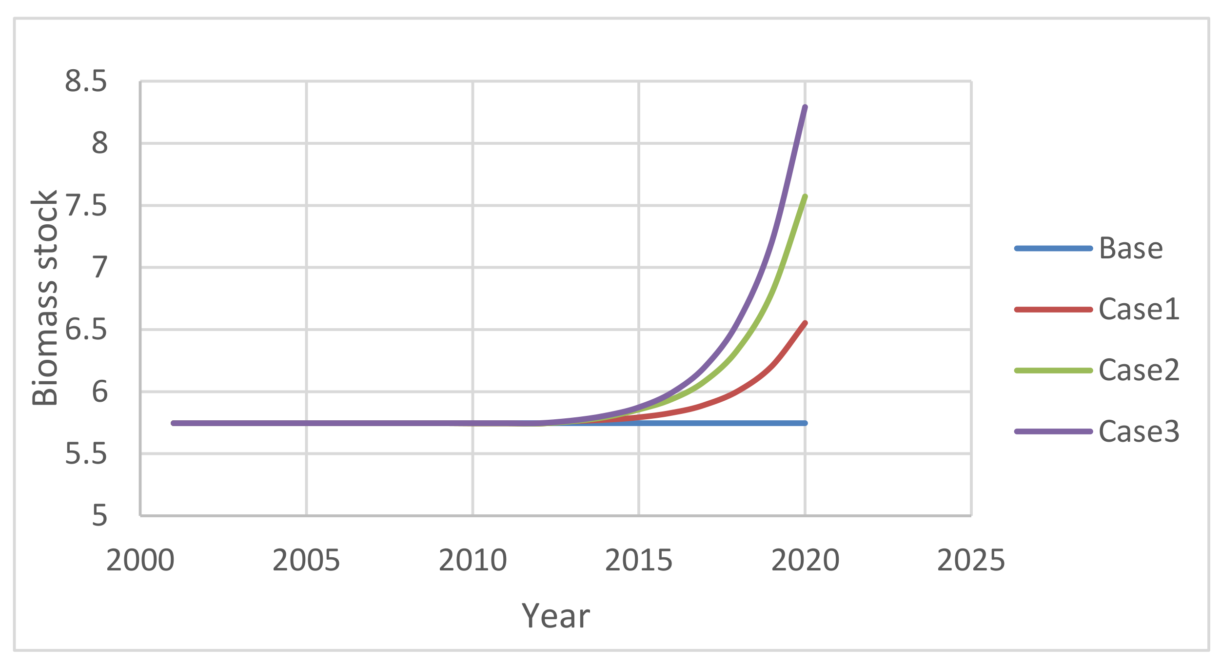
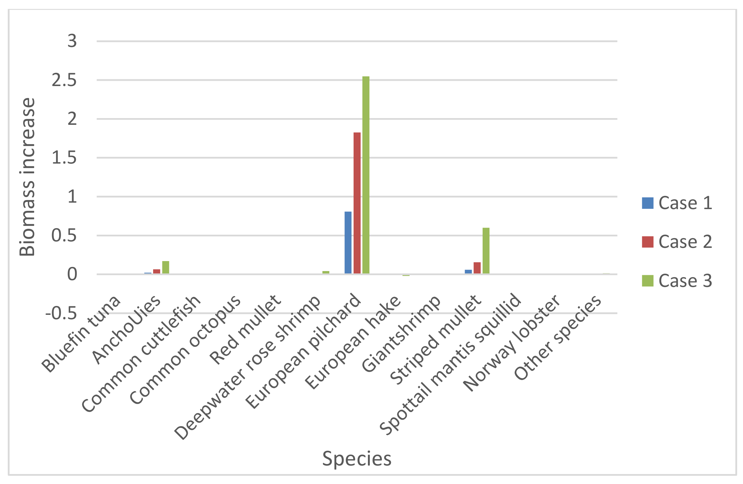
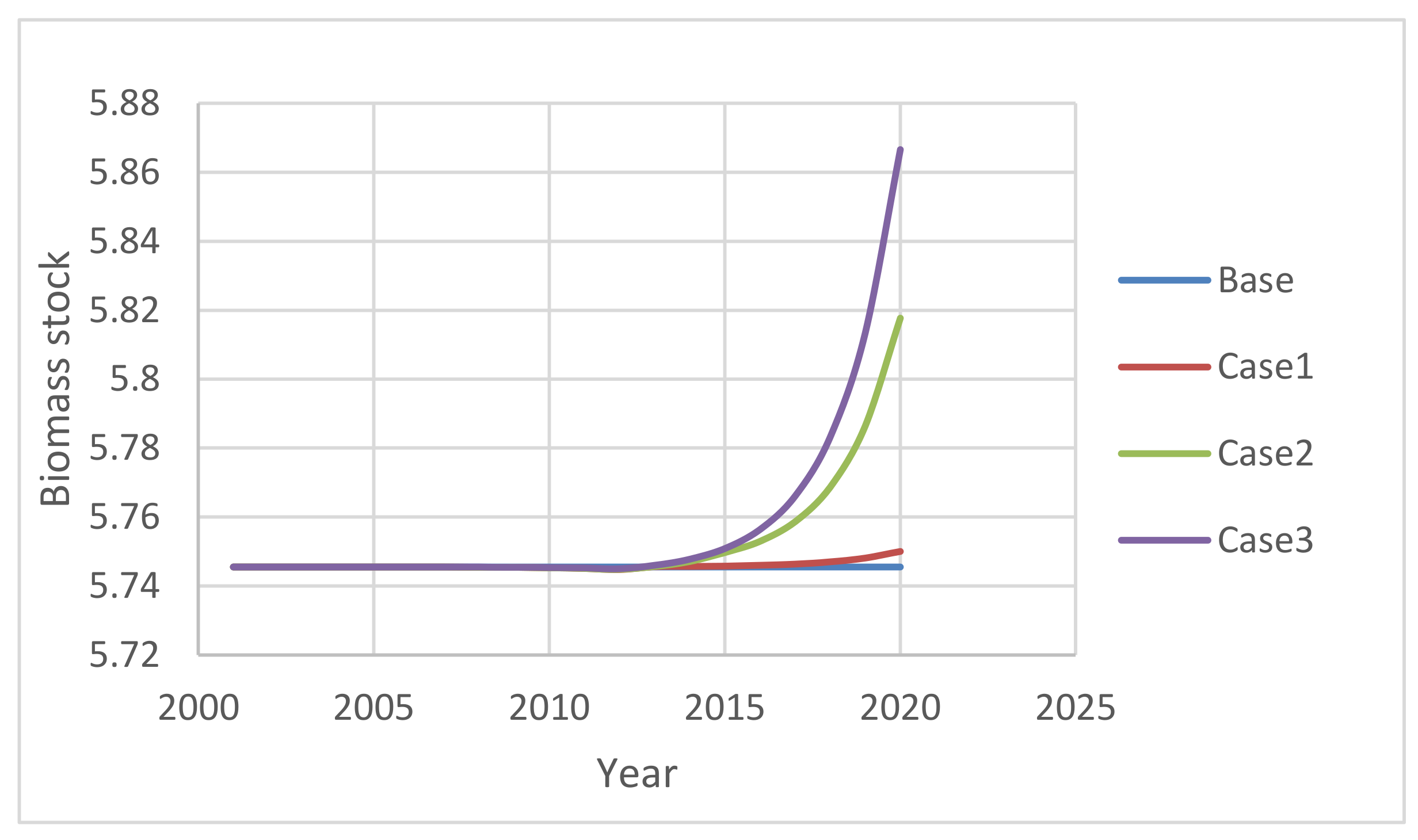
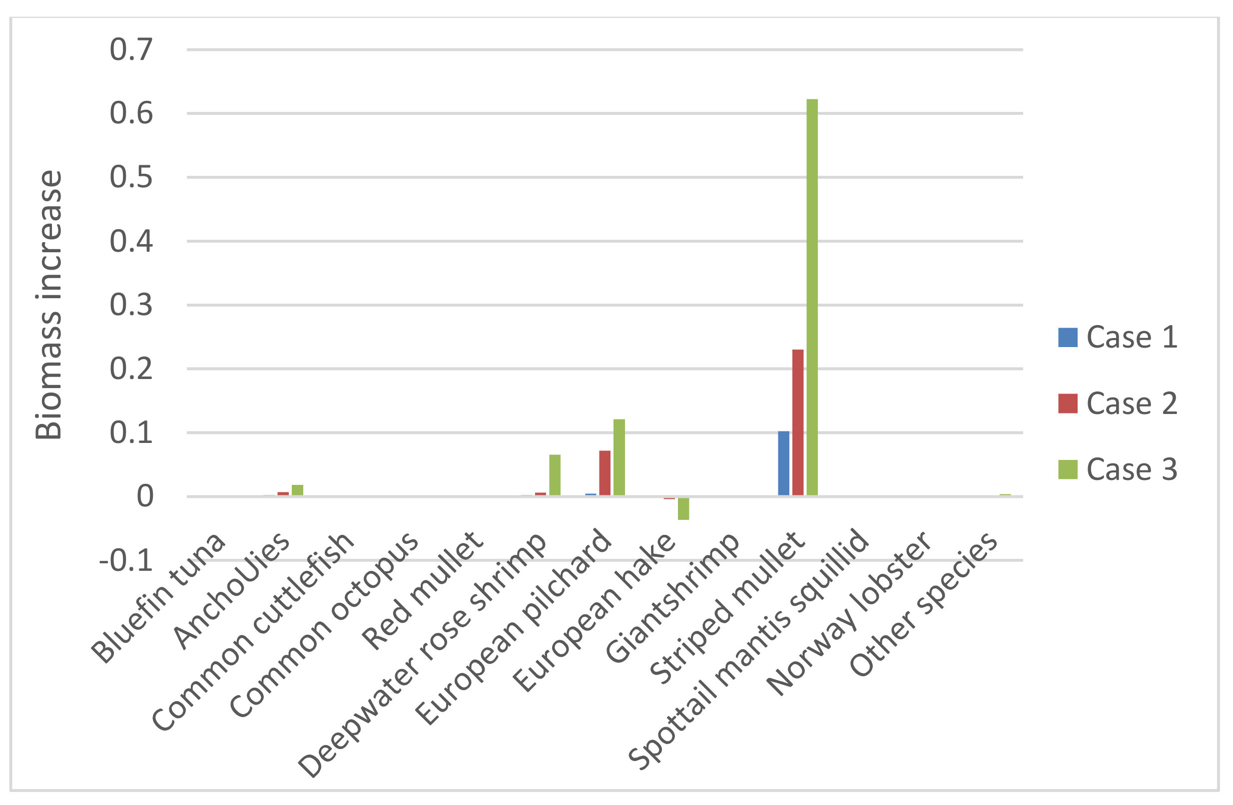
In Scenario 1, we assume a consumption tax on European pilchards to depress demands and thus harvesting. A tax that doubles the original tax rate is assumed to start from the year 2012—12 years since the base year 2001—and thereafter ran three different cases. Case 1 will execute the tax just for one year, Case 2 will execute the tax for three consecutive years and the Case 3 will execute the tax for all the years from 2012 to 2030. Figure 4 show that the tax in each case can push up biomass stock of European pilchards for all the periods from 2012. Figure 5 compares the biomass stock in 2020 to the level in 2001; obviously, the biomass stock of European pilchard will have remarkable increases while other species may increase or decrease slightly.
Scenario 2 considers a production tax directly exercised on the métier of purse seiners, the only métier responsible for harvesting European pilchard. By the data, the existing production tax rate on the métier is small at 1.5%. In this scenario, we also double the existing rate of the production tax. Again, the assumed tax will be applied with three different cases, like in Scenario 1. Figure 6 shows that when the tax rate is doubled, the biomass of European pilchard will grow at a moderate pace. However, Figure 7 shows that compared to its 2001 level Striped mullet will increase most through 2020, while European pilchard the second most.
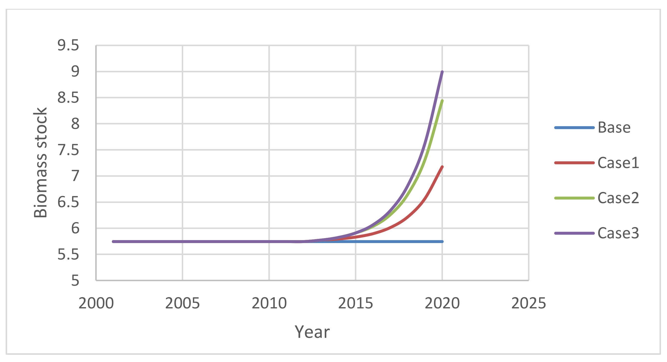
In Scenario 3, we study the Total Allowed Catch (TAC) on European pilchards. The scenario assumes that the catch of European pilchards cannot exceed 75% of the catch in 2001. Figure 8 shows that biomass stock of European pilchards will grow considerably. Like Scenario 1, Figure 9 shows that the biomass stock of European pilchard will increase remarkably from 2001 to 2020, while biomass stocks of other species will almost remain constant. This suggests that TAC is an effective and targeting instrument in the management of fisheries.
It is necessary to mention that there are two additional assumptions with these scenarios. The first assumption is capital reversibility. Normally, capital is regarded to be irreversible [35], and its change depends only on investment and depreciation. In the model, since capital is always fully employed, disinvestment is needed to make the management programs feasible. Thus, we relax the irreversibility of capital by allowing the capital of the métiers to be reversible. This means the harvester can reduce its capital stock by not only depreciation and reduced investment but also disinvestment or capacity buy-back. The second assumption associating with the first one assumes government to operate capacity buy-back schemes to help the métiers comply with management schemes.
The limited empirical exercises demonstrate that the model has great potential and flexibility for policy analysis. In particular, it reveals the possible trends in fisheries’ production and the species dynamics for the Salerno fisheries, and finds out that capacity reduction is the key to success of species rescue. It is vital to set up management or policy schemes that can induce harvesters to cut down fishing capacity. Among the three studied instruments, TAC in combination with capacity buy-back can do the best job.
5. Conclusions and Limitations
This model is specifically developed for countries or regions where fisheries are the mainstay of the economy. A slight change in fisheries policy can have a significant macroeconomic impact on these regions, including the employment, income and welfare of households, as well as the GDP and CPI of the economy. However, they lack an integrated method to conduct a quantitative fisheries policy assessment. This model provides a SAM-based, multi-sector, multi-agent and inter-temporal CGE model to solve this specific problem in fisheries economics.
The establishment of this general equilibrium model with a focus on fisheries enables us to adapt various management and policy instruments to evaluate their impact on fisheries, resource protection, poverty reduction, regional economic regeneration and growth, etc. In addition to the price and structural relations, as specified in standard general equilibrium modelling, four new contributions for the fisheries general equilibrium modelling appear in this research. Firstly, the fisheries sector is split into capture, aquaculture and fish-processing sectors—all of which are treated in parallel to other economic sectors. Within the capture fisheries, fishers are further classified into five types of bottom–up harvesters—the métier. Secondly, fisheries households are separately considered apart from general, non-fisheries households according to income source. This arrangement gives the possibility to assess fisheries society’s benefits and costs under different fisheries management and economic policies. Thirdly, fishing activity is connected to biological systems to capture dynamic interactions between capture and biomass production. The idea here is that fishing activity affects biomass stock, which changes the CPUE (Catch Per Unit Effort) values, which, in turn, have an impact on fishing activity. Fourthly, the model takes forward-looking investment decisions on sector development to project the future situations, and is based on the regional SAM (Social Accounting Matrix) to calibrate the parameters.
Linking the economic and ecological systems in the model is a new attempt, which captures the endogenous interactions of the two systems. For simplicity, in this research we provisionally present the ecological system with surplus production models. It is desirable to model the ecological system in a more detailed and in-depth way. However, we do not recommend doing this in the CGE model, because the task would be beyond an economist’s ability and add more complexity to the modelling work. Instead, we would prefer to have the economic and biological models developed independently and sophisticatedly and continue to link them externally.
Since the contribution of this paper is mainly to propose a new integrated fisheries management tool, we only took Salerno as a simple example in the empirical analysis, setting only three fisheries policy scenarios, namely, a consumption tax on pilchards species, a production tax on the harvester of the species and a Total Allowed Catch (TAC) on the species. The purpose of this simple example is to try to confirm that the model can be applied to fisheries policy. The actual fisheries policy is more complex, but it can also be stimulated in this model, which will not be described in detail in this paper. In addition, in the analysis of the results, the paper only presents the changes in the biomass stock without showing the changes in the economic indicators. This model will have greater potential for application to other fishing countries or regions in the future.
One of the limitations of this study is that the model is not suitable for developed countries and regions or landlocked regions where the share of fisheries in GDP is so tiny that the macroeconomic impact of fisheries on them is negligible compared to other significant industries. For such research objects, it is suggested to apply a partial equilibrium model for the fishery policy and management.
6. Policy Implications
All coastal countries in the world are facing a common problem of overexploitation of marine resources. The sustainable development of fisheries is a significant issue that needs to be addressed urgently nowadays. The formulation of fisheries policy and management pursue the balance between short-term interests and long-term benefits. From the perspective of economic rationality, consumers pursue utility maximization. However, it will affect the recovery and sustainable development of fisheries. For example, the EU’s common fisheries policy has undergone several reforms. There is a contradiction between fisheries resources and harvesting capacity, for lacking some accurate scientific method to evaluate the fisheries policy. The biological simulation model cannot satisfactorily solve the problem of the trade-off between economic and ecological resources. Preceding fisheries policies led to poor implementation and excessive fishing problems. In short, although overfishing brings short-term economic development, it still brings the problem of depletion of marine living resources. In recent years, improving the regulatory framework for protecting sustainable fisheries development becomes the focus of fisheries research. However, an innovative integrated model that can scientifically assess fisheries policies is also needed, which necessarily includes key decision variables such as the fishing capacity and number of fishing vessels, fisheries subsidies, total allowable catching quota and maximum sustainable catch. It can help to measure the ecological and economic impact. In addition, for individual fishing countries or regions, a computable general equilibrium model of fisheries provides more detailed scientific support for formulating their fisheries policies. With sufficient data on the ecological and economic aspects of fisheries, we can construct the SAM tables of a specific region; this computable general equilibrium model can be built to perform economic simulations of fisheries policy. Taking the fisheries policies as an external shock input in the model, the optimal decision solution can be solved for each period. This provides science-based decision-making for long-term fisheries policy development and effectively avoids the problem of overfishing in fisheries.
Author Contributions
Conceptualization, H.P. and P.F.; methodology, H.P.; software, H.P.; validation, C.F. and L.M.; formal analysis, E.C.; investigation, C.F.; resources, L.M.; data curation, V.P.; writing—original draft preparation, H.P.; writing—review and editing, Q.D.; visualization Q.D.; supervision, H.P.; project administration, P.F.; funding acquisition, H.P. and P.F. All authors have read and agreed to the published version of the manuscript.
Funding
This work has also been carried out with the financial support of the Commission of the European Communities Fifth Framework Programme, QLRT-2000-02277 “Development of new tools and models to evaluate the contribution of aquaculture and fishing activities to the development of coastal areas and their socio-economic interactions with other competing sectors” (PECHDEV). The study is funded by the National Foreign Expert Project of China, Ministry of Science and Technology of China (Grant no. G2021111012L).
Institutional Review Board Statement
Not applicable.
Informed Consent Statement
Not applicable.
Data Availability Statement
The data is from the PECHDEV project.
Acknowledgments
The co-authors thank the EU for their financial support. It does not necessarily reflect the Commission’s views and in no way anticipates future policy in this area. The co-authors also thank the National Foreign Expert Project of China.
Conflicts of Interest
The authors declare no conflict of interest.
References
- Goti-Aralucea, L.; Fitzpatrick, M.; Döring, R.; Reid, D.; Mumford, J.; Rindorf, A. Overarching sustainability objectives overcome incompatible directions in the Common Fisheries Policy. Mar. Policy 2018, 91, 49–57. [Google Scholar] [CrossRef]
- Lizaso, J.L.S.; Sola, I.; Guijarro-García, E.; Bellido, J.M.; Franquesa, R. A new management framework for western Mediterranean demersal fisheries. Mar. Policy 2019, 112, 103772. [Google Scholar]
- De Boni, A.; Roma, R.; Palmisano, G.O. Fishery policy in the European Union: A multiple criteria approach for assessing sustainable management of Coastal Development Plans in Southern Italy. Ocean. Coast. Manag. 2018, 163, 11–21. [Google Scholar] [CrossRef]
- Seeteram, N.; Bhat, M.; Pierce, B.; Cavasos, K.; Die, D. Reconciling economic impacts and stakeholder perception: A management challenge in Florida Gulf Coast fisheries. Mar. Policy 2019, 108, 103628. [Google Scholar] [CrossRef]
- Byron, C.J.; Jin, D.; Dalton, T.M. An Integrated ecological–economic modeling framework for the sustainable management of oyster farming. Aquaculture 2015, 447, 15–22. [Google Scholar] [CrossRef]
- Gordon, H.S. The economic theory of a common-property resource: The fishery. J. Political Econ. 1954, 62, 124–142. [Google Scholar] [CrossRef]
- Lofgren, H.; Harris, R.; Robinson, S. A Standard Computable General Equilibrium (CGE) Model in GAMS; Trade and Macroeconomics Discussion Paper No. 75; International Food Policy Research Institute: Washington, DC, USA, 2001. [Google Scholar]
- Clark, C.W.; Munro, G.R. The economics of fishing and modern capital theory: A simplified approach. J. Environ. Econ. Manag. 1975, 2, 92–106. [Google Scholar] [CrossRef]
- Clark, C.W. Mathematical Bioeconomics: The Optimal Management of Renewable Resources; Wiley-Interscience: New York, NY, USA, 1976. [Google Scholar]
- Clark, C.W.; Clarke, F.H.; Munro, G.R. The optimal exploitation of renewable resource stocks: Problems of irreversible investment. Econometrica 1979, 47, 25–47. [Google Scholar] [CrossRef]
- Brites, N.M.; Braumann, C.A. Fisheries management in random environments: Comparison of harvesting policies for the logistic model. Fish. Res. 2017, 195, 238–246. [Google Scholar] [CrossRef]
- Pei, Y.; Chen, M.; Liang, X.; Li, C. Model-based on fishery management systems with selective harvest polices. Math. Comput. Simul. 2018, 156, 377–395. [Google Scholar] [CrossRef]
- Van Dijk, D.; Hendrix, E.M.T.; Haijema, R.; Groeneveld, R.A.; van Ierland, E.C. On solving a bi-level stochastic dynamic programming model for analyzing fisheries policies: Fishermen behaviour and optimal fish quota. Ecol. Model. 2014, 272, 68–75. [Google Scholar] [CrossRef]
- Tokunaga, K.; Ishimura, G.; Iwata, S.; Abe, K.; Otsuka, K.; Kleisner, K.; Fujita, R. Alternative outcomes under different fisheries management policies: A bioeconomic analysis of Japanese fisheries. Mar. Policy 2019, 108, 103646. [Google Scholar] [CrossRef]
- Rosa, R.; Costa, T.; Mota, R.P. Incorporating economics into fishery policies: Developing integrated ecological-economics harvest control rules. Ecol. Econ. 2022, 196, 107418. [Google Scholar] [CrossRef]
- Seung, C.K.; Waters, E.C. A review of regional economic models for fisheries management in the U.S. Mar. Resour. Econ. 2006, 21, 101–124. [Google Scholar] [CrossRef]
- Seung, W.C.K. Impacts of Recent Shocks to Alaska Fisheries: A Computable General Equilibrium (CGE) Model Analysis. Mar. Resour. Econ. 2010, 25, 155–183. [Google Scholar]
- Carvalho, N.; Rege, S.; Fortuna, M.; Isidro, E.; Edwards-Jones, G. Estimating the impacts of eliminating fisheries subsidies on the small island economy of the Azores. Ecol. Econ. 2011, 70, 1822–1830. [Google Scholar] [CrossRef] [Green Version]
- Jin, D.; Hoagland, P.; Dalton, T.M.; Thunberg, E.M. Development of an integrated economic and ecological framework for ecosystem-based fisheries management in New England. Prog. Oceanogr. 2012, 102, 93–101. [Google Scholar] [CrossRef] [Green Version]
- Da-Rocha, J.M.; Prellezo, R.; Sempere, J.; Taboada Antelo, L. A dynamic economic equilibrium model for the economic assessment of the fishery stock-rebuilding policies. Mar. Policy 2017, 81, 185–195. [Google Scholar] [CrossRef] [Green Version]
- Eichner, T.; Pethig, R. Pricing the ecosystem and taxing ecosystem services: A general equilibrium approach. J. Econ. Theory 2009, 144, 1589–1616. [Google Scholar] [CrossRef] [Green Version]
- Eichner, T.; Pethig, R. Harvesting in an integrated general equilibrium model. Environ. Resour. Econ. 2007, 37, 233–252. [Google Scholar] [CrossRef] [Green Version]
- Finnoff, D.; Tschirhart, J. Linking dynamic economic and ecological general equilibrium models. Resour. Energy Econ. 2005, 30, 91–114. [Google Scholar] [CrossRef]
- Kaplan, I.C.; Leonard, J. From krill to convenience stores: Forecasting the economic and ecological effects of fisheries management on the US West Coast. Mar. Policy 2012, 36, 947–954. [Google Scholar] [CrossRef]
- Santiago, J.L.; Surís-Regueiro, J.C. An applied method for assessing socioeconomic impacts of European fisheries quota-based management. Fish. Res. 2018, 206, 150–162. [Google Scholar] [CrossRef]
- Dhk, A.; Chang, K. Economic contributions of wild fisheries and aquaculture: A social accounting matrix (SAM) analysis for Gyeong-Nam Province, Korea. Ocean. Coast. Manag. 2020, 188, 105072. [Google Scholar]
- Wang, Y.; Hu, J.; Pan, H.; Failler, P. Ecosystem-based fisheries management in the Pearl River Delta: Applying a computable general equilibrium model. Mar. Policy 2020, 112, 103784. [Google Scholar] [CrossRef]
- Devarajan, S.; Go, S. The simplest dynamic general-equilibrium model of an open economy. J. Policy Modeling 1998, 20, 677–714. [Google Scholar] [CrossRef]
- Robinson, S.; Yunez-Naude, A.; Hinojosa-Ojeda, R.; Lewis, J.; Devarajan, S. From stylized to applied models: Building multisector CGE models for policy analysis. N. Am. J. Econ. Financ. 1999, 10, 5–38. [Google Scholar] [CrossRef]
- Burt, O.R.; Cummings, R.G. Production and investment in natural resource industries. Am. Econ. Rev. 1970, 60, 576–590. [Google Scholar]
- PECHDEV Final Report, A Computable General Equilibrium (CGE) Model in Fisheries: Policy Analysis with Evidence from Five European Regions; EU Funded RTD Project QLRT-2000-02277: Development of New Tools and Models to Evaluate the Contribution of Aquaculture and Fishing Activities to the Development of Coastal Areas and Their Socio-economic Interactions with Other Competing Sectors; Failler, P. (Ed.) European Union: Maastricht, The Netherlands, 2007. [Google Scholar]
- Pella, J.J.; Hilborn, R.; Walters, C.J. Quantitative Fisheries Stock Assessment: Choice, Dynamics and Uncertainty; Routledge Chapman & Hall: London, UK, 1992. [Google Scholar]
- Schaefer, M.B. Some aspects of the dynamics of populations important to the commercial marine fisheries. Bull. Math. Biol. 1991, 53, 253–279. [Google Scholar] [CrossRef]
- Failler, P.; Pan, H. Global value, full value, societal costs; capturing the true cost of destroying the marine ecosystems. Soc. Sci. Inf. 2007, 46, 109–134. [Google Scholar] [CrossRef]
- Arrow, K.J. Optimal Capital Policy with Irreversible Investment. In Value, Capital, and Growth: Papers in Honour of Sir John Hicks; Wolfe, J.N., Ed.; Edinburgh University Press: Edinburgh, Scotland, 1968; pp. 1–20. [Google Scholar]
Figure 1.
The nested scheme of consumption.

Figure 2.
The nested production scheme for a top–down non-fisheries producer.

Figure 3.
The nested production scheme for bottom–up fisheries producer.

Figure 4.
Changes in biomass stock under consumption taxes.

Figure 5.
Biomass increase from 2001 to 2020 under consumption taxes.

Figure 6.
Changes in biomass stock under production taxes.

Figure 7.
Biomass increase from 2001 to 2020 under production taxes.

Figure 8.
Changes in biomass stock under quota.

Figure 9.
Biomass increase from 2001 to 2020 under quotas.


Table 1.
Biological data on the species and growth functions.
| Species | φ | r | Cap (k ton) | BM (k ton) | BM/Cap | Model |
|---|---|---|---|---|---|---|
| Bluefin tuna | 2.53 | 0.07 | 556.21 | 204.03 | 36.68% | Fox |
| Anchovies | 8.42 | 0.03 | 19.96 | 7.34 | 36.79% | Fox |
| Common cuttlefish | 23.47 | 0.15 | 2.38 | 0.87 | 36.79% | Fox |
| Common octopus | 23.93 | 0.06 | 2.77 | 1.02 | 36.79% | Fox |
| Red mullet | 6.91 | 0.03 | 0.49 | 0.18 | 36.76% | Fox |
| Deepwater rose shrimp | 1.24 | 0.47 | 0.97 | 0.17 | 17.25% | Logistic |
| European pilchard | 3.97 | 0.02 | 157.24 | 5.75 | 3.65% | Fox |
| European hake | 1.04 | 0.47 | 1.20 | 0.12 | 10.32% | Logistic |
| Giant red & blue shrimp | 0.73 | 0.47 | 0.78 | 0.21 | 27.14% | Logistic |
| Striped mullet | 1.73 | 0.44 | 0.89 | 0.13 | 15.12% | Logistic |
| Spottail mantis squillid | 10.40 | 0.28 | 1.53 | 1.04 | 67.88% | Fox |
| Norway lobster | 1.52 | 0.02 | 12.64 | 0.93 | 7.35% | Fox |
| Other species | 4.96 | 0.08 | 222.33 | 81.79 | 36.79% | Fox |
Table 2.
Elasticity of substitution.
| Elasticity | Value | Equation |
|---|---|---|
| ρgf | 0.75 | Non-fishery productions |
| ρio | 0.25 | Production of composite intermediate product |
| ρaa | 0.75 | Production of composite agro and aqua product |
| ρeis | 0.5 | Production of composite energy, industrial and service product |
| ρaqu | 0.75 | Production of composite aquatic product |
| ρCET | −0.5 | CET function |
| ρAMT | 0.5 | Armington function |
| σaa | 0.75 | Consumption of agricultural and aquatic product |
| σaqu | 0.75 | Consumption of aquatic product |
Publisher’s Note: MDPI stays neutral with regard to jurisdictional claims in published maps and institutional affiliations. |
© 2022 by the authors. Licensee MDPI, Basel, Switzerland. This article is an open access article distributed under the terms and conditions of the Creative Commons Attribution (CC BY) license (https://creativecommons.org/licenses/by/4.0/).
Share and Cite
MDPI and ACS Style
Pan, H.; Failler, P.; Du, Q.; Floros, C.; Malvarosa, L.; Chassot, E.; Placenti, V. An Inter-Temporal Computable General Equilibrium Model for Fisheries. Sustainability 2022, 14, 6444. https://doi.org/10.3390/su14116444
AMA Style
Pan H, Failler P, Du Q, Floros C, Malvarosa L, Chassot E, Placenti V. An Inter-Temporal Computable General Equilibrium Model for Fisheries. Sustainability. 2022; 14(11):6444. https://doi.org/10.3390/su14116444
Chicago/Turabian StylePan, Haoran, Pierre Failler, Qianyi Du, Christos Floros, Loretta Malvarosa, Emmanuel Chassot, and Vincenzo Placenti. 2022. "An Inter-Temporal Computable General Equilibrium Model for Fisheries" Sustainability 14, no. 11: 6444. https://doi.org/10.3390/su14116444
Note that from the first issue of 2016, this journal uses article numbers instead of page numbers. See further details here.