1. Introduction
Aero-engine thermodynamic models are widely used in engine design [
1], development [
2] and monitoring [
3]. However, in the field of military turbofans, thermodynamic models suffer from serious non-convergence [
4,
5], mainly due to the following reasons.
First, the accuracy of the component characteristic maps is low, and the smoothness is poor due to individual differences in engine manufacturing and assembly tolerances [
6], which may lead to inaccuracy and even interruption of the thermodynamic modeling process.
In addition, unlike civil aviation engines, military turbofans sometimes work near the boundary of the flight envelope to fully use the engine to its maximum potential in some situations, such as vertical climbing and fast maneuvering [
7,
8]. In this case, the thermodynamic model tends to iterate beyond the flight envelope and component characteristic maps, leading to model non-convergence.
To solve the above problems, component characteristic map fitting and smoothing methods are introduced. Kong et al. [
9] proposed a polynomial scaling method to correct the component characteristic maps at multiple operation points, and the accuracy of the off-design points within the flight envelope was greatly improved. Kong et al. [
10,
11] generated component maps using a cubic fitting method and genetic algorithms. More-accurate and smoother maps can be acquired through the optimization process. Li et al. [
12,
13] introduced a nonlinear, multiple-point performance adaptation approach using a genetic algorithm to improve the performance prediction accuracy of gas turbine engines at different off-design conditions by calibrating the engine performance models against available test data. The adaptation approach was applied to a gas turbine engine, and the experiment demonstrated a significant improvement in the performance evaluation accuracy in off-design operating conditions. Tsoutsanis et al. [
14] introduced a new compressor map fitting and modeling method to simultaneously determine the best elliptical curves to a set of compressor map data. The results verified the capabilities of their method in refining existing engine performance models to different modes of gas turbine operation. Kim et al. [
15] proposed a two-step adjustment of the scale factors for overall and local performance parameters. The result of the model showed improved prediction in both the overall and local performance parameters.
These scaling and curve fitting methods can correct component maps toward the operating space of certain engines, especially in design points. However, the number of corrected variables is too few to cover all of the flight envelope.
Improving the accuracy and generalization capability of the characteristic map can improve the convergence of the model to some extent. However, even though the component maps are well-smoothed and generalized, the iteration process of the thermodynamic model is easy to run outside the characteristic maps in some conditions where the engine is operating near the flight envelope, resulting in non-convergence.
With the recent development of neural networks, there are many different domains where advanced artificial intelligence approaches have been applied as solution approaches, such as online learning [
16], scheduling [
17], multi-objective optimization [
18], transportation [
19], medicine [
20], and data classification [
21]. Neural network-based methods can correct component maps in such a data-driven way that smoother and more-generalized maps can be acquired. Yu et al. [
22] proposed a three-layer neural network to predict a compressor map using data provided by manufacturers. Ghorbanian and Gholamrezaei [
23] tested various neural networks to predict compressor performance using experimental data and achieved excellent agreement between the predictions and the experimental data using a multilayer perceptron network.
Neural network-based methods improve convergence through forward calculation. However, most neural networks take component characteristic modeling as a pure regression problem, ignoring dynamic constraints during the components’ working process. In this case, these methods can only fit limited data from the test rig and cannot achieve high accuracy with a large number of flight data.
Aiming to solve the non-convergence problem of traditional thermodynamic models and the mismatch between neural network models and the engine working process, a thermodynamically oriented and neural network-based hybrid model for military turbofans is proposed. The iterative process of the thermodynamic model is transformed into a feed-forward calculation of the hybrid model to improve convergence. Moreover, a multi-objective loss function describing the component co-working process is proposed to help the hybrid model converge toward the real thermodynamic state space of military turbofans.
The main contributions of our work lie in the following aspects:
A new component-level neural network structure is proposed that transforms the iterative process of the thermodynamic model into the feed-forward process of the neural network to improve convergence and computational efficiency of the model.
A multi-objective loss function based on component co-working is proposed to direct the neural network model to converge toward the physical thermodynamic process.
Fusion training of multiple data sources is established to train the hybrid model with good convergence and high computational accuracy.
The remaining sections are organized as follows. Firstly, the modeling process of the traditional thermodynamic model for aero-engines is briefly introduced; then, the thermodynamically oriented and neural network-based hybrid model for military turbofans is proposed; finally, the proposed model is tested on flight data and compared with other state-of-the-art methods.
3. Proposed Hybrid Model
The proposed hybrid model is comprised of the following three phases.
First, a component-level neural network is built to transform the iterative process of traditional thermodynamic models into the forward process of the network’s structure. The component nets are joined according to the gas path relationship, and the component maps are replaced with the weights in the component nets, which can be adjusted in the training process. Thus, the non-convergence caused by the component maps can be overcome.
Then, a multi-objective loss function describing the degree of deviation from components’ collaborative working state is proposed. By transforming the equilibrium equations in thermodynamic models into equilibrium loss, the multi-objective loss function can direct the training process to converge towards the turbofan thermodynamics.
Last, a multi-data fusion training process is introduced to gradually guide the hybrid model to converge towards the on-wing working state of the turbofans with the help of the simulation pre-training and flight data training phase.
The following describes the above three phases in turn.
3.1. Component Level Neural Network
The iterative process around the flight envelope boundary (
Figure 2) of the thermodynamic model can easily run outside the components’ characteristic maps, which is the key reason for non-convergence. To solve this problem, the proposed hybrid model takes a component-level neural network to transform the iterative process into the feed-forward process.
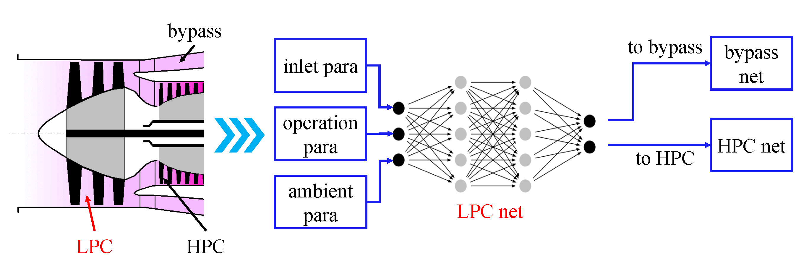
Figure 3 illustrates the structure of the fan net in the component-level neural network. From the gas connection relationship, the LPC is a single-input, dual-output channel. Therefore, the inlet parameters of the fan module (such as total inlet temperature, total pressure, etc.) are only one-way, while the outlet parameters are two-way as they are connected to the inlet parameters of the bypass net and the low pressure compressor net. To determine the outlet parameters of the fan module, the operating parameters of the fan (e.g., speed, flow rate, etc.) should also be input into the module.
Once the above connections have been determined, the actual gas flow of the fan (the left part of
Figure 3) can be transformed into a neural network module oriented towards its thermodynamic processes (the right part of
Figure 3), thus completing the representation of the operating process of the fan.
All component nets are similar in that they have four fully connected network layers (
Figure 4), with the Rectified Linear Unit (ReLU) activation function in the first three. The component net inputs are the station parameters of the inlet and the operating parameters. The outputs are the station parameters of the component outlet. Therefore, the outputs of one component are parts of the inputs of downstream components.
There are 128, 512, 512 and 128 neutrons in the first, second, third and fourth layers, respectively, of the HPC, burner, HPT, LPT, bypass and nozzle net; there are 128, 512, 512 and 256 neutrons for these layers, respectively, in the LPC net because of its dual exits, and 256, 512, 512 and 128 neutrons, respectively, in the LPC net because of its dual inlets. The number of neutrons in each layer was determined through a hyper-parameter validation experiment where 20 groups of different neutron numbers settings were compared. At last, the above setting showed the highest accuracy.
The general structure of the proposed component-level neural network is illustrated in
Figure 5. The parameters inside the dashed line are the inputs to the hybrid model.
3.2. Multi-Objective Loss Function
In the traditional thermodynamic model, equilibrium Equations (
1)–(
4) are solved by an iterative method such as the Newton-Raphson method. However, because the iterative process has been replaced by the feed-forward process of the hybrid model, the equilibrium state for engine components collaboratively working is difficult to satisfy only by the traditional mean square error loss for the neural network.
To address the above problem, a multi-objective loss function based on component co-working is proposed. The set of equilibrium equations for component co-working is transformed into a set of corresponding loss functions in the training process of the neural network. The hybrid model is guided to converge in the direction of mass flow equilibrium, pressure equilibrium and power equilibrium through the training process to complete the modeling of component co-working.
The mass flow equilibrium loss is defined as follows.
where
M is the number of stations in the aero-engine, and
are the air mass flow, the total temperature, the total pressure, Mach number and the area of the
ith station, respectively, for each station separately.
is the mass flow equation in aerodynamics:
The pressure equilibrium loss is defined as follows.
where
is the static pressure of the nozzle throat calculated by the station parameters,
is the static pressure calculated by the ambient pressure, and
and
are the static pressures of the mixer inlet from the bypass and the core path, respectively, calculated by the station parameters.
The power equilibrium loss is defined as follows.
where
and
are the mechanical drive efficiency of the HPT and LPT, respectively,
and
are the output work of the HPT and LPT, respectively, that can be computed by the state parameters,
and
are the required work of the compressors and
and
is the power extraction volume from the HPT and LPT, respectively.
Combined with the mean squared loss, the above losses are accumulated according to certain weights to form the final multi-objective loss function.
where
is the root mean squared loss that measures the difference between the actual station parameters
and the estimated values
of the neural network model.
The different weights in Equation (
10) measure the compromise between the station parameters and the components’ co-working process in directing the training process. In our experiment, these weights are determined by a grid searching process: different weight groups are set to get the modeling error in the validation set. Finally, the weights group that achieves the lowest error is chosen as the final weights.
3.3. Multi-Data-Source Fusion Training
Because there are few station parameters recorded in flight data, the constraint of the station parameter loss is too weak to make the network converge quickly and precisely. To increase the number of station parameters and to make optimization more effective, a simulation data pre-training phase is proposed to model approximate component characteristics. Then, the hybrid model is trained by the flight data to correct the component characteristics. The multi-data-source fusion training process is illustrated in
Figure 6.
3.3.1. Simulation Data Pre-Training Phase
The simulation data pre-training phase is carried out in the following process.
First, many inputs required by the thermodynamic model—usually the rotor speed of the high-pressure shaft (denoted as N2), the total temperature of the LPC inlet (denoted as T2), the total pressure of the LPC inlet (denoted as P2), the ambient pressure (denoted as Pamb)—are generated randomly in a reasonable scope.
where the subscript
i denotes the
ith sample.
Then, these variables are input into the thermodynamic model to calculate all variables and station parameters required by the hybrid model’s inputs and outputs.
where
is the the low-pressure shaft rotor speed of the
ith sample,
is the fuel mass flow of the
ith sample and
are the station parameters required by the hybrid model’s outputs.
When the inputs and outputs required by the hybrid model are all computed, the dataset can be generated. In , is the input vector of the ith sample for the hybrid model and is the station parameter that is the desired output vector of the hybrid model.
At last, the hybrid model is trained by
using the loss function Equation (
10) with the gradient descend method. If trained properly, the hybrid model can learn approximate component characteristics and also incorporate thermodynamic models in calculating the station parameters.
3.3.2. Flight Data Training Phase
Because the simulation data is generated by the thermodynamic model, after the simulation data pre-training phase, the accuracy of the hybrid model cannot be higher than the thermodynamic model. To improve accuracy, flight data training is proposed to correct component characteristics by adjusting the network’s weights using flight data.
First, a quasi steady state is defined where the amplitude of N1 is less than for 3 s without consideration of the fluctuation of other variables, such as Mach number, altitude and inlet temperature. This is a very relaxed quasi-steady-state determinant condition and poses great challenges to performance calculation.
Next, quasi steady state points are extracted from a specific engine over a period of time to form dataset .
The multi-objective loss function introduced in
Section 3.2 is used to train the hybrid model. The main difference lies in the root mean squared loss. Because there are only a few station parameters in the flight data, not all the station parameters output by the hybrid model will contribute to the loss. The root mean square loss of the flight data training phase is modified as:
where
extracts the network’s outputs corresponding to
in the flight data to compute the loss.
Then, the hybrid model is trained using the gradient descent method. After the flight data training phase, component characteristics are corrected using the on-wing flight data. Thus, the modeling accuracy will be higher than the network only trained by the simulation dataset and thermodynamic models.
In these three phases, the component-level neural network guarantees that the hybrid model follows the turbofan’s airflow process and overcomes the non-convergence in the thermodynamic models; the multi-objective loss function ensures the hybrid model converges toward the component’s co-working state; the multi-data source fusion training improves the accuracy of the hybrid model by considering the correction provided by the flight data.
4. Test Case
In this section, the accuracy of the hybrid model is tested in the flight data gathered from a two-spool turbofan over a period of time.
Table 1 shows the flight data and the notation ∗ represents the value of the corresponding parameter that is not convenient to show for confidentiality reasons. Mass flow can be evaluated using the flight Mach number, the inlet parameters and the inlet area with the mass flow equation in aerodynamics (Equation (
7)). The pressure ratio is only measured for the engine control but not recorded in the flight data.
The input data of the hybrid model include the rotor speed of the low pressure shaft (denoted as N1), the rotor speed of the high pressure shaft (denoted as N2), the mass flow of fuel (denoted as
), the total temperature of the LPC inlet (denoted as T2), the total pressure of the LPC inlet (denoted as P2) and the ambient pressure (denoted as Pamb). All these data can be acquired from the flight data. Wild value processing and data augmentation [
27] are used to improve the quantity of flight data. There is only one station parameter—the total temperature of the LPT exit (denoted as T6)—recorded in the flight data, so it is used to measure the accuracy of the hybrid model. Two datasets are made for the whole training and testing processes:
is the simulation dataset generated using the thermodynamic model introduced in
Section 3.3.1 and
is gathered as introduced in
Section 3.3.2.
4.1. Simulation Data Pre-Training Results
A total of
groups of
as required by the thermodynamic model are generated using Equation (
12). Then, each group is input into the thermodynamic model to get the corresponding operation and station parameters. Thus,
samples (denoted as
) are generated to train the hybrid model. The input data from
for the hybrid model are N1, N2,
, T2, P2 and Pamb, while the output data are the station parameters. The number of training epochs is 500, the learning rate is
with
decay every 100 epochs, and the batch size is set to 256. Training loss is defined by Equation (
10). Accuracy is measured by the max relative error in all samples of the training set.
where
is a certain station parameter of sample
i, and
is the subscript set of dataset
.
The error trending of turbine exit temperature in the training process is shown in
Figure 7, where the hybrid network converges after about 200 epochs. The training error drops sharply in the first 100 epochs, indicating the appropriateness of the learning rate. In the next 100 epochs, because the learning rate decays by 10%, the training error can be further decreased.
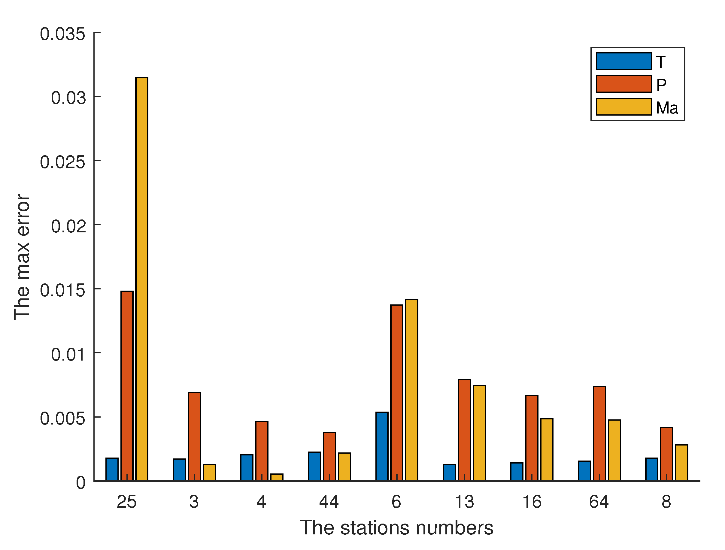
After the simulation data pre-training phase, the max relative errors of the station parameters, the total temperature (denoted as T), the total pressure (denoted as P) and the Mach number (denoted as Ma), are described in
Figure 8. The Mach number error of the LPC exit (denoted as station 25) is 3.2%, which is larger than other stations. This is because there is no Mach number accessible in the flight data as the input of the LPC net. Except for this parameter, the errors of other parameters are less than 1.5%, indicating the effectiveness of the flight data training process.
4.2. Flight Data Training Results
After being trained by the simulation data, the hybrid model is further trained with the flight dataset introduced in
Section 3.3.2. The flight dataset is split into two subsets: the training set
to train the hybrid model and the testing set
to measure the accuracy and generalization of the hybrid model. There are 6970 samples in
and
samples in
.
To compare the performance before and after flight data training, the turbine exit temperature of the flight testing dataset is evaluated using the hybrid model only trained by the simulation data. Then, turbine exit temperature is evaluated using the hybrid model further trained by the flight training dataset. The turbine exit temperature relative-error histogram of the hybrid model trained only by simulation data and further trained by the flight data is illustrated in
Figure 9.
It can be concluded that before being trained by flight data, the turbine exit temperature relative-error distribution is nearly uniform around 6%, with the max relative error reaching 13.8%. This is because the hybrid model is not adjusted by the flight data and can only model the operation of the on-wing turbofans from a thermodynamic perspective. After being further trained by flight data, the turbine exit temperature relative-error is mainly concentrated below 4%, with the max error reaching 7.1%. This is because the component characteristics can be adjusted by optimizing the weights of the component nets according to the flight data, allowing the trained hybrid model to give a more accurate evaluation.
4.3. Comparisons with Thermodynamic Model
Furthermore, the hybrid model trained by the flight training dataset is compared with the thermodynamic model. The thermodynamic model is built on PRopulsion Object Oriented SImulation Software (PROOSIS) that is currently the state-of-the-art tool for aero-engine modeling [
28]. The error distribution histogram comparison between the hybrid model trained by the flight training dataset and the thermodynamic model is shown in
Figure 10.
Similar to the hybrid model not trained by the flight data, the average component-map-based thermodynamic model cannot be customized for individual differences and assembly errors. Thus the max error of the thermodynamic model reaches 7.1%, 5.2% higher than the proposed hybrid model. This also indicates that the hybrid model can extract the engine’s characteristics and degeneration trend from flight data in the flight data training phase to evaluate the station parameters more accurately.
4.4. Comparisons with Neural Network Model
To compare the hybrid model with a pure neural network model, a neural network (denoted as TNN) of equivalent model volume is constructed to predict the turbine exit temperature in the flight data. The neural network has 28 hidden layers, with the same number of hidden dimensions as the hybrid model. The inputs are the same as the hybrid model’s and the output is the turbine exit temperature. The definition of the training loss is defined as Equation (
14). Because no other station parameters can be evaluated by TNN, the thermodynamic loss Equations (
6), (
8) and (
9) cannot be used as loss functions. TNN is trained and tested using the same flight dataset under the same training configurations as the hybrid model. The error-distribution histogram comparison between the hybrid model and TNN is shown in
Figure 11.
Because neither the thermodynamic process nor the component co-working equilibriums are considered in TNN, the TNN network will overfit the training dataset, resulting in a large evaluation error in the testing set. Thus, the max error of TNN reaches 15.8%, which is too high to evaluate the performance of the engine. This also verifies the rationality of the proposed hybrid model’s multi-objective loss function and two-phase training process from another perspective.
4.5. Accuracy Comparisons of Different Methods
The comparisons of different methods are shown in
Table 2. Accuracy is measured by the relative error (RE) between turbine exit temperature (
) in the flight data and its evaluation
by different methods:
Among the table head, ‘mean’ is the mean RE of all testing samples, ‘std’ is the standard deviation of RE, ‘25%’ is the top 25% of RE and ‘max’ is the max RE of all testing samples. In
Table 2, the proposed hybrid model gets the best accuracy in all measurements. In the ‘max’ measurement, the proposed hybrid model is about 5% lower than the thermodynamically based model calculated in PROOSIS, 8% lower than the purely data-driven network with a similar volume, 4% lower than the cubic fitting method [
11] proposed by Kong et al. and 5% lower than the elliptical fitting method [
14] proposed by Tsoutsanis et al.


