
Improved Shallow Landslide Susceptibility Prediction Based on Statistics and Ensemble Learning


Abstract
:1. Introduction
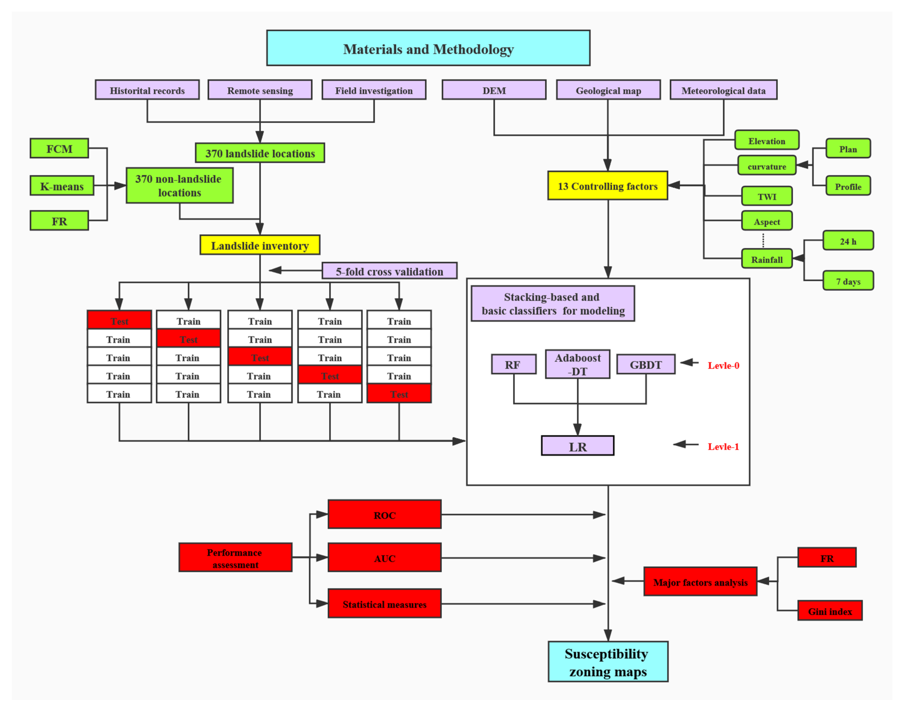
2. Materials
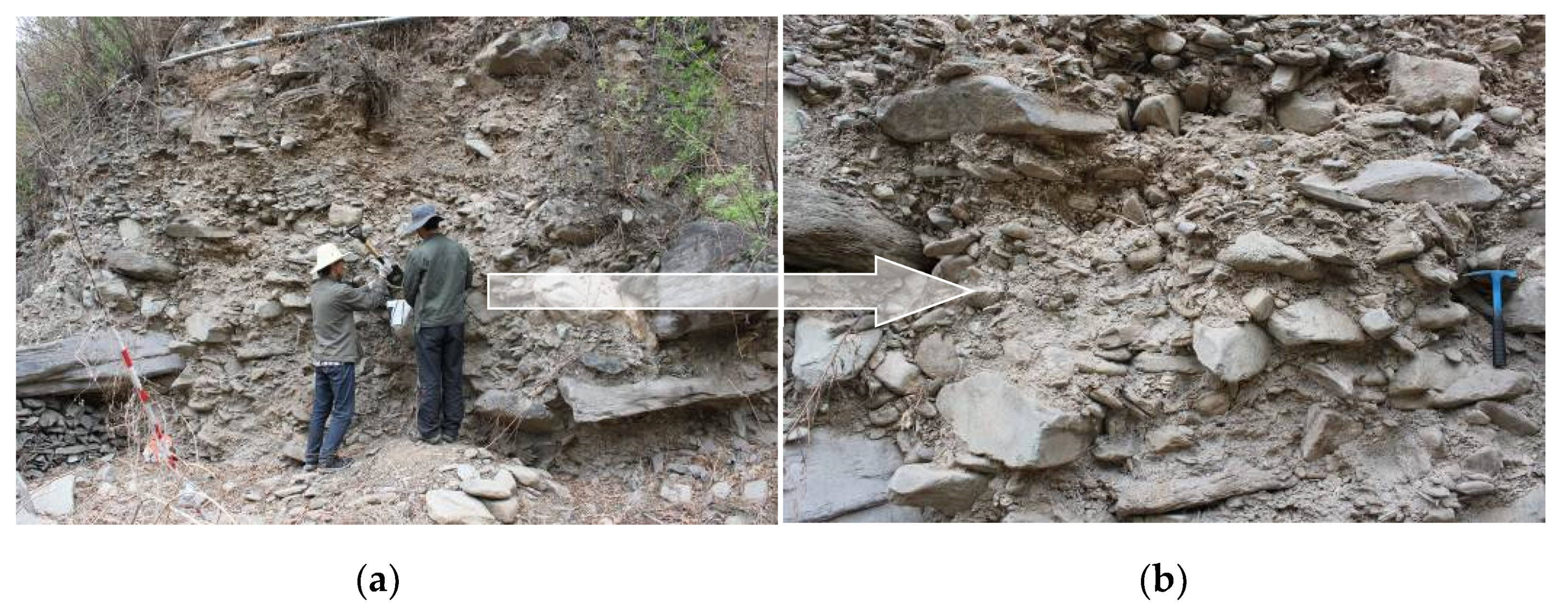
2.1. Study Area
2.2. Data Preparation
2.2.1. Landslide Inventory
2.2.2. Choice of Mapping Units
2.2.3. Conditioning Factors
3. Methods
3.1. Sampling Strategy
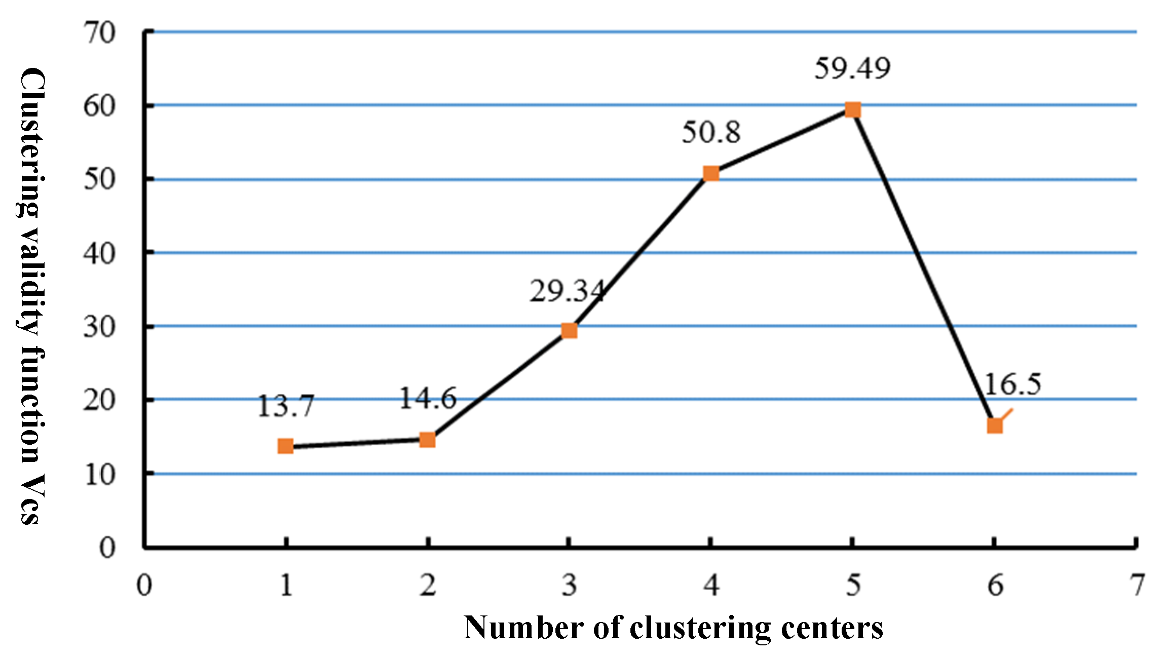
3.1.1. K-Means Clustering
3.1.2. FCM Algorithm
3.1.3. Frequency Ratio
3.2. Modeling Landslide Susceptibility
3.2.1. LR Model
3.2.2. RF
3.2.3. GBDT
3.2.4. AdaBoost-DT
3.2.5. Gini Index
3.2.6. Stacking
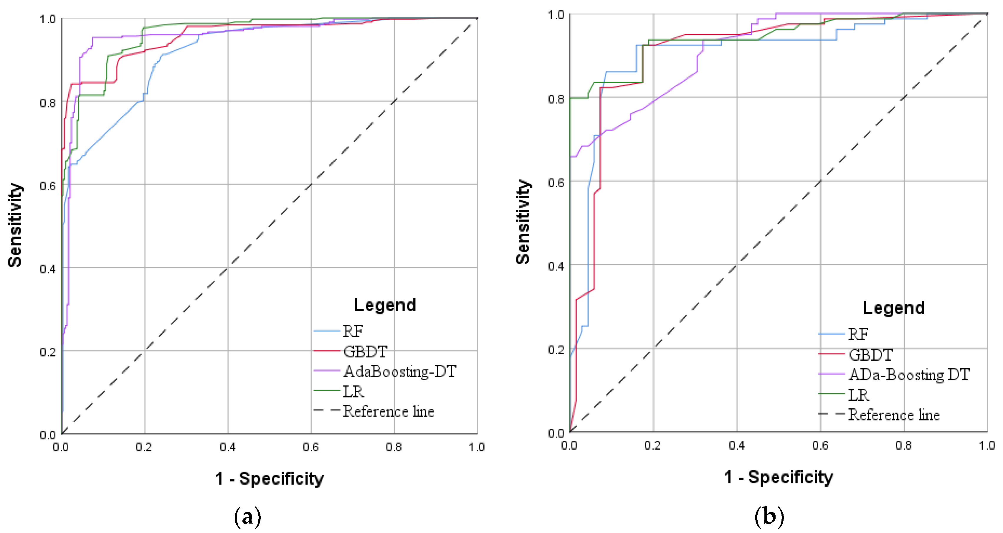
3.3. Evaluating Model Performance
4. Results and Verification
4.1. Non-Landslide Samples Selected by FCM and K-Means
4.2. Evaluation and Comparison of Different Models
4.3. Application of Stacking Method for LSM
4.4. Analysis of Major Conditioning Factors
5. Discussion
5.1. Ensuring the Reliability of Models
5.1.1. Internal and External Cross-Validation
5.1.2. The Selection of Non-Landslide Samples
5.2. Increasing the Accuracy of LSM
5.3. Maintain the Integrity of Geological Hazard Assessment
6. Conclusions
- The performance of different ensemble techniques varies, but achieved satisfactory results as a whole. Stacking was considered the most suitable model with obvious improvement in terms of accuracy compared to the basic classifiers.
- The combination of the bivariate statistical method and Gini index helps better explore the major conditioning factors and improve the integrity of ensemble techniques.
- The non-landslide samples selected by FCM are more representative and improved the quality of samples. Overall, improvement of sample quality and selection of advanced methods help improve the practicability of LSM.
Author Contributions
Funding
Institutional Review Board Statement
Informed Consent Statement
Data Availability Statement
Acknowledgments
Conflicts of Interest
References
- Huang, X.; Guo, F.; Deng, M.; Yi, W.; Huang, H. Understanding the deformation mechanism and threshold reservoir level of the floating weight-reducing landslide in the Three Gorges Reservoir Area, China. Landslides 2020, 17, 2879–2894. [Google Scholar] [CrossRef]
- Sun, X.; Chen, J.; Li, Y.; Rene, N.N. Landslide Susceptibility mapping along a rapidly uplifting river valley of the Upper Jinsha River, Southeastern Tibetan Plateau, China. Remote Sens. 2022, 14, 1730. [Google Scholar] [CrossRef]
- Kim, J.C.; Lee, S.; Jung, H.S.; Lee, S. Landslide susceptibility mapping using random forest and boosted tree models in Pyeong-Chang, Korea. Geocarto Int. 2018, 33, 1000–1015. [Google Scholar] [CrossRef]
- Safran, E.B.; O’Connor, J.E.; Ely, L.L.; House, P.K.; Grant, G.; Harrity, K.; Jones, E. Plugs or flood-makers? The unstable landslide dams of eastern Oregon. Geomorphology 2015, 248, 237–251. [Google Scholar] [CrossRef] [Green Version]
- Zhu, A.X.; Miao, Y.; Wang, R.; Zhu, T.; Deng, Y.; Liu, J.; Hong, H. A comparative study of an expert knowledge-based model and two data-driven models for landslide susceptibility mapping. Catena 2018, 166, 317–327. [Google Scholar] [CrossRef]
- Ayalew, L.; Yamagishi, H. The application of GIS-based logistic regression for landslide susceptibility mapping in the Kaku-da-Yahiko Mountains, Central Japan. Geomorphology 2005, 65, 15–31. [Google Scholar] [CrossRef]
- Jiao, Y.; Zhao, D.; Ding, Y.; Liu, Y.; Xu, Q.; Qiu, Y.; Liu, C.; Liu, Z.; Zha, Z.; Li, R. Performance evaluation for four GIS-based models purposed to predict and map landslide susceptibility: A case study at a World Heritage site in Southwest China. Catena 2019, 183, 104221. [Google Scholar] [CrossRef]
- Shi, M.; Chen, J.; Song, Y.; Zhang, W.; Song, S.; Zhang, X. Assessing debris flow susceptibility in Heshigten Banner, Inner Mongolia, China, using principal component analysis and an improved fuzzy C-means algorithm. Bull. Eng. Geol. Environ. 2016, 75, 909–922. [Google Scholar] [CrossRef]
- Liang, Z.; Wang, C.M.; Zhang, Z.M.; Khan, K.U.J. A comparison of statistical and machine learning methods for debris flow susceptibility mapping. Stoch. Environ. Res. Risk Assess. 2020, 34, 1887–1907. [Google Scholar] [CrossRef]
- Lian, C.; Zeng, Z.; Yao, W.; Tang, H. Extreme learning machine for the displacement prediction of landslide under rainfall and reservoir level. Stoch. Environ. Res. Risk Assess. 2014, 28, 1957–1972. [Google Scholar] [CrossRef]
- Merghadi, A.; Abderrahmane, B.; Tien Bui, D. Landslide susceptibility assessment at Mila Basin (Algeria): A comparative as-sessment of prediction capability of advanced machine learning methods. ISPRS Int. J. Geo-Inf. 2018, 7, 268. [Google Scholar] [CrossRef] [Green Version]
- Tien Bui, D.; Ho, T.C.; Revhaug, I.; Pradhan, B.; Nguyen, D.B. Landslide Susceptibility Mapping Along the National Road 32 of Vietnam Using GIS-Based J48 Decision Tree Classifier and Its Ensembles[M]//Cartography from Pole to Pole; Springer: Berlin/Heidelberg, Germany, 2014; pp. 303–317. [Google Scholar]
- Hu, X.; Zhang, H.; Mei, H.; Xiao, D.; Li, Y.; Li, M. Landslide susceptibility mapping using the stacking ensemble machine learning method in Lushui, Southwest China. Appl. Sci. 2020, 10, 4016. [Google Scholar] [CrossRef]
- Bennett, G.L.; Miller, S.R.; Roering, J.J.; Schmidt, D.A. Landslides, threshold slopes, and the survival of relict terrain in the wake of the Mendocino Triple Junction. Geology 2016, 44, 363–366. [Google Scholar] [CrossRef] [Green Version]
- Du, J.; Glade, T.; Woldai, T.; Chai, B.; Zeng, B. Landslide susceptibility assessment based on an incomplete landslide in-ventory in the Jilong Valley, Tibet, Chinese Himalayas. Eng. Geol. 2020, 270, 105572. [Google Scholar] [CrossRef]
- Lee, S.; Min, K. Statistical analysis of landslide susceptibility at Yongin, Korea. Environ. Earth Sci. 2001, 40, 1095–1113. [Google Scholar] [CrossRef]
- Breiman, L. Random forests. Mach. Learn. 2001, 45, 5–32. [Google Scholar] [CrossRef] [Green Version]
- Varnes, D.J. Landslide types and processes. Landslides Eng. Pract. 1958, 24, 20–47. [Google Scholar]
- Furlani, S.; Ninfo, A. Is the present the key to the future? Earth-Sci. Rev. 2015, 142, 38–46. [Google Scholar] [CrossRef]
- Guzzetti, F.; Galli, M.; Reichenbach, P.; Ardizzone, F.; Cardinali, M.; Galli, M. Estimating the quality of landslide susceptibility models. Geomorphology 2006, 81, 166–184. [Google Scholar] [CrossRef]
- Guzzetti, F.; Galli, M.; Reichenbach, P.; Ardizzone, F.; Cardinali, M. Landslide hazard assessment in the Collazzone area, Umbria, Central Italy. Nat. Hazards Earth Syst. Sci. 2006, 6, 115–131. [Google Scholar] [CrossRef]
- Sun, X.L.; Zhao, Y.G.; Wang, H.L.; Yang, L.; Qin, C.Z.; Zhu, A.X.; Li, B. Sensitivity of digital soil maps based on FCM to the fuzzy exponent and the number of clusters. Geoderma 2012, 171, 24–34. [Google Scholar] [CrossRef]
- Van Westen, C.J.; Castellanos, E.; Kuriakose, S.L. Spatial data for landslide susceptibility, hazard, and vulnerability assessment: An overview. Eng. Geol. 2008, 102, 112–131. [Google Scholar] [CrossRef]
- Feizizadeh, B.; Blaschke, T.; Nazmfar, H. GIS-based ordered weighted averaging and dempster—Shafer methods for landslide susceptibility mapping in the Urmia Lake Basin, Iran. Int. J. Digit. Earth 2012, 7, 688–708. [Google Scholar] [CrossRef]
- Hong, H.; Pradhan, B.; Xu, C.; Bui, D.T. Spatial prediction of landslide hazard at the Yihuang area (China) using two-class kernel logistic regression, alternating decision tree and support vector machines. Catena 2015, 133, 266–281. [Google Scholar] [CrossRef]
- Magliulo, P.; Di Lisio, A.; Russo, F.; Zelano, A. Geomorphology and landslide susceptibility assessment using GIS and bivariate statistics: A case study in southern Italy. Nat. Hazards 2008, 47, 411–435. [Google Scholar] [CrossRef]
- Liang, Z.; Wang, C.; Han, S.; Khan, K.U.J.; Liu, Y. Classification and susceptibility assessment of debris flow based on a semi-quantitative method combination of the fuzzy C-means algorithm, factor analysis and efficacy coefficient. Nat. Hazards Earth Syst. Sci. 2020, 20, 1287–1304. [Google Scholar] [CrossRef]
- Evans, I.S. An integrated system of terrain analysis and slope mapping. Z. Geomorphol. 1980, 36, 274–295. [Google Scholar]
- Camilo, D.C.; Lombardo, L.; Mai, P.M.; Dou, J.; Huser, R. Handling high predictor dimensionality in slope-unit-based landslide susceptibility models through LASSO-penalized generalized linear model. Environ. Model. Softw. 2017, 97, 145–156. [Google Scholar] [CrossRef] [Green Version]
- Dou, J.; Yamagishi, H.; Xu, Y.; Zhu, Z.; Yunus, A.P. Characteristics of the Torrential Rainfall-Induced Shallow Landslides by Typhoon Bilis, in July 2006, Using Remote Sensing and GIS[M]//GIS Landslide; Springer: Tokyo, Japan, 2017; pp. 221–230. [Google Scholar]
- Anil, K. Data clustering: 50 years beyond K-Means. Pattern Recogn. Lett. 2010, 31, 651–666. [Google Scholar]
- Hartigan, J.; Wong, M. Algorithm AS 136: A K-means clustering algorithm. J. R. Stat. Soc. C. 1979, 28, 100–108. [Google Scholar] [CrossRef]
- Dunn, J.C. A fuzzy relative of the ISODATA process and its use in detecting compact well-separated clusters. J. Cybern. 1973, 3, 32–57. [Google Scholar] [CrossRef]
- Bezdek, J.C. Pattern Recognition with Fuzzy Objective Function Algorithms; Springer Science & Business Media: Berlin/Heidelberg, Germany, 2013. [Google Scholar]
- Wang, J.; Chen, J.; Yang, J. Application of distance discriminant analysis method in classification of surrounding rock mass in highway tunnel. J. Jilin Univ. 2008, 38, 999–1004. [Google Scholar]
- Chen, J.; Pi, D. A cluster validity index for fuzzy clustering based on non-distance. In Proceedings of the 2013 International Conference on Computational and Information Sciences, Yongzhou, China, 21–23 June 2013; pp. 880–883. [Google Scholar]
- Neter, J.; Wasserman, W.; Kutner, M.H. Applied Linear Statistical Models; Irwin: Chicago, IL, USA, 1996. [Google Scholar]
- Fernández-Delgado, M.; Cernadas, E.; Barro, S.; Amorim, D. Do we need hundreds of classifiers to solve real world classification problems? J. Mach. Learn. Res. 2014, 15, 3133–3181. [Google Scholar]
- Pedregosa, F.; Varoquaux, G.; Gramfort, A.; Michel, V.; Thirion, B.; Grisel, O.; Blondel, M.; Prettenhofer, P.; Weiss, R.; Dubourg, V.; et al. Scikit-learn: Machine learning in Python. J. Mach. Learn. Res. 2011, 12, 2825–2830. [Google Scholar]
- Youssef, A.M.; Pradhan, B.; Jebur, M.N.; El-Harbi, H.M. Landslide susceptibility mapping using ensemble bivariate and multivariate statistical models in Fayfa area, Saudi Arabia. Environ. Earth Sci. 2014, 73, 3745–3761. [Google Scholar] [CrossRef]
- Wang, Y.; Feng, L.; Li, S.; Ren, F.; Du, Q. A hybrid model considering spatial heterogeneity for landslide susceptibility mapping in Zhejiang Province, China. Catena 2020, 188, 104425. [Google Scholar] [CrossRef]
- Freund, Y.; Schapire, R.E. A decision-theoretic generalization of online learning and an application to boosting. J. Comput. Syst. Sci. 1997, 55, 119–139. [Google Scholar] [CrossRef] [Green Version]
- Džeroski, S.; Ženko, B. Is combining classifiers with stacking better than selecting the best one? Mach. Learn. 2004, 54, 255–273. [Google Scholar] [CrossRef] [Green Version]
- Chung, C.J.F.; Fabbri, A.G. Validation of spatial prediction models for landslide hazard mapping. Nat. Hazards 2003, 30, 451–472. [Google Scholar] [CrossRef]
- James, G.; Witten, D.; Hastie, T.; Tibshirani, R. An Introduction to Statistical Learning; Springer: New York, NY, USA, 2013. [Google Scholar]
- Green, D.M.; Swets, J.A. Signal Detection Theory and Psychophysics; Wiley: New York, NY, USA, 1966. [Google Scholar]
- Schratz, P.; Muenchow, J.; Iturritxa, E.; Richter, J.; Brenning, A. Hyperparameter tuning and performance assessment of statistical and machine-learning algorithms using spatial data. Ecol. Model. 2019, 406, 109–120. [Google Scholar] [CrossRef] [Green Version]
- Duarte, E.; Wainer, J. Empirical comparison of cross-validation and internal metrics for tuning SVM hyperparameters. Pattern Recognit. Lett. 2017, 88, 6–11. [Google Scholar] [CrossRef]
- Bengio, Y. Gradient-based optimization of hyperparameters. Neural Comput. 2000, 12, 1889–1900. [Google Scholar] [CrossRef] [PubMed]
- Reichenbach, P.; Rossi, M.; Malamud, B.D.; Mihir, M.; Guzzetti, F. A review of statistically-based landslide susceptibility models. Earth-Sci. Rev. 2018, 180, 60–91. [Google Scholar] [CrossRef]
- Ciurleo, M.; Cascini, L.; Calvello, M. A comparison of statistical and deterministic methods for shallow landslide susceptibility zoning in clayey soils. Eng. Geol. 2017, 223, 71–81. [Google Scholar] [CrossRef]
- Liu, R.; Yang, X.; Xu, C.; Wei, L.; Zeng, X. Comparative study of convolutional neural network and conventional machine learning methods for landslide susceptibility mapping. Remote Sens. 2022, 14, 321. [Google Scholar] [CrossRef]
- Dou, J.; Yunus, A.P.; Bui, D.T.; Merghadi, A.; Sahana, M.; Zhu, Z.; Chen, C.; Han, Z.; Pham, B.T. Improved landslide assessment using support vector machine with bagging, boosting, and stacking ensemble machine learning framework in a mountainous watershed, Japan. Landslides 2020, 17, 641–658. [Google Scholar] [CrossRef]
- Di Napoli, M.; Carotenuto, F.; Cevasco, A.; Confuorto, P.; Di Martire, D.; Firpo, M.; Pepe, G.; Raso, E.; Calcaterra, D. Machine learning ensemble modelling as a tool to improve landslide susceptibility mapping reliability. Landslides 2020, 17, 1897–1914. [Google Scholar] [CrossRef]
- Arabameri, A.; Chandra Pal, S.; Rezaie, F.; Chakrabortty, R.; Saha, A.; Blaschke, T.; Thi Ngo, P.T. Decision tree based ensemble machine learning approaches for landslide susceptibility mapping. Geocarto Int. 2021, 1–35. [Google Scholar] [CrossRef]
- Li, W.; Fang, Z.; Wang, Y. Stacking ensemble of deep learning methods for landslide susceptibility mapping in the Three Gorges Reservoir area. China. Stoch. Environ. Res. Risk Assess. 2021, 1–22. [Google Scholar] [CrossRef]
- Chen, W.; Xie, X.; Wang, J.; Pradhan, B.; Hong, H.; Bui, D.T.; Ma, J. A comparative study of logistic model tree, random forest, and classification and regression tree models for spatial prediction of landslide susceptibility. Catena 2017, 151, 147–160. [Google Scholar] [CrossRef] [Green Version]
- Dietterich, T.G. An experimental comparison of three methods for constructing ensembles of decision trees: Bagging, boosting, and randomization. Mach. Learn. 2000, 40, 139–157. [Google Scholar] [CrossRef]
- Youssef, A.M.; Pourghasemi, H.R. Landslide susceptibility mapping using machine learning algorithms and comparison of their performance at Abha Basin, Asir Region, Saudi Arabia. Geosci. Front. 2021, 12, 639–655. [Google Scholar] [CrossRef]


| Category | Conditioning Factors | Type | Data Source | Values |
|---|---|---|---|---|
| Topographical | Elevation (m) | Continuous | SRTM | (1) <200; (2) 200–400; (3) 400–600; (4) 600–800; |
| (5) >800 | ||||
| Plan curvature | Continuous | SRTM | (1) <0; (2) 0–0.01; (3) 0.01–0.02; (4) 0.02–0.03; | |
| (5) >0.03 | ||||
| Profile curvature | Continuous | SRTM | (1) <0; (2) 0–0.01; (3) 0.01–0.02; (4) 0.02–0.03; | |
| (5) >0.03 | ||||
| Slope angle (°) | Continuous | SRTM | (1) <10; (2) 10–20; (3) 20–30; (4) >30 | |
| TWI | Continuous | SRTM | (1) <6.5; (2) 6.5–7; (3) 7–7.5; (4) 7.5–8; | |
| (5) 8–8.5; (6) >8.5 | ||||
| MED (m) | Continuous | SRTM | (1) <100; (2) 100–200; (3)200–300; (4) 300–400; | |
| (5) 400–500; (6) >500 | ||||
| Slope aspect | Categorical | SRTM | (1) north; (2) northeast; (3) east; (4) southeast; (5) south; (6) southwest; (7) west; (8) northwest | |
| Geological and Geomorphological | Distance to faults (m) | Continuous | Geological map | (1) <1000; (2) 1000–2000; (3) 2000–3000; (4)3000–4000; (5) >4000 |
| Distance to streams (m) | Continuous | DNRB | (1) <1000; (2) 1000–2000; (3) 2000–3000; (4)3000–4000; (5) >4000 | |
| Lithology | Categorical | Geological map | (1) Gneiss; (2) Dolomites; (3) Siltstone (4) Granite;(5) Limestone; (6) Conglomerate | |
| Triggering factors | Maximum 24 h rainfall (mm) | Continuous | BHM | (1) <270; (2) 270–280; (3) 280–290; (4) >290 |
| Maximum 7 days rainfall (mm) | Continuous | BHM | (1) <320; (2) 320–330; (3) 330–340; (4) >340 | |
| Distance to roads (m) | Continuous | DNRB | (1) <1000; (2) 1000–2000; (3) 2000–3000; (4)3000–4000; (5) >4000 |
| Methods | Parameters |
|---|---|
| DT | Criterion = ‘gini’; max_features = None; max_depth = 20; min_samples_split = 2; min_samples_leaf = 1; max_leaf_nodes = None; class_weight = None |
| RF | n_estimators = 500; criterion = ‘gini’; max_depth = None; max_features = ‘sqrt’; |
| GBDT | n_estimators = 100; learning_rate = 0.1; max_depth = 2; verbose = 1; subsample = 0.7; max_leaf_nodes = None |
| AdaBoost-DT | base_estimator = None; n_estimators = 100; learning_rate = 1.0; algorithm = ‘SAMME.R’; random_state = None |
| Method | Class | Landslide Ratio (%) | Area Ratio (%) | FR |
|---|---|---|---|---|
| FCM | Very low | 3.24 | 15.97 | 0.20 |
| Low | 19.73 | 23.25 | 0.85 | |
| Moderate | 21.35 | 19.29 | 1.11 | |
| High | 40.00 | 33.50 | 1.19 | |
| Very high | 15.68 | 8.00 | 1.96 | |
| k-means | Very low | 1.62 | 11.66 | 0.14 |
| Low | 15.41 | 22.30 | 0.69 | |
| Moderate | 15.57 | 18.71 | 0.83 | |
| High | 48.11 | 39.16 | 1.22 | |
| Very high | 17.30 | 8.17 | 2.11 |
| Metrics | RF | GBDT | Ada-DT | Stacking |
|---|---|---|---|---|
| TP (%) | 82.46 | 84.88 | 81.29 | 91.22 |
| TN (%) | 76.80 | 87.67 | 86.44 | 92.20 |
| FP (%) | 17.54 | 15.12 | 18.71 | 8.78 |
| FN (%) | 23.2 | 12.37 | 13.56 | 7.80 |
| Sensitivity (%) | 79.93 | 86.97 | 85.66 | 91.89 |
| Specificity (%) | 83.16 | 85.67 | 82.26 | 91.78 |
| Accuracy (%) | 81.56 | 86.29 | 83.87 | 91.84 |
| Models | AUC | Standard Error | 95% Confidence Interval |
|---|---|---|---|
| RF | 0.920 | 0.011 | 0.899–0.941 |
| GBDT | 0.957 | 0.008 | 0.942–0.973 |
| Ada-DT | 0.959 | 0.009 | 0.942–0.976 |
| Stacking | 0.963 | 0.006 | 0.950–0.975 |
| Metrics | RF | GBDT | Ada-DT | Stacking |
|---|---|---|---|---|
| TP (%) | 77.22 | 86.30 | 83.54 | 90.54 |
| TN (%) | 79.71 | 83.78 | 86.96 | 91.78 |
| FP (%) | 22.78 | 13.70 | 16.46 | 9.46 |
| FN (%) | 20.29 | 16.22 | 13.04 | 8.22 |
| Sensitivity (%) | 81.33 | 86.11 | 86.96 | 91.78 |
| Specificity (%) | 75.34 | 84.00 | 82.19 | 90.54 |
| Accuracy (%) | 78.38 | 85.03 | 85.13 | 91.16 |
| Models | AUC | Standard Error | 95% Confidence Interval |
|---|---|---|---|
| RF | 0.906 | 0.027 | 0.853–0.959 |
| GBDT | 0.910 | 0.026 | 0.859–0.962 |
| Ada-DT | 0.917 | 0.021 | 0.877–0.958 |
| Stacking | 0.944 | 0.018 | 0.908–0.980 |
| Method | DTS | DTR | Elevation | Slope Angel | TWI | Maximum 24 h Rainfall | Lithology | MED | Maximum 7 Days Rainfall | Profile Curvature |
|---|---|---|---|---|---|---|---|---|---|---|
| GBDT | 0.37 | 0.34 | 0.16 | 0.04 | 0.03 | 0.02 | 0.01 | 0.01 | 0.01 | 0.01 |
| Conditioning Factor | Zone | Landslide (%) | Non-Landslide (%) | FR |
|---|---|---|---|---|
| DTS(m) | <1000 | 46.99% | 0.95% | 49.30 |
| 1000–2000 | 24.43% | 0.14% | 173.29 | |
| 2000–3000 | 14.33% | 6.63% | 2.16 | |
| 3000–4000 | 5.33% | 15.72% | 0.34 | |
| >4000 | 8.91% | 76.69% | 0.12 | |
| DTR(m) | <1000 | 56.06% | 7.13% | 7.87 |
| 1000–2000 | 23.02% | 7.13% | 3.23 | |
| 2000–3000 | 15.59% | 9.29% | 1.68 | |
| 3000–4000 | 3.95% | 11.51% | 0.34 | |
| >4000 | 1.37% | 66.79% | 0.02 | |
| Elevation(m) | <200 | 4.36% | 2.08% | 2.09 |
| 200–400 | 53.76% | 12.29% | 4.37 | |
| 300–600 | 30.36% | 23.70% | 1.28 | |
| 400–800 | 10.06% | 34.52% | 0.29 | |
| >800 | 1.46% | 27.41% | 0.05 |
Publisher’s Note: MDPI stays neutral with regard to jurisdictional claims in published maps and institutional affiliations. |
© 2022 by the authors. Licensee MDPI, Basel, Switzerland. This article is an open access article distributed under the terms and conditions of the Creative Commons Attribution (CC BY) license (https://creativecommons.org/licenses/by/4.0/).
Share and Cite
Liang, Z.; Liu, W.; Peng, W.; Chen, L.; Wang, C. Improved Shallow Landslide Susceptibility Prediction Based on Statistics and Ensemble Learning. Sustainability 2022, 14, 6110. https://doi.org/10.3390/su14106110
Liang Z, Liu W, Peng W, Chen L, Wang C. Improved Shallow Landslide Susceptibility Prediction Based on Statistics and Ensemble Learning. Sustainability. 2022; 14(10):6110. https://doi.org/10.3390/su14106110
Chicago/Turabian StyleLiang, Zhu, Wei Liu, Weiping Peng, Lingwei Chen, and Changming Wang. 2022. "Improved Shallow Landslide Susceptibility Prediction Based on Statistics and Ensemble Learning" Sustainability 14, no. 10: 6110. https://doi.org/10.3390/su14106110