On the Issues of Spatial Modeling of Non-Standard Profiles by the Example of Electromagnetic Emission Measurement Data

Abstract

This paper examines the possibility of the spatial modelling of the Earth’s natural pulsed-electromagnetic-field measured values, which form a closed profile without the data inside. This geophysical method allows us to map active tectonic movement which breaches the integrity of pipes. During the experiment, 4.5 km of profiles were measured in the Admiralteysky district of St. Petersburg, Russia. Regular electromotive force (EMF) values and anomalous EMF values were obtained, ranging from 0 to 900 µV and above 900 µV, respectively. The anomalous values are associated with tectonic faults in the bedrock. The data obtained are characterized by complex spatial anisotropy associated with the development of two groups of tectonic faults of different orientations. The authors have considered the problems of the spatial modeling of the data obtained. The main problems, the solutions to which should allow the obtaining of adequate models, have been identified. Based on the analysis of the measurement results, geological features of the studied areas, as well as variography, the following possible solutions were proposed: changing the measurement technique; dividing the data array according to the main directions of anisotropy; the need to introduce additional correction coefficients. The problem revealed in this article requires further research on the basis of the obtained results, which will reduce the cost and timing of such studies, and, as a result, give an opportunity to take into account active tectonic disturbances during the construction and scheduled maintenance of underground utilities, which is especially important within the framework of the concept of sustainable development.

1. Introduction

Ensuring the safety of human life in the urban environment, as well as limiting the negative impact of economic activities on the environment, is an integral part of the concept of the sustainable development of territories [1,2]. Close attention is also paid to the planning of residential areas and related engineering infrastructure—road junctions, electrical and heating networks [3], water supply and drainage systems, sewerage, etc.—as well as the improvement of territories [4] and the creation of social infrastructure [5,6]. These are extremely important and, beyond any doubt, relevant issues. However, in addition to creating new infrastructure, there is a need to optimally integrate existing infrastructures, subjected to rationalization, into this concept [7,8].

Water supply and drainage systems, as well as heating networks in many cities, were built a long time ago and without proper consideration of geological conditions [9,10]. However, geology has a significant impact on the integrity of linear objects due to the intensification of movement along tectonic faults [11], the influence of microbiota in fault zones [12], and erosive processes [13]. If, in new districts, these conditions can be accounted for during construction, in old districts, it seems optimal to partially change the structures by strengthening the sections crossing the fault. Regardless of further technological measures, taking into account active tectonic faults will potentially reduce the scope of repair work and potential adverse effects from pipeline ruptures.

In mining, when designing mine workings, and gas storage collectors, as well as at other special hazardous facilities, in particular those related to the nuclear power industry, tectonic faults and their intersection nodes have long been taken into account as areas of the most probable occurrence of dynamic phenomena and destruction of the massif (collapses, falls, rock bumps, etc.) [14,15,16,17,18,19]. The preliminary geodynamic zoning of territories is carried out for these objects [20].

Geodynamic zoning is a method for studying the block structure and the stress state of a rock mass, and identifying, assessing, and controlling currently active structures, such as active faults, geodynamic zones, and associated risk zones, in order to improve the geodynamic and environmental safety of industrial and civil objects during the development of subsoil and the Earth’s surface.

For objects located at great depths, this work is mandatory, but for shallow-buried objects the performance of such work may also be expedient, especially when considering this issue in terms of sustainable development.

Previously, the authors have already compared data on accidents involving underground utilities and information on the position of known tectonic faults. This work made it possible to conclude that there is a high convergence of potentially geodynamically dangerous areas and areas of accidents [11]. In that study, the data were represented in graphs with characteristic features of the profile (electromagnetic (EM) sources, faults, georeferencing, etc.) plotted along the abscissa axis. However, this method does not make it possible to fully assess the nature of the distribution of values over the area, the presence of patterns, local anomalies that have no geological explanation, etc.

A logical continuation of the work already done is a systematization of the accumulated data on measurements of the Earth’s natural pulsed electromagnetic field (ENPEMF) and geological data available from open sources, as well as their convenient and informative visualization. Integration of these data into the model will make their accounting, when planning and re-constructing urban infrastructure, simple and understandable even for those not proficient in this field.

St. Petersburg (59°57′00″ north latitude, 30°19′00″ east longitude), which in previous works has already served as an experimental area for studies, is well suited for a continuation thereof [11]. The geology of the city has been well studied to great depths, due to the deep burial of tunnels and subway lobbies (about 100 m) and high complexity of construction due to the features of the soil, characterized by significant heterogeneity and the development of swamps [21,22]. The geology of the city will be more thoroughly described in Section 2.1.

Studies of various scientific schools are devoted to the construction of maps based on the ENPEMF parameters. For example, in [23], based on the construction of maps of the electromagnetic field flux density, it is recommended to lay a pipeline, as well as to arrange drainage wells in places with minimum values of the electromagnetic field density. However, the paper does not disclose the method of map construction; therefore, it is difficult to determine its accuracy. In the study of [24], natural neighbor interpolation and inverse distance weight (Kriging) methods are used to estimate the electromagnetic field levels that workers are exposed to in the supply chain of an air-insulated substation. However, just like in the previous work, the data set is a regular grid of measurements. The paper [25] presents the results of magnetotelluric and electromagnetic time-domain soundings on the basis of which a geoelectric model was built, which makes it possible to determine the architectural geometry of the geological environment and variations in the physical properties of various blocks of the Earth’s crust limited by large electrical inhomogeneities. Thus, this work also confirms the relationship between the parameters of the electromagnetic field and tectonic disturbances.

Various geostatistical methods are actively used to solve similar problems, in particular for modeling the spatial distribution of environmental data [26] and assessing the homogeneity of data [27]. These works, along with numerous other materials [28,29] containing examples of spatial modeling in geology, ecology, geophysics, etc., are a good basis for conducting this study. Nonetheless, they do not contain a solution to the main problem associated with modeling the data of measurements of the ENPEMF, which acts as a marker of active tectonic faults.

Nonetheless, in all works, the data array is represented either by a regular grid or by a random distribution of data over the entire study area. The task of constructing a spatial model in the conditions of a limited data set was not set. At the same time, it is worth noting that the anisotropy of the experimental data obtained in this study, on the one hand, is not spatially sustained, and, on the other hand, the territory could not be simply and unambiguously zoned due to the ubiquitous spread of the tectonics in three azimuthal directions. In addition, it was difficult to take measurements within the study area for three reasons: the dense and complex urban development of the city center, associated labor costs and time spending, as well as the research technique being based on profiling the area wherein tectonics are crossed with a dense line of measurements.

Thus, the aim of the study is to assess the possibility of constructing a spatial interpolation model in the conditions of random values of experimental data and the spatial distribution of data along the perimeter in the absence of values within the measured area. It should be noted that the authors of [30] claim that kriging is an effective way to estimate random fields with a local concentration. These are all prerequisites and possibilities to achieve the goal of choosing the methods of future interpolation and spatial visualization of the ENPEMF measurement data, but it is necessary to solve a number of related tasks. The main tasks include:

• Search for anisotropy of measurement data displaying tectonic faults.
• Determination of an effective way of displaying anisotropy when constructing a spatial interpolation model under experimental conditions.
• Assessment of the possibility of determining active tectonics during large-scale areal measurement of the ENPEMF parameters.

2. Materials and Methods

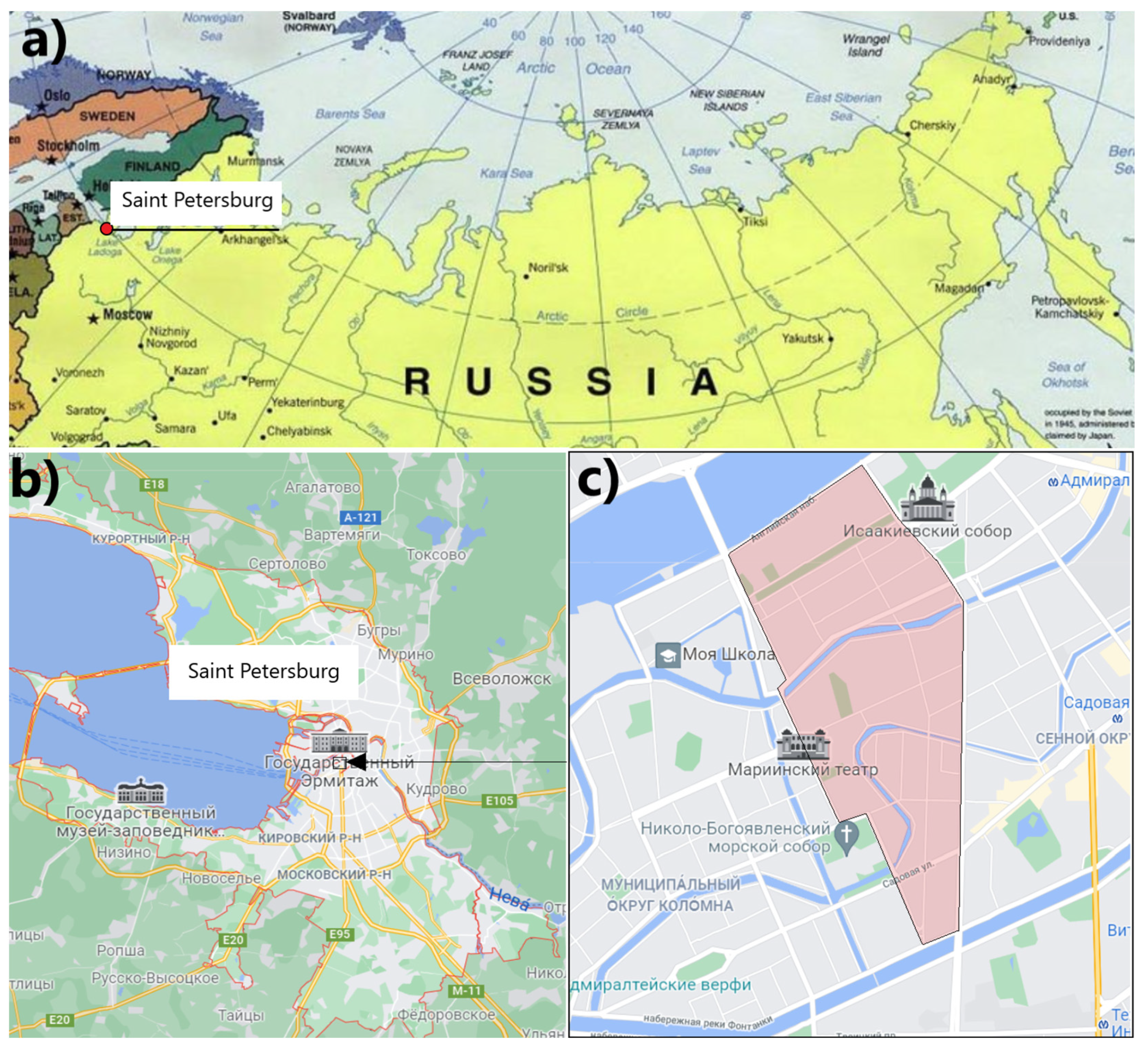
2.1. Study Area

A closed profile in the center of the city, in the Admiralteysky district (Figure 1), was chosen as the reference one. From the viewpoint of building system, this site is suitable, since there are no industrial facilities, and the height of the residential buildings is insignificant (from 3 to 5 floors) and consistent. From a geological point of view, it is interesting because it is crossed by six tectonic faults at once.

The main features of the selected profile will be presented further in Section 2.3.

St. Petersburg is located in the northwest of the Russian Plate, which is an area of the foundation immersed under the sedimentary cover [33]. The occurrence of rocks is monoclinal, with an orientation to the south. The changing of layers to younger ones can be observed in the same direction.

St. Petersburg is characterized by crystalline rocks of the Archean and Proterozoic groups, mainly represented by granites, gneisses, and diorites. Basement rocks, on average, occur at a depth of 180–240 m [34], while in the south the depth can reach up to 300 m.

Above, are the deposits of the Vendian system: the Redkinskiy and Kotlinskiy horizons. The Redkinskiy horizon is represented by sandstones and siltstones with a thickness of 10–30 m, as well as by claystone-like clays and siltstones with a thickness of at most 15 m. The Kotlin deposits in the lower sub-formation are represented by sandstones and siltstones, and, in the upper sub-formation, by clays with rare sandstone interlayers. The thickness of this layer in some places reaches 150 m, but the surface of the Vendian complex is strongly eroded and varies greatly [35].

Quaternary deposits overlap the territory throughout the city. Their average thickness varies from 20 to 30 m, but in places of buried river valleys it reaches 100–130 m. The sedimentary cover is characterized by frequent lithological variability but is mainly represented by weak sandy-clayey soils.

The profile of the city is shown in Figure 2.

Below, a brief stratigraphic characteristic of the rocks in the investigated part of the city (in Figure 2, the region in the area of the Neva River) is presented.

The electromagnetic properties of soils were given in previous studies, wherein it was found that the use of the ENPEMF registration method is suitable for these soils. The properties of rocks do not prevent the field from passing through the strata, and the depth of the studied sources, which are geodynamically active faults (GDAFs), is insignificant, which also cannot result in attenuation of the electromagnetic wave causing an anomalous value in the measurement zone [11]. From the viewpoint of the fundamental theory, the waveform of the electromagnetic pulse generated by GDAFs, its frequency, period, and other parameters typical for the electromagnetic wave, are studied by various scientific schools, whose representatives are Mulev, S.N. [36], Frid, V. [37], Simpson, F. [38], and Sabaka, T. J. [39]. However, it is worth noting that studies are most often carried out for a specific area with its own geological structure and electromagnetic properties of soils [40,41].

Drainage systems, the most vulnerable from the viewpoint of accidents, represent linear objects of urban communications, which are usually shallow buried (15–90 m [42], in quaternary deposits). The sewers are buried deeper—in the Upper Kotlin clays (in the southern part of the city, this depth corresponds to the Lower Cambrian clays).

From a tectonic point of view, St. Petersburg is situated at the junction of two large structures: the Baltic Shield and the northwestern part of the Russian Plate. In this area, movements of the foundation blocks were recorded even in the modern, quaternary period. In addition, it was found that basement faults are prolonged in sedimentary rocks—clays and sandstones—disintegrating them [34]. The Verkhnekotlinsky clays are also fractured, as evidenced by the data on subway tunnels. The city is characterized by fault tectonics of northeastern, northwestern and sublatitudinal strike. In addition, there are paleovalleys in the city.

Previously, scientists from the Mining University conducted an analysis of sections constructed during the engineering of a subway line, which resulted in a map of tectonic faults, shown in Figure 3 [43,44]. This map is the geological basis for research, as it contains the most recent and complete information among open sources.

For large cities it is not possible to cover the entire area with a dense line of measurements, especially at the initial stages of the study when it is fraught with errors in the choice of the measurement pitch, the length of profiles, as well as in the method of data processing. The above-mentioned reasons behind the inaccuracy of measurements are associated with the fact that, to date, not a single measurement technique exists for taking measurements by the method of electromagnetic emission.

The measurement pitch and the length of the profile in this study were theoretically determined in advance and will be addressed in greater detail in Section 2.3. This work is mostly focused on the method of data processing, as it is the most relevant issue. At the same time, the task of the adequate spatial visualization of data comes first, including the selection of interpolation tools and the way of presenting the results of the analysis. In addition, determining a method of spatial interpolation for constructing such a map will allow for the interpolation of unknown profiles in the future.

2.2. Substantiation of the Processes of Electromagnetic Field Change in Zones of Tectonically Active Faults

According to the research, a pulsed electromagnetic field, which is a superposition of fields of different natures and frequencies, is recorded on the Earth’s surface. As is known, the Earth’s natural electromagnetic field has a frequency of about 10 Hz and is a low-frequency field, while fields of different natures will have frequencies that fall not only within the low- and mid-frequency ranges [45].

The main, non-interconnected, reasons for these fields are:

• Mechanoelectric phenomena in rocks, which occur during elastic or plastic deformation and destruction (piezoelectric effect, electrification of cracks) [46]. Deforming forces, resulting in mechanoelectric phenomena, arise due to changes in mechanical and hydrogeological properties, the stress state of the rock mass, and soils, etc. It was found that GDAFs are sources of such mechanoelectric phenomena [47].
• Thermal processes that result in exoelectronic emission from minerals. This phenomenon is caused by the release of weakly bound water, giving rise to an increase in electrical conductivity and a decrease in the activation energy of current carriers, followed by an increase in the number of emitted electromagnetic pulses [48].
• Microseismic oscillations [49,50]. Microseismical vibrations are caused by seismotectonic processes—fluctuations in the surface hardness of the earth.
• Man-made load—cable and overhead transmission lines, transformer substations, subway lines, and electric transport. However, the operating frequency, typical for man-made load, as a rule, is 50 Hz [51]. It is worth noting that there are no subway lines or industrial buildings in the studied part of the city. Due to the fact that electric transport is widely used in the city, measurements were stopped when a trolleybus or tram passed, so the impact of man-made load was minimal.
• Pulse signals from remote sources [52,53,54]. The main reasons behind their occurrence are atmospheric phenomena, namely lightning discharges. As a rule, among the remote sources, atmospherics and whistling atmospherics are distinguished, which are characterized by an extremely low frequency starting from a fraction of Hertz [55].
• Ionospheric and induced currents in the Earth’s deep interior at a depth of 100–600 km [56].

Since the principle of superposition is valid for the electromagnetic field, it is logical to assume that the occurrence of a new process in rocks or a change in another (existing) process will result in a change in the resulting field. Therefore, in the place of measurement, to which any of the above-mentioned phenomena is confined, the parameters of the electromagnetic field will differ upward or downward.

This paper, as already mentioned, discusses geodynamically active faults. The physics of the formation of changes in the parameters of the electromagnetic field in the zone of tectonically active faults is explained by the fundamental laws of electromagnetism, as well as by the theory of static and dynamic magnetic fields.

Within the framework of this study, the method of electromagnetic emission (EME), which was developed in the middle of the 20th century, was applied. The essence of the method is to measure the parameters of the electromagnetic field, including the intensity of the electromagnetic field (the pulse repetition rate of the field), the dominant frequency, signal amplitude, energy, and spectral density [57]. In this work, the derivative of only one parameter, namely the signal amplitude, expressed in EMF, was fixed. This approach has proved its efficiency in previous long-term studies [11]. Over the course of fieldwork, direct measurements of the EMF induced in the receiving antenna (magnetic rod with a ferrite core), described in detail in [11], were made when it entered a pulsed electromagnetic field. In order to minimize the man-made load (electric transport, road works, construction works, etc.), measurements were made early in the morning.

GDAFs are sources of pulsed electromagnetic waves (as sources of mechanoelectric phenomena), which result in a change in the resulting electromagnetic field on the surface of the measurement zone. The specific features of the passage of an electromagnetic pulse in an elastic medium, which rocks belong to, are disclosed in [58,59]. For most media, which include sands, clays and loams, granite, concrete, and asphalt, with varying degrees of humidity (these media represent the rock mass between GDAF and the measurement profile), the propagation of electromagnetic pulses depends mainly on the dielectric constant of the medium, and, to the greatest extent, on its imaginary component and humidity [60]. With an increase in the dielectric constant of the medium, the speed of signal propagation decreases. The penetration depth of the signal depends inversely on the specific attenuation and humidity. To minimize the impact of additional water cut, the studies were conducted in dry weather. Since the soil in which the electromagnetic wave propagates has a nonzero conductivity, the wave will attenuate when passing through it. However, due to the facts that the frequencies of the pulses under consideration lie in the range of 1–18 kHz and the wavelengths are more than 100 m with attenuation taken into account, after passing through the surface layer, an electromagnetic pulse can be registered with a receiving antenna [11].

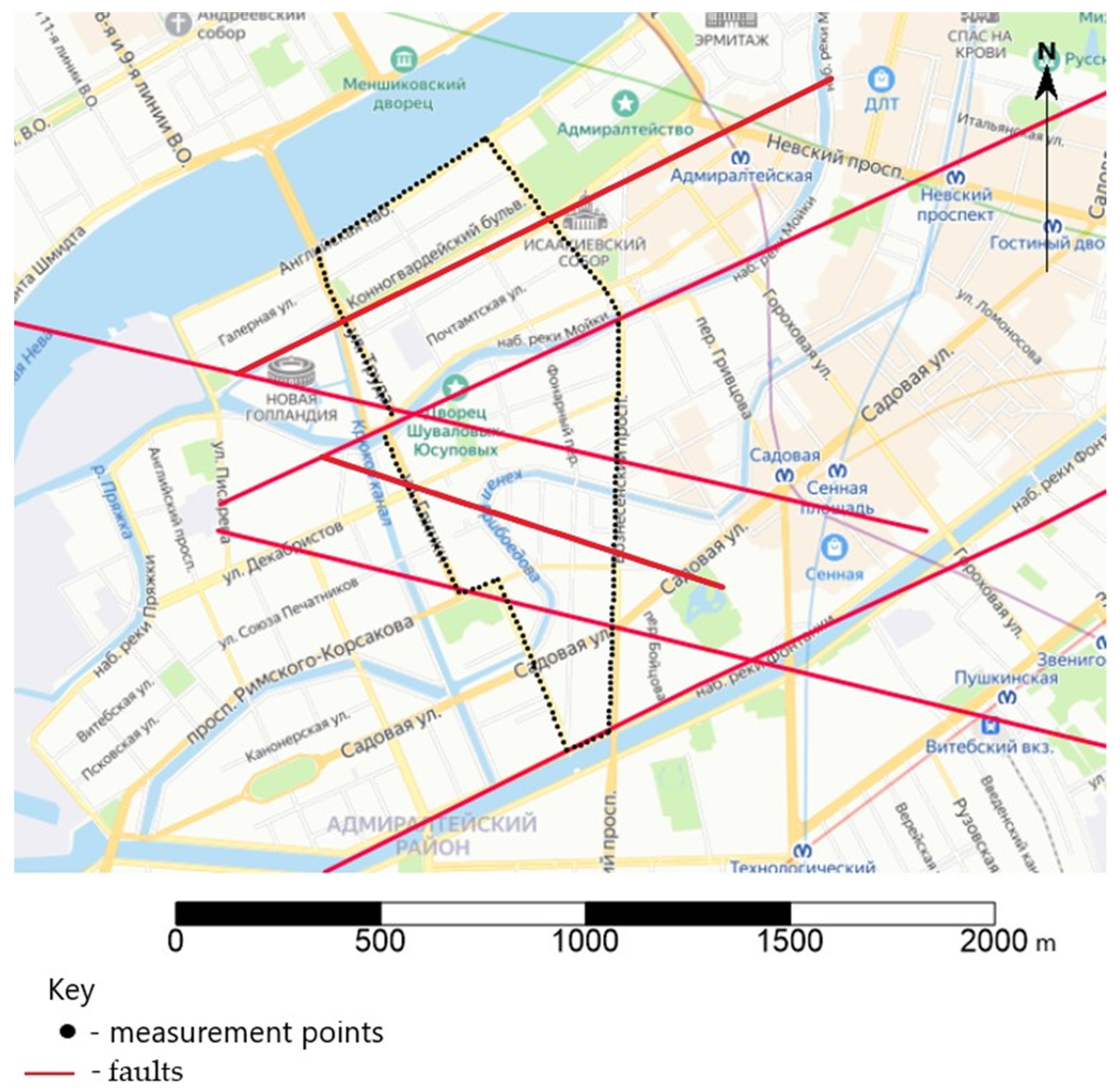
2.3. Monitoring Network

The studied profile was made earlier within the framework of the study on correlating the locations of active tectonic faults and accidents on pipelines [11], and the data showed high correspondence. In total, five closed profiles with a total length of more than 25 km were made (observing the average length of every single profile of about 5 km).

Table 1. Stratigraphy.

Stratigraphy		Depth, m	Rocks
Proterozoic acrothem Upper eonotema Vendian system Upper section Kotlinsky horizon—V2kt.	Lower Kotlinskaya subformation V2kt1	180–192	Alternating clays, sandstones, siltstones in the lower part of the section with a predominance of sandstones. The rocks are gray, greenish-gray, and brown.
	Upper Kotlinskaya subformation V2kt2	138–145	Alternating clays, sandstones, siltstones in the lower part of the section with a predominance of sandstones. Thin layering is characteristic.
Cenozoic eratema Quaternary system		Sediment thickness varies from 15–20 to 100–120 m	Versatile complex of different genetic types of sediments.

shows the measurement data of the ENPEMF magnetic characteristic, which were obtained in 2014. The statistical description of the spatial distribution [61,62] is used in this work due to the fact that the data obtained during the experiment have random distribution and do not allow obtaining a formulaic distribution law based on the physical processes that cause the phenomenon of EMF in the receiving antenna (see Section 2.1). In this study, the spatial variable is the magnitude of voltage U, recorded by the multimeter in the voltmeter mode (APPA-109N). The variable is measured in µV. This value is:

(1)

The data array comprises a set of 210 points;

(2)

It is a continuous variable;

(3)

It is spatially referenced;

(4)

It is spatially correlated.

Statistical parameters are presented in

Table 2. Simple statistics.

	Parameter	Value, µV
1	Mean, m	928.5
2	Median, M	630
3	Std. dev.	94.475
4	Min.	45
5	Per. 25	322.5
6	Per. 50	630
7	Per. 75	1100
8	Max.	6250

.

All profiles crossed tectonic faults with different strike azimuths. Thus, when processing every single street, no problems were encountered with regard to identifying anomalies and correlating them with tectonic faults or man-made sources. However, when trying to perform large-scale processing and modeling data of the ENPEMF measurements, there was a difficulty in interpolating data for different directions. The selected profile, due to the absence of intersections of tectonic faults of different strikes directly within the profile, allows convenient dividing of a common database into sub-bases without additional manipulations.

At the same time, as mentioned earlier, the task was no longer set to prove a correlation between the ENPEMF anomalies and the location of tectonic faults, since the existence of this correlation was confirmed over the previous years of research [11,60]. To further substantiate this relationship, it is also necessary to combine the already existing separate databases, increase the volume of measurements and correctly select interpolation methods that are characterized by the greatest efficiency in identifying tectonic faults.

Closed profiles allow the intersection of tectonic faults at two locations. Thus, there was no need to make additional profiles through the same tectonic faults that had already been crossed. The streets selected for profiling look optimal in terms of the ratio of labor costs and the amount of data received (Figure 4).

The study used the technique of discrete observations on the surface with a pitch of 20 m. With such a pitch, there will be at least 2 measurements in each zone of geodynamically active faults (GDAFs), the widths of which vary from 50 to 200 m. The total length of the profile was about 4.5 km.

The orientation of the magnetic moment of the antenna was chosen to be vertical. It is this direction of the antenna that has shown itself as the most efficient way in previous studies, and is also the only “geological” one, taking into account the slight slope feature in this part of the city.

The profile crosses several tectonic faults, which are grouped into two types: the upper part of the polygon is characterized by the development of tectonic faults of the northeastern strike, the lower part, by the northwestern one. Furthermore, in the lowest part of the polygon, at its southern end, the profile intersects and goes through 14 measurement points along a large tectonic fault of the northeastern strike. Thus, based on previous studies, two directions of anisotropy, typical for these measurements, should be expected.

In addition, this area is characterized by the following important geological features:

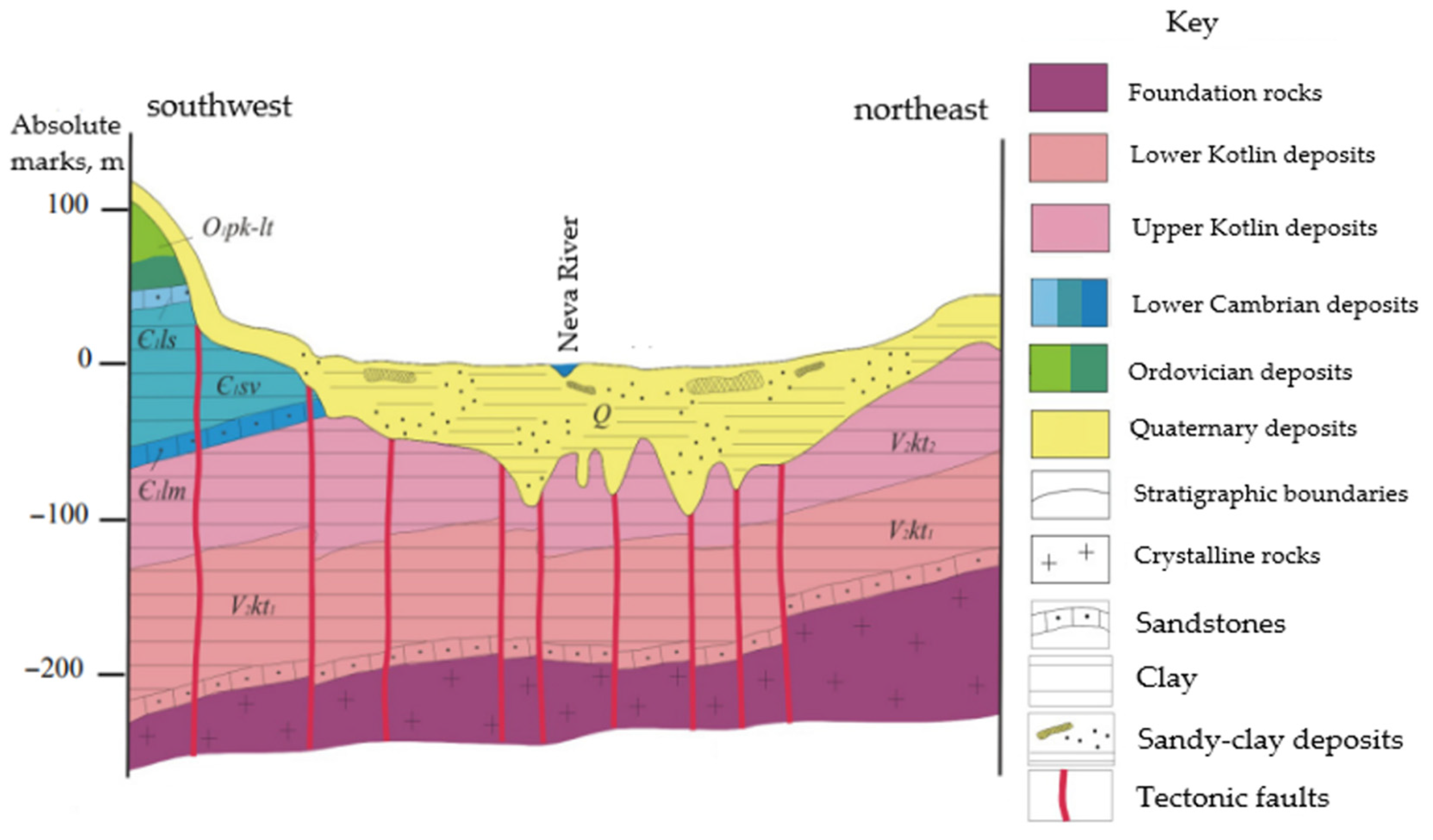
• The profile is not complicated by the presence of rock contacts, the intersection of which also causes changes in the structure of the ENPEMF [34];
• The profile partially crosses the ancient riverbeds [34], which makes it possible to analyze the impact of this factor on measurements;
• The thickness of quaternary deposits does not exceed 70 m [34].

Thus, taking into account the above-mentioned points and the general focus of the study, this profile makes it possible to analyze the possibilities of interpolation of the ENPEMF data by area and assess the prospects of visualization for the data type under consideration.

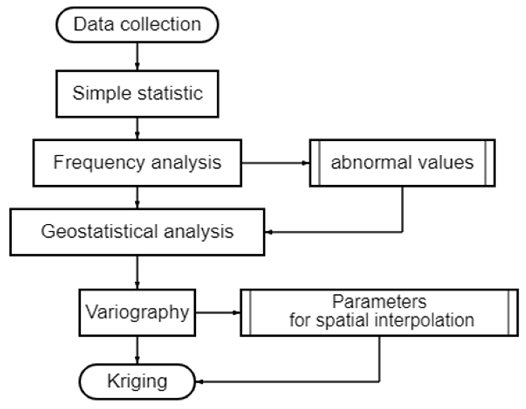
2.4. Applied Methods

In this work, methods of statistical and geostatistical analysis were used, including methods of spatial modeling. First of all, a statistical analysis of the measured data array was carried out. The following parameters were determined: average, maximum, and minimum values, and frequency distribution histograms were constructed. The abovementioned parameters were determined according to the classical theory of statistical analysis [63]. Construction of frequency distribution histograms is necessary to determine the anomalous values corresponding to active tectonic zones. The purpose of the geostatistical analysis was to obtain the parameters necessary for building a spatial model—the main and secondary directions of data correlation, and determining the maximum distances at which the correlation is maintained. The spatial model firstly should not overload the map with data, but, at the same time, it is necessary to provide all its users with sufficient information to make it feasible to reveal possible sources of anomalies. The kriging method was used to build the spatial model.

Kriging is one of the methods used to create grids in the Surfer 13 program [64], which is designed specifically for spatial modeling. When choosing a method, a comparative analysis of their capabilities and limitations was carried out. One of the main requirements was the possibility of modeling anisotropy; the following methods were all suitable for this condition:

• Inverse Distance to a Power;
• Kriging;
• Minimum Curvature;
• Natural Neighbor;
• Radial Basis Function;
• Triangulation with Linear Interpolation.

Among these methods, kriging was chosen because of its ability to work effectively with unevenly distributed data, data that vary significantly over short distances. The method is also not inclined to make bull’s-eye patterns and does not smooth out heterogeneous data.

Figure 5 shows a simplified block diagram of the research methodology.

In previous studies [11], data were represented in graphs with characteristic features of the profile (electromagnetic (EM) sources, faults, georeferencing, etc.), plotted along the abscissa axis. However, this method does not make it possible to fully assess the nature of the distribution of values over the area, the presence of patterns, local anomalies that have no geological explanation, etc.

The most promising modern method of visualization is spatial modeling. In this case, one should not overload the map with data, but, at the same time, it is necessary to provide all its users with sufficient information to make it feasible to reveal possible sources of anomalies.

In accordance with all the earlier-mentioned features of the method used, it was decided that the model should comprise the following: tectonic faults, palaeovalleys, and, in general, the depth of bedrock, water bodies, and subway lines. Water bodies and subway lines are marked on the city map, therefore a web mapping service, Yandex.Maps, was used in the study, but any other open source can also be used.

Thus, a fragment of the city map was selected as a base layer, to which the rest of the data were subsequently linked layer-wise. The lower left edge of the map is linked to the zero point (0,0), while the third coordinate is provided only for the ENPEMF data set and contains information on the level of the measured signal. A rectangular coordinate system, wherein the position of a point in space is determined by the distance to the axes, was used. At this stage of the study, there was no need to link measurements to generally accepted coordinate systems, since general access to database filling has not yet been provided.

The following structure was chosen for the resulting map:

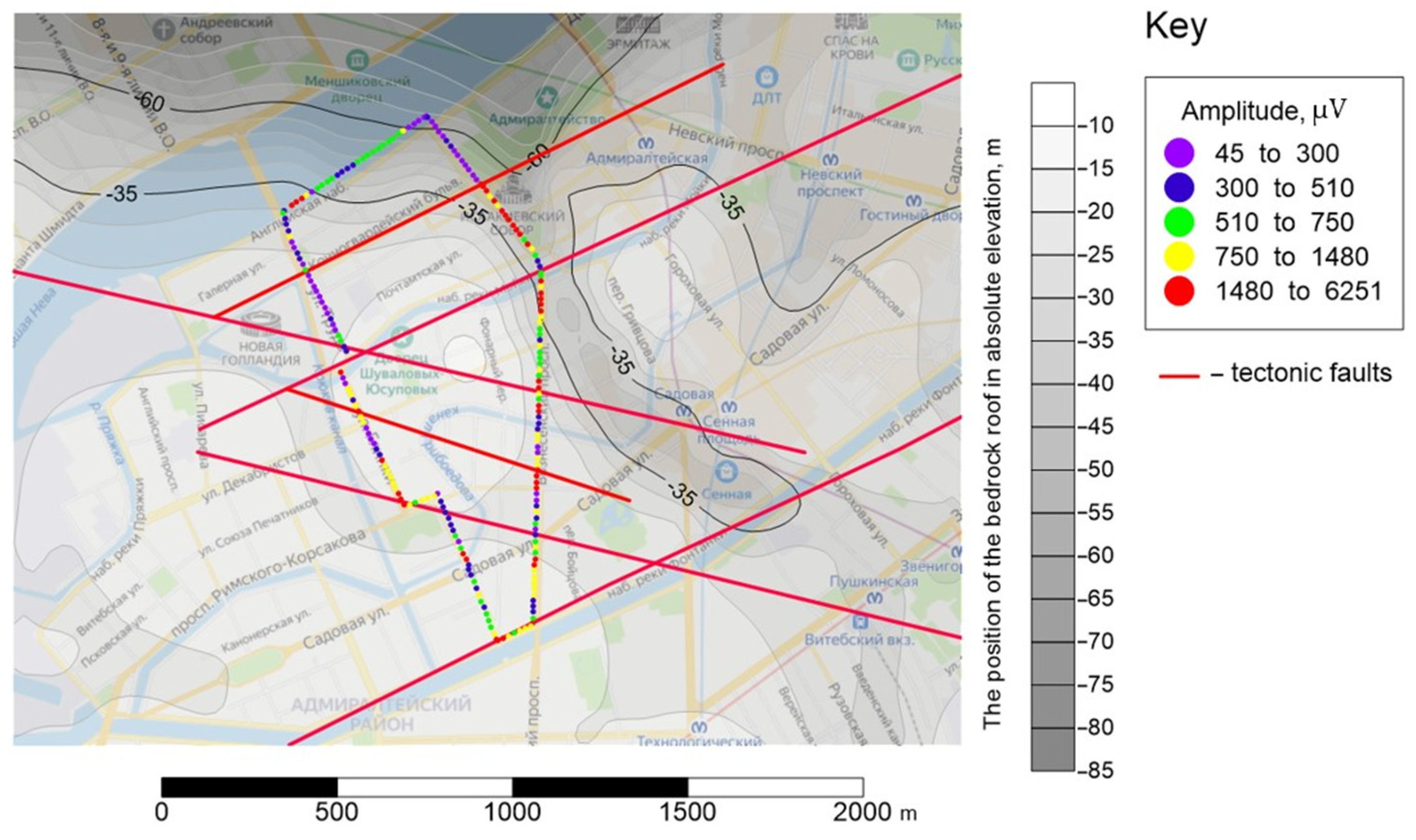
• City map;
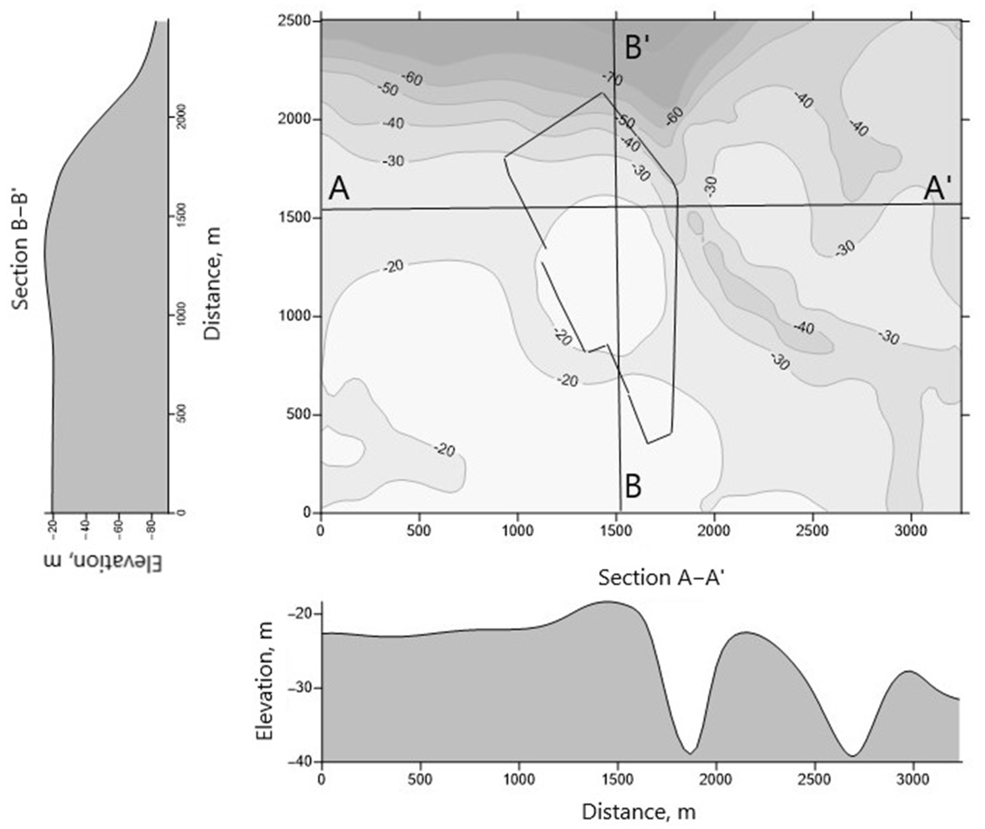
• Depth of bedrock;
• Tectonic map;
• Processed data of EMF measurements. reintegrated into the model.

The basis, demonstrating the depth of bedrock, was a map of the paleovalleys of St. Petersburg [18]. After digitizing and assigning the corresponding Z coordinates to the isolines, the data were presented in the form of a contour map (Figure 6).

Furthermore, the lines of tectonic faults and measurement points were integrated into the model (Figure 7).

The measurement points at this stage are visualized as five classes by means of a color scale, corresponding to intervals with an equal number of values. It is worth noting that this format does not allow one to fully assess the results of measurements to determine whether tectonics are active and whether there are anomalies of non-geological origin.

3. Results

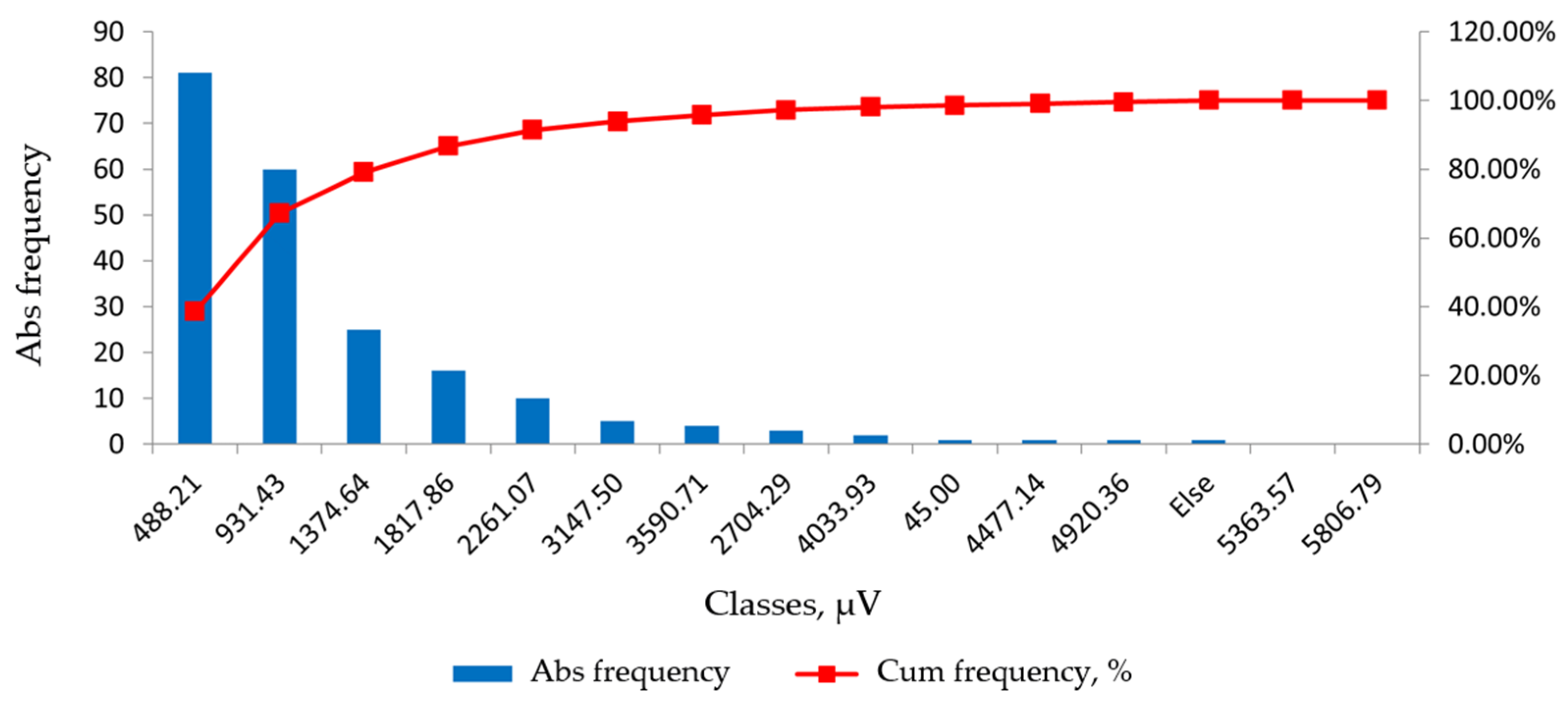
3.1. Statistical Description of Data and Construction of Variograms

A frequency analysis of the data distribution was applied to determine the regular and abnormal values of the voltages (μV). To construct histograms, the results obtained were divided into classes. A total of 14 classes were defined, as shown in

Table 3. Frequency distribution by class.

	Classes, µV	FA	FR	FC
1	488.21	81	0.0048	0.00
2	931.43	60	0.3857	0.39
3	1374.64	25	0.2857	0.68
4	1817.86	16	0.1190	0.80
5	2261.07	10	0.0762	0.87
6	3147.50	5	0.0476	0.92
7	3590.71	4	0.0143	0.93
8	2704.29	3	0.0238	0.96
9	4033.93	2	0.0190	0.98
10	45.00	1	0.0095	0.986
11	4477.14	1	0.0048	0.990
12	4920.36	1	0.0048	0.995
13	Else *	1	0.0000	0.995
14	5363.57	0	0.0000	0.995

*—the highest value.

.

After collecting the data, Exploratory Data Analysis was carried out. The analysis included the determination of absolute (F_A), relative (F_R), and cumulative (F_C) frequencies, followed by the construction of the corresponding histograms (Figure 8).

As can be seen from the histogram, the most frequent U values for this profile are the values of the first class—values in the range of 45 µV to 489 µV. U values of the second class—values in the range of 489 µV to 931.4 µV—occur with a 10% lower frequency than the values of the first class. According to an earlier analysis of 1400 U values for the city of St. Petersburg, it was determined that, with such a spread in values, the first two classes are considered as regular values due to the standard ENPEMF parameters of the studied area (see Section 2.1.), and the values from the third class can be referred to as anomalous U values due to local changes in the ENPEMF parameters. Thus, it was found that the anomalous profile values start from 931 µV.

Due to the fact that a significant deviation in the EMF value was revealed in different parts of the profile, it was decided to divide the profile into two parts—northeastern (NE) and northwestern (NW), the analysis results of which are presented in

Table 4. Frequency distribution by class.

№	Parameter	Profile	NE	NW
1	Mean, m, µV	928.50	1039.85	949.80
2	Median, M, µV	630.00	545.00	720.00
3	Std. dev., µV	942.72	1041.60	820.06
4	Min., µV	45.00	45.00	170.00
5	Per. 25, µV	322.50	247.50	420.00
6	Per. 50, µV	630.00	545.00	720.00
7	Per. 75, µV	1100.00	1062.50	1115.00
8	Max., µV	6250.00	6250.00	4800.00
9	1st absolute frequency value, µV	488 (1st class)	620 (1st class)	886 (2nd class)
10	Relative 1st frequency	38.5	55.4	31.6
11	2nd absolute frequency value, µV	931 (2nd class)	1240 (2nd class)	443 (1st class)
12	Relative 2nd frequency	28.5	22.3	28.5
13	3rd absolute frequency value, µV	1375 (3rd class)	1860 (3rd class)	1329 (3rd class)
14	Relative 3rd frequency	11.9	8.9	19.4

. Dividing was carried out on the basis of the main directions of tectonic faults in such a manner that each of the sub-bases contain information on measurements made through the tectonic faults of one direction (Figure 9). This profile allows doing this without additional complex manipulations.

The methodology for dividing the database into several sub-bases was not the ultimate goal of this study, since initially the goal was only to determine the efficiency of such an approach.

As it was found during the study, at frequency variations typical for the main profile and its northwestern part (NW), anomalous values start from the third frequency—from 931 µV and 886 µV and above, respectively. (The values for the NW part of the profile are inverted, since the first frequency does not correspond to the minimum voltage value). It is worth noting that the values belonging to the NW part of the profile are characterized by a high, most-common value, higher than in the entire profile and its NE part. The NE part of the profile is characterized by a different distribution of values—anomalous values start from the second frequency, at voltage values from 620 µV and above. Moreover, for the NE part of the profile, there is a significant increase in the voltage value on one of the linear parts. The operators also noticed this feature during the measurements. However, the attempts made to repeat the measurements gave similar results. Among the most likely sources of such a signal level, the government buildings located in this place, i.e., the Prosecutor’s Office and the Ministry of Justice, should be listed. Nonetheless, the nearby building of the Constitutional Court is not geographically connected with the area of high values. On the other hand, this place is characterized as difficult from a geological point of view, which is known in connection with St. Isaac’s Cathedral, which is experiencing a slow immersion and is a constant object of study for both geologists and surveyors [65,66].

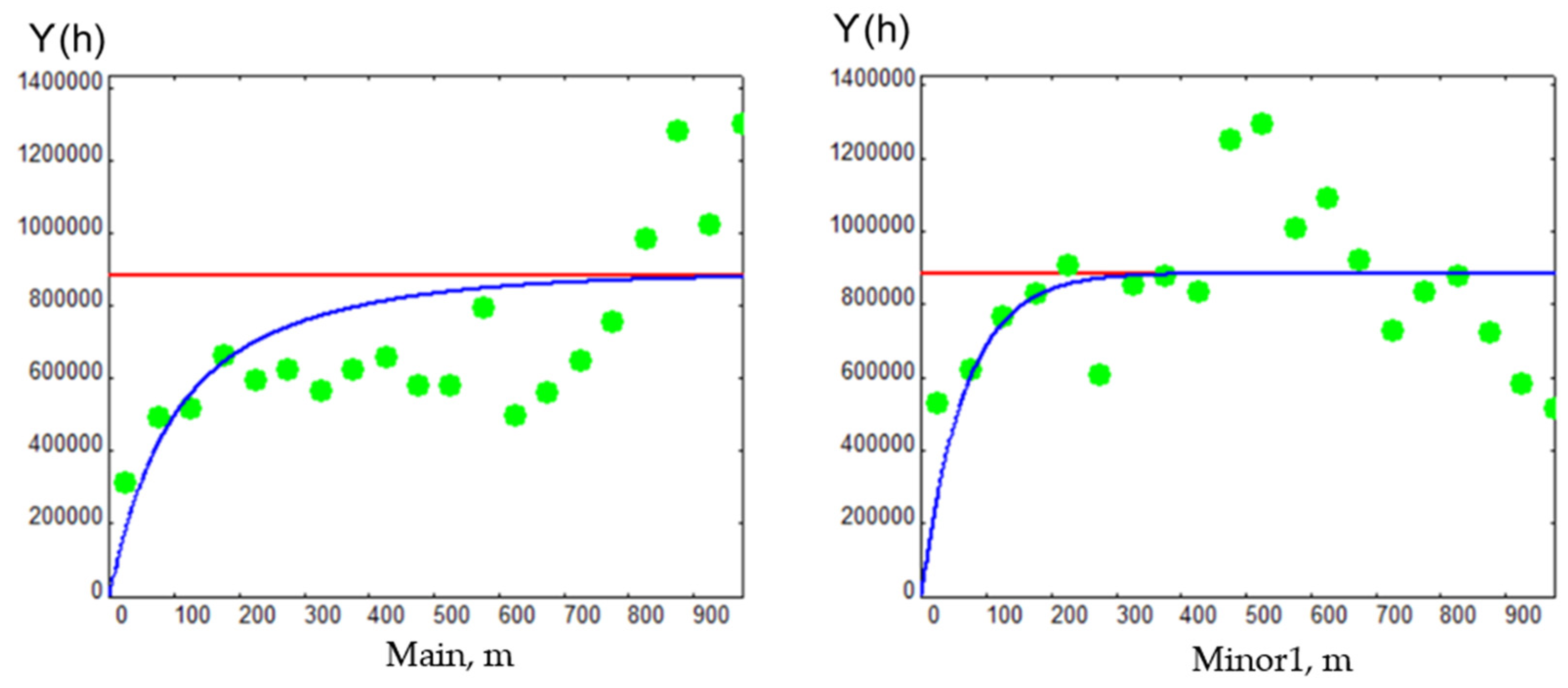
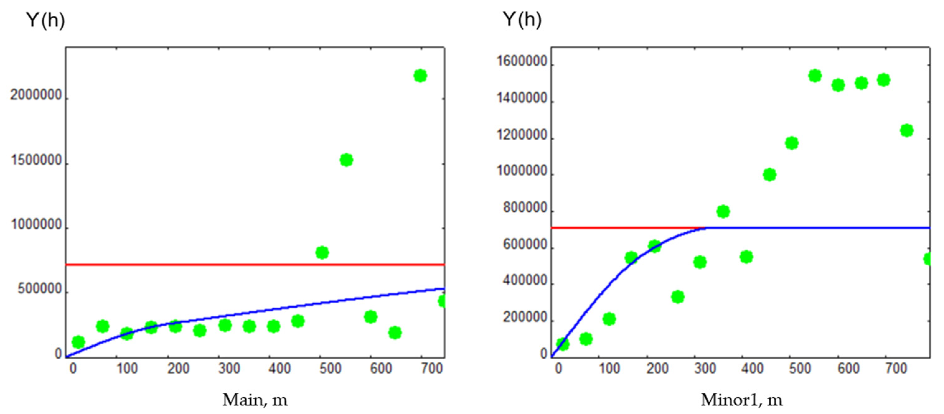
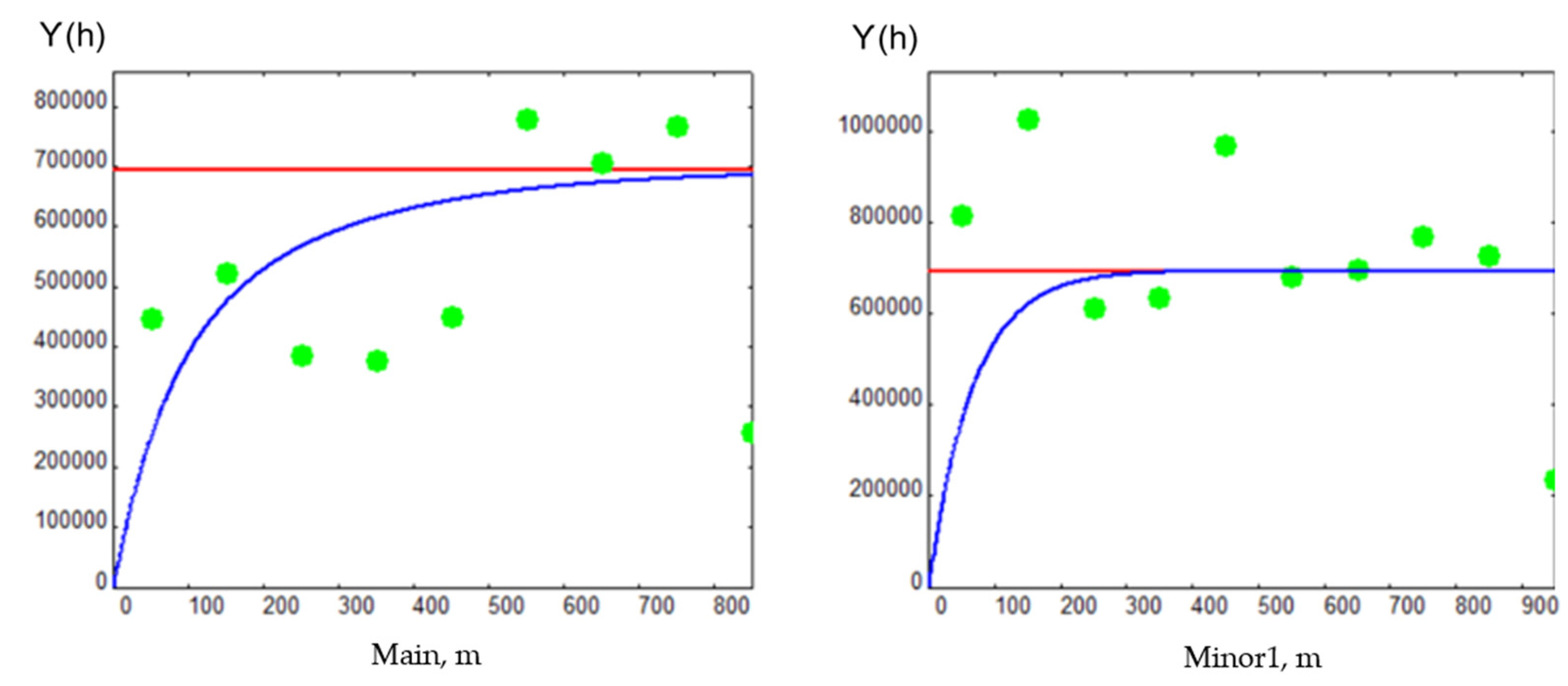
3.2. Geostatistical Analysis of Spatial Continuity: Variograms Estimation and Modeling

In this step, a geostatistical study of the data was carried out to characterize the spatial distribution of variable U for the entire study area. For the purpose of analysis and modeling spatial continuity, the variograms were calculated and modeled, for subsequent application in the kriging interpolation models [67]. The variograms summarize the main characteristics of the spatial continuity pattern of a physical phenomenon, the spatial dispersion of variable U, in particular:

• The large-scale spatial trend;
• The local spatial variogram anisotropy;
• The ranges of the spatial correlation of variable U.

It is necessary to determine the anisotropy ratio and main directions of spatial continuity as accurately as possible to ensure the quality of the spatial model. As is known, small ranges, which mean high variability at short distances, will result in the appearance of smooth interpolated images, and too large a range will result in artificial patterns, mainly in areas with a lack of data. The optimal choice for the anisotropy range’s value is based on the analysis of the variogram conditioned by expert knowledge of physical phenomena [68].

Based on the analysis, three variograms were constructed (Figure 10, Figure 11 and Figure 12): a variogram for a full data array covering the entire area, and variograms for two distinct areas, the north and south parts.

According to the variograms, the direction of anisotropy is displayed for the following directions:

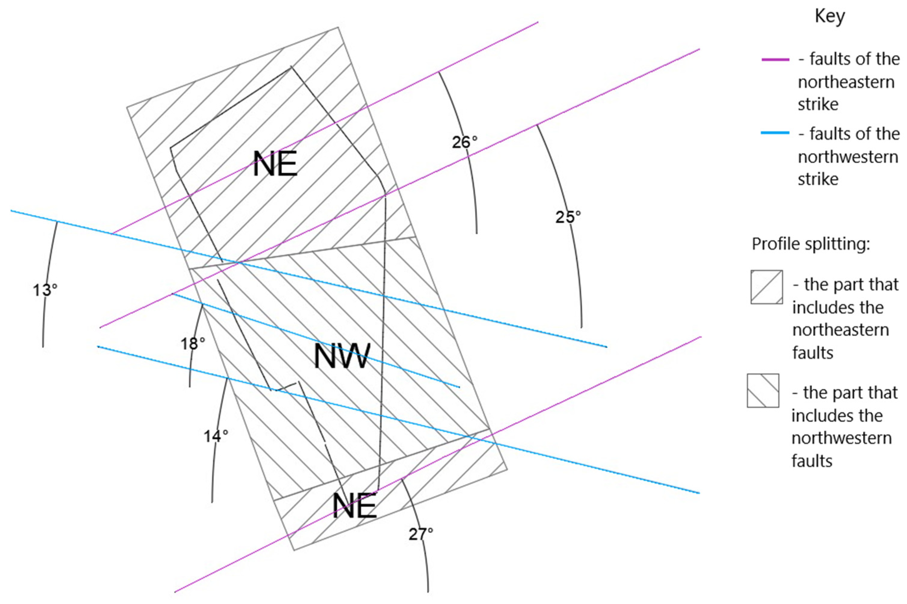
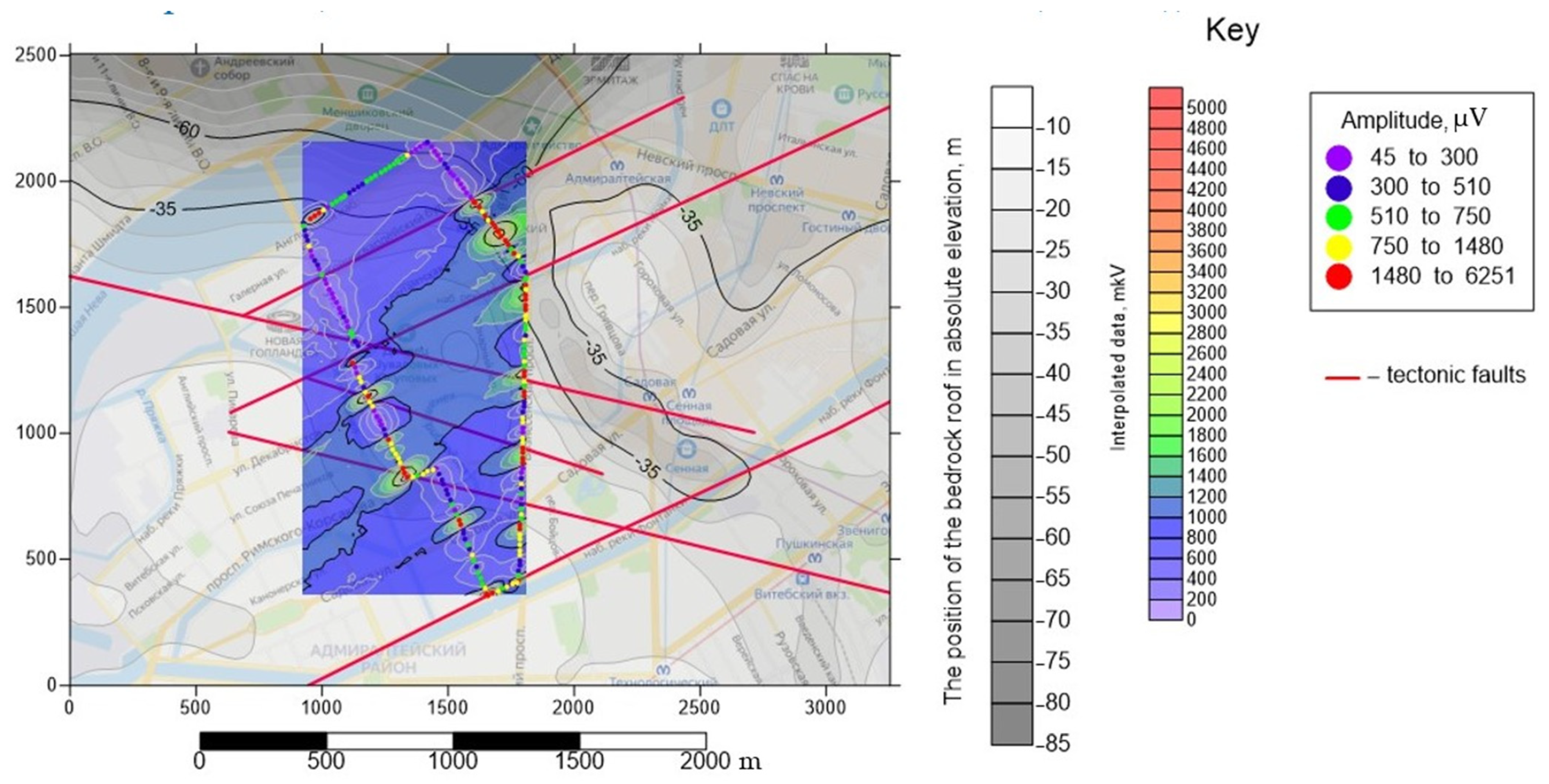
• For the entire area, the main direction of anisotropy corresponds to the azimuth of 31 degrees (counterclockwise rotation), Figure 10; this direction corresponds to three directions (27,25,26 degrees) of GDAFs. Other directions of GDAFs are not revealed by the variograms.
• After dividing the profiles into the two areas, the main directions of anisotropy are:

  2.1.

  NE—65 degrees; northeastern part, Figure 11;

  2.2.

  NW—31 degrees. northwestern part, Figure 12.

According to the results obtained, it can be concluded that the anisotropy directions are displayed partially or completely in the direction that is adjacent to the direction of GDAFs.

An exponential model was chosen to fit all the variograms, since spatial autocorrelation decreases exponentially with increasing distance. The variogram anisotropies were modeled by a common geometric anisotropy, defined, in 2D, by the ranges of the main direction and the perpendicular direction to the main one.

Table 5. Variography results.

N°	Parameter		Profile		NE		CW
			Real	Var *	Real *	Var *	Real *	Var *
1	Main direction, °			31	26	65	−15	31
2	Minor direction, °		-	121	-	155		121
Variogram
3	Ranges, m	Main	800		700		800
		Minor	380		300		400
4	Sill	Main	884,493		710,267		694,520
		Minor
5	Nugget effect	Main	-		-		-
		Minor

*—mean values.

presents the results of the analysis of the obtained variograms and the spatial direction of GDAFs (positive directions were taken into account counterclockwise according to the trigonometric circle).

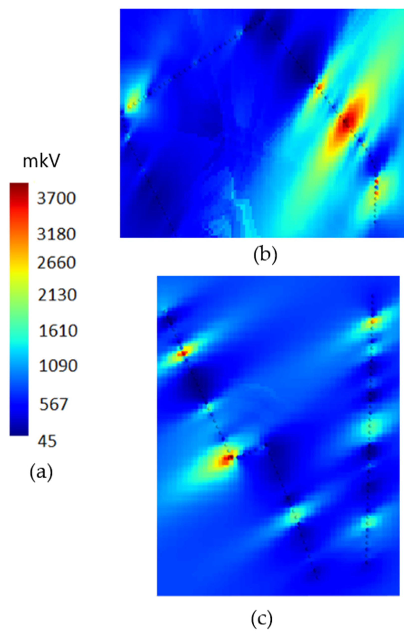
3.3. Kriging Maps

Based on the variogram models, the following kriging maps were built (Figure 13 and Figure 14) by using the variogram models of Section 3.2 and the U data. The Surfer [64] and GEOMS2 software packages were used for the estimation of kriging maps. GEOMS2 is a free software product (GNU General Public License version 3.0 (GPLv3)).

As one can see from the kriged maps (Figure 13), the main spatial patterns follow the main variogram spatial structures, which do not correspond to the directions of faults. According to the results obtained, the following conclusions can be drawn:

• The construction of a spatial model of profiles with an irregular grid with a pronounced geometric shape and high concentration of data along the profile perimeter is difficult to implement. There is only one spatial trend that coincides with only one global direction of GDAFs (northeast 26°). This can be explained by the difference in anomalous values. In addition, in the northeast direction, there is a dense accumulation of anomalous values in the area of St. Isaac’s Cathedral (see the description above).
• Dividing the profile into northeastern and northwestern sectors did not result in the initially expected results (Figure 14). The reason for the resulting trends is a non-standard, open, irregular grid of data with a big, empty, no-data space within the study area. It makes it very hard to assume the sample data values are spatially representative of the study area. It is necessary to conduct additional studies to collect more data in the “empty” sections of the profile measured by the EMP method, for which it is possible to build a more accurate spatial model without changing the approach to the method implementation.
• Significant spatial variation in anomalous values gives rise to problems during modeling. According to the conducted studies, the U values that correspond to GDAFs may belong to different classes, and a correlation between these classes (for example, between values of 600 µV and 900 µV) may be difficult to find without additional analysis, and potentially the subsequent selection of the correction coefficient allows us to make the transition from the actual measurement data to more convenient values associated with the classes. Moreover, anomalous values of class three and higher (depending on the profile, classes may vary) should have a 100% correlation in terms of displaying GDAFs, which also requires the introduction of additional correction coefficients for sample data.

4. Discussion

Despite the fact that dividing the database into sub-bases by the direction of the strike of tectonic faults has proved to be a promising method, the proposed approach still requires the addressing of some related problems. In particular, it is necessary to take into account those EMF values, the overestimated level of which is associated with the technogenic source. The solution to this problem can be the replacement of the amplitude data in µV with a special dimensionless correction coefficient. Furthermore, the introduction of such a correction coefficient will help to solve the problems of the interpolation clarity and displaying GDAFs in the model in conditions of a significant difference in measurements of the EMF value associated with tectonic faults having different coordinates. The features of filtering a man-made signal and anomalies of different levels must be considered separately. Within the framework of this study, such a scope of work cannot be presented. Thus, the development of such a correction coefficient may become the topic of further research.

In addition, for a widespread application of the method, it is necessary to adapt it to work with profiles in tectonically highly disturbed areas, as well as in areas where it is difficult to group tectonics into sub-bases.

When analyzing variograms for which constant coefficients corresponding to only two values, regular and anomalous, were introduced, the main direction of anisotropy did not correspond to the direction of GDAFs as well, but was co-directional with the direction of the spatial trend for all classes of values. If the value belonged to the range of 0 to the anomalous value, then a coefficient of 0 was assigned; if the value was equal to the anomalous value and exceeded it, then the coefficient value was equal to 1. Regular and anomalous values were determined based on frequency diagrams and correspond to 931 µV, 620 µV and 886 µV for the main profile and sub-bases.

The discrepancy between the main correlation direction when dividing the database into sub-bases can be explained by the following reasons:

• the lack of data on one of the linear parts of the profile. The solution to this problem can only be the introduction of additional profiles;
• the lack of correlation between values belonging to different classes. The solution to this problem, as mentioned earlier, can be the introduction of additional correction coefficients reflecting the belonging of the value to normal or anomalous levels or classes.

Moreover, in the future, it is necessary to take into account man-made sources (subway, substations, etc.) in the model, as well as welding sites outside GDAF zones, because repeated pipe breaks often occur in such places.

Thus, the main directions of further research are the following: the development of a correction coefficient that allows the separating of anomalous values of all levels from regular ones; work on filling the model; development of a measurement technique taking into account newly identified data features; further statistical processing of data.

5. Conclusions

In this research, an attempt was made to find an approach to the spatial modelling of data characterized by location along a perimeter with a complex geometric shape and two directions of data anisotropy, as well as by step transition from high values to low.

In the course of the study, the tentative attempt to create a spatial model of the ENPEMF measurement data did not allow for determining an unambiguous methodological approach to such data visualization, but made it possible to reveal the main challenges of the existing databases. The solution to which will allow us to approach the solution to the main issue.

First of all, the main problem of the processed data is the absence of measurement points inside the profile with their high density around the perimeter. It was established that it is necessary to introduce amendments to the technique of detecting the location of GDAFs by the EMP method. There are two potentially possible options: changing the monitoring network for this method; introducing limitations for the method’s applicability, which are based on defining the maximum permissible distance between measurement points. The second option requires additional research to find the maximum permissible distances. It is worth noting that these amendments should be developed specifically for the urban environment and large areas with a complex building system. At the same time, options must meet both the requirements for identifying GDAFs (equally with the adopted profiling technique using a dense line of measurements across tectonic faults), and the requirements for auxiliary points when constructing a kriging network. Both possible options require additional research.

Secondly, the splitting of the profile into sub-bases did not provide the expected result. The expected azimuths of anisotropy did not coincide with the calculated ones. The most probable explanation is the high heterogeneity of the data. Therefore, establishing the method of dividing the profile into sectors also requires additional research aimed at finding the optimal division criteria and limitations of the applicability of the dividing method. Furthermore, to solve this problem, it is necessary to conduct research on determining the coefficients, which will allow the interpolation of data between anomalous values of different levels (classes).

Further development of the proposed methods will facilitate the further modelling of profiles such as those obtained in the linear profiling mode, characterized by step differences and described by multiple directions of anisotropy. Similar data are typical for Earth sciences.

The results of this research will contribute to improving the efficiency of the designing of underground utilities and reduce the accident rate involving underground utilities by means of the early repair of pipeline sections located in zones of geodynamically active faults. The obtained spatial models can be used as the basis for planning the repairs in underground utilities, which in turn will reduce the probability of accidents, the consequences of which may not only result in changes in traffic patterns, transport collapses, and road accidents, but also human and economic losses. The circumstances listed above correspond to one of the 17 Sustainable Development Goals, namely Goal 9, “Build resilient infrastructure, promote sustainable industrialization and foster innovation”, Target 9.1: “Develop quality, reliable, sustainable and resilient infra-structure, including regional and transborder infrastructure, to support economic development and human well-being, with a focus on affordable and equitable access for all”. It should also be noted that, in addition to the positive impact on infrastructure, monitoring of pipelines will reduce the negative impact on the environment, which is especially relevant for St. Petersburg due to the proximity of the Gulf of Finland. It also corresponds to Goal 11 “Sustainable cities and communication”, Target 11.6 “By 2030, reduce the adverse per capita environmental impact of cities, including by paying special attention to air quality and municipal and other waste management”.

References

- Alekseenko, V.A.; Pashkevich, M.A.; Alekseenko, A.V. Metallisation and environmental management of mining site soils. J. Geochem. Explor. 2017, 174, 121–127. [Google Scholar] [CrossRef]
- Yurak, V.V.; Dushin, A.V.; Mochalova, L.A. Vs sustainable development: Scenarios for the future. J. Min. Inst. 2020, 242, 242. [Google Scholar] [CrossRef]
- Shklyarskiy, Y.; Hanzelka, Z.; Skamyin, A. Experimental study of harmonic influence on electrical energy metering. Energies 2020, 13, 5536. [Google Scholar] [CrossRef]
- Bykowa, E.; Dyachkova, I. Modeling the size of protection zones of cultural heritage sites based on factors of the historical and cultural assessment of lands. Land 2021, 10, 1201. [Google Scholar] [CrossRef]
- Litvinenko, V.S.; Tsvetkov, P.S.; Dvoynikov, M.V.; Buslaev, G.V. Barriers to implementation of hydrogen initiatives in the context of global energy sustainable development. J. Min. Inst. 2020, 244, 428–438. [Google Scholar] [CrossRef]
- Goldobina, L.A.; Demenkov, P.A.; Trushko, O.V. Ensuring the safety of construction works during the erection of buildings and structures. J. Min. Inst. 2019, 239, 583–595. [Google Scholar] [CrossRef] [Green Version]
- Redko, I.; Ujma, A.; Redko, A.; Pavlovskiy, S.; Redko, O.; Burda, Y. Energy efficiency of buildings in the cities of Ukraine under the conditions of sustainable development of centralized heat supply systems. Energy Build. 2021, 247, 110947. [Google Scholar] [CrossRef]
- Tchórzewska-Cieślak, B.; Pietrucha-Urbanik, K.; Eid, M. Functional safety concept to support hazard assessment and risk management in water-supply systems. Energies 2021, 14, 947. [Google Scholar] [CrossRef]
- Golovina, E.; Pasternak, S.; Tsiglianu, P.; Tselischev, N. Sustainable management of transboundary groundwater resources: Past and future. Sustainability 2021, 13, 12102. [Google Scholar] [CrossRef]
- Möderl, M.; Kleidorfer, M.; Sitzenfrei, R.; Rauch, W. Identifying weak points of urban drainage systems by means of VulNetUD. Water Sci. Technol. 2009, 60, 2507–2513. [Google Scholar] [CrossRef]
- Iakovleva, E.; Belova, M.; Soares, A. Allocation of potentially environmentally hazardous sections on pipelines. Geosciences 2021, 11, 3. [Google Scholar] [CrossRef]
- Dashko, R.E.; Alekseev, I.V. Main features of engineering-geological and geotechnical research of microbiota influence on hard rocks in the urban underground space. In Proceedings of the International Multidisciplinary Scientific GeoConference Surveying Geology and Mining Ecology Management, SGEM, Sofia, Bulgaria, 30 June–6 July 2019; Volume 19, pp. 369–376. [Google Scholar] [CrossRef]
- Singh, J.; Singh, S.; Pal Singh, J. Investigation on wall thickness reduction of hydropower pipeline underwent to erosion-corrosion process. Eng. Fail. Anal. 2021, 127, 105504. [Google Scholar] [CrossRef]
- Kiselev, V.; Guseva, N.; Kuranov, A. Creating Forecast Maps of the Spatial Distribution of Dangerous Geodynamic Phenomena Based on the Principal Component Method. IOP Conf. Ser. Earth Environ. Sci. 2021, 666, 032071. [Google Scholar] [CrossRef]
- Malyshkov, S.Y.; Gordeev, V.F.; Pustovalov, N.A. Detailing the tectonic structure of a nuclear industry construction site using an earth’s natural pulsed electromagnetic field method. IOP Conf. Ser. Earth Environ. Sci. 2018, 211, 012077. [Google Scholar] [CrossRef] [Green Version]
- Tan, Z.; Yang, Y.; Chen, W.; Li, S. Large deformation control technology of high geostress soft rock tunnel of China-Laos railway. J. China Railw. Soc. 2020, 42, 171–178. [Google Scholar] [CrossRef]
- Koteleva, N.; Frenkel, I. Digital Processing of Seismic Data from Open-Pit Mining Blasts. Appl. Sci. 2021, 11, 383. [Google Scholar] [CrossRef]
- Tao, M.; Hong, Z.; Peng, K.; Sun, P.; Cao, M.; Du, K. Evaluation of excavation-damaged zone around underground tunnels by theoretical calculation and field test methods. Energies 2019, 12, 1682. [Google Scholar] [CrossRef] [Green Version]
- Shabarov, A.N.; Goncharov, E.V.; Lazarevich, T.I.; Zolotykh, S.S. Prediction of high methane-recovery regions and gas extraction technology based on geodynamic zoning of bowels. J. Min. Sci. 2003, 39, 41–46. [Google Scholar] [CrossRef]
- Kiselev, V.A.; Guseva, N.V. Geodynamic zoning of the Kuzbass territory based on the integrated analysis of the cartographic material. Asia Life Sci. 2019, 1, 275–286. [Google Scholar]
- Alekseev, A.V.; Iovlev, G.A. Adjustment of hardening soil model to engineering geological conditions of Saint-Petersburg. Min. Inf. Anal. Bull. 2019, 2019, 75–87. [Google Scholar] [CrossRef]
- Kostenko, B.V.; Larionov, R.I. Field data analysis in construction of escalator tunnels at Obvodny Kanal and Admiralteyskaya stations of the Saint-Petersburg Metro using tunnel boring machine. Min. Inf. Anal. Bull. 2021, 2021, 48–64. [Google Scholar] [CrossRef]
- Zmiievska, K.; Tubaltsev, O.; Zmiievskyi, A. Application of the method of observing the natural impulse electromagnetic field of the earth to trace watered faults on the example of yeristovo quarry. In Proceedings of the E3S Web of Conferences, Dnipro, Ukraine, 9 July 2019; Volume 109. [Google Scholar] [CrossRef]
- De Andrade, H.D.; De Figuêiredo, A.L.; Fialho, B.R.; Da Paiva, J.L.S.; De Queiroz Júnior, I.S.; Sousa, M.E.T. Analysis and development of an electromagnetic exposure map based in spatial interpolation. Electron. Lett. 2020, 56, 373–375. [Google Scholar] [CrossRef]
- Nekhoroshih, D.S.; Demyanov, V.V.; Kanevsky, M.F.; Chernov, S.Y.; Savelyeva, E.A. Stochastic models-reduction of spatially distributed data on the environment. Preprint No. IBRAE 2000, 5, 1–28. (In Russian) [Google Scholar]
- Castelo Branco, R.M.G.; de Castro, N.A.; Leopoldino Oliveira, K.M.; Monteiro Santos, F.A.; Almeida, E.P.; da Silva, F.M.; Castelo Branco, J.L. Mapping the basement architecture using magnetotelluric data across a coastal part of the Borborema structural province, Ceará—Brazil. J. S. Am. Earth Sci. 2021, 112, 103525. [Google Scholar] [CrossRef]
- Danilov, A.; Pivovarova, I.; Krotova, S. Geostatistical analysis methods for estimation of environmental data homogeneity. Sci. World J. 2018, 2018, 7424818. [Google Scholar] [CrossRef] [Green Version]
- Li, D.; Yu, N.; Li, X.; Wang, E.; Li, R.; Wang, X. Magnetotelluric evidence of fluid-related seismicity beneath the Chuxiong Basin, SE Tibetan Plateau. Tectonophysics 2021, 816, 229039. [Google Scholar] [CrossRef]
- Al Shawa, O.; Atzori, S.; Doglioni, C.; Liberatore, D.; Sorrentino, L.; Tertulliani, A. Coseismic vertical ground deformations vs. intensity measures: Examples from the Apennines. Eng. Geol. 2021, 293, 106323. [Google Scholar] [CrossRef]
- GhojehBeyglou, M. Geostatistical modeling of porosity and evaluating the local and global distribution. J. Pet. Explor. Prod. Technol. 2021, 11, 4227–4241. [Google Scholar] [CrossRef]
- Available online: https://www.google.ru/maps/@59.9598569,30.3217566,11.34z?hl=ru (accessed on 10 December 2021).
- Available online: http://www.vidiani.com/political-map-of-russia/ (accessed on 10 December 2021).
- Terekhov, E.N.; Kolodyazhny, S.Y.; Baluev, A.S.; Okina, O.I. Local geochemical features of lower paleozoic rocks in the area of duderhof dislocations (north-west of the russian plate). Lithosphere 2021, 21, 5–22. [Google Scholar] [CrossRef]
- Dashko, R.E.; Aleksandrova, O.Y.; Kotiukov, P.V.; Shidlovskaya, A.V. Special aspects of geotechnical conditions of St. Petersburg. Urban Dev. Geotech. Constr. 2011, 1, 1–47. (In Russian) [Google Scholar]
- Lebedeva, Y.; Kotiukov, P.; Lange, I. Study of the geo-ecological state of groundwater of metropolitan areas under the conditions of intensive contamination thereof. J. Ecol. Eng. 2020, 21, 157–165. [Google Scholar] [CrossRef]
- Mulev, S.N.; Starnikov, V.N.; Romanevich, O.A. The current stage of development of the geophysical method for recording natural electromag neticra diation (EEMI—NER). Ugol 2019, 10, 6–14. [Google Scholar] [CrossRef]
- Rabinovitch, A.; Frid, V.; Bahat, D. Use of electromagnetic radiation for potential forecast of earthquakes. Geol. Mag. 2018, 155, 992–996. [Google Scholar] [CrossRef]
- Simpson, F.; Bahr, K. Practical magnetotellurics. Pract. Magnetotell. 2005, 1–254. [Google Scholar] [CrossRef]
- Sabaka, T.J.; Olsen, N.; Purucker, M.E. Extending comprehensive models of the earth’s magnetic field with ørsted and CHAMP data. Geophys. J. Int. 2004, 159, 521–547. [Google Scholar] [CrossRef]
- Lukovenkova, O.; Senkevich, Y.; Solodchuk, A.; Shcherbina, A. Overview of processing and analysis methods for pulse geophysical signals. In Proceedings of the XI International Conference Solar-Terrestrial Relations and Physics of Earthquake Precursors, Kamchatka, Russia, 22–25 September 2020; Volume 196. [Google Scholar] [CrossRef]
- Bespal’ko, A.A.; Yavorovich, L.V.; Eremenko, A.A.; Shtirts, V.A. Electromagnetic Emission of Rocks after Large-Scale Blasts. J. Min. Sci. 2018, 54, 187–193. [Google Scholar] [CrossRef]
- Resolution of the Government of St. Petersburg Dated 11 December 2013 N 989 on the Approval of the Water Supply and Sewerage Scheme for St. Petersburg for the Period until 2025, Taking into Account the Prospects until 2030; Government of St. Petersburg: St. Petersburg, Russia, 2013.
- Melnikov, E.K.; Shabarov, A.N. Assessment of the role of the geodynamic factor in the accident rate of pipeline systems. J. Min. Inst. 2010, 188, 203–206. (In Russian) [Google Scholar]
- Melnikov, E.K.; Mustafin, M.G.; Snareva, M.M. Methods for organizing geodetic control of water pipe deformations in St. Petersburg. Mine Surv. Bull. 2013, 3, 43–47. (In Russian) [Google Scholar]
- Hao, G.; Wang, H. Study on Signals Sources of Earth’s Natural Pulse Electromagnetic Fields. In Computational Intelligence and Intelligent Systems. ISICA 2012. Communications in Computer and Information Science; Li, Z., Li, X., Liu, Y., Cai, Z., Eds.; Springer: Berlin/Heidelberg, Germany, 2012; Volume 316. [Google Scholar] [CrossRef]
- Panfilov, A.A. Electrical phenomena under dynamic impact on rock samples. Sci. J. KubGAU 2012, 81, 1–14. (In Russian) [Google Scholar]
- Kataev, S.G.; Dolgy, M.E. About a natural pulse electromagnetic field of earth. In Proceedings of the 12th Conference and Exhibition Engineering Geophysics, Anapa, Russia, 25–29 April 2016; pp. 165–175. [Google Scholar]
- Vorobyov, A.A.; Zavadovskaya, E.K.; Salnikov, V.N. Report of the Academy of Science of the USSR; USSR: Moscow, Russia, 1975; Volume 220, pp. 82–85. (In Russian) [Google Scholar]
- Haji, T.A.; Moumni, Y.; Msaddek, M.H. Fault-style analysis and seismic interpretation: Implications for the structural issues of the South-eastern Atlas in Tunisia. J. Afr. Earth Sci. 2020, 172, 103962. [Google Scholar] [CrossRef]
- Rudianov, G.V.; Krapivskii, E.I.; Danil’ev, S.M. Evaluation of signal properties when searching for cavities in soil under concrete slabs by radio detection stations of subsurface investigation. J. Min. Inst. 2018, 231, 245. [Google Scholar] [CrossRef]
- Popov, A.L.; Parkhimchik, M.V.; Senchina, N.P.; Idiyatullin, M.M. Localization of potentially dangerous zones of rock mass based on the results of studying natural electromagnetic radiation. Innovative directions in the design of mining enterprises: Geomechanical support for the design and support of mining operations. In Proceedings of the VIII International Scientific and Practical Conference; Collection of scientific papers; Saint Petersburg Mining University: Saint Petersburg, Russia, 2017; pp. 213–219. (In Russian) [Google Scholar]
- Abreha, D.A. Analysing Public Transport Performance Using Efficiency Measures and Spatial Analysis; The Case Study of Addis Ababa, Ethiopia. Master’s Thesis, International Institute for Geo-Information Science and Earth Observation, Enschede, The Netherlands, 2007. [Google Scholar]
- Bolt, A.B.; Scott, R.W.; Horn, W.L.; MacDonald, G.A. Geological Elements: Earthquakes, Tsunamis, Volcanic Eruptions, Avalanches, Landslides, Floods; Mir: Moscow, Russia, 1978; p. 444. [Google Scholar]
- Dolgiy, M.E.; Kataev, S.G. Study of the natural pulsed electromagnetic field of the Earth. Vestn. Tomsk. Gos. Univ. Mat. Mekh. 2015, 2, 61–70. (In Russian) [Google Scholar]
- Agranat, I.V. Prospects of research of natural electromagnetic radiation of very low frequency. Research in the field of earth sciences. In Proceedings of the IX Regional Youth Scientific Conference “Research in the Field of Earth Sciences”, Petropavlovsk-Kamchatsky, Russia, 1–2 December 2011; pp. 139–152. (In Russian). [Google Scholar]
- Schmucker, U. An introduction to induction anomalies. J. Geomagn. Geoelect. 1970, 22, 9–33. [Google Scholar] [CrossRef] [Green Version]
- Frid, V.; Wang, E.Y.; Mulev, S.N.; Li, D.X. The fracture induced electromagnetic radiation: Approach and protocol for the stress state assessment for mining. Geotech. Geol. Eng. 2021, 39, 3285–3291. [Google Scholar] [CrossRef]
- Sadovskii, V.M.; Sadovskaya, O.V.; Efimov, E.A. Analysis of seismic waves excited in near-surface soils by means of the electromagnetic pulse source “Yenisei”. Mater. Phys. Mech. 2019, 42, 544–557. [Google Scholar] [CrossRef]
- Tsirel’, S.V. Attenuation and change in the shape of stress waves in rocks. J. Min. Sci. 1993, 28, 338–341. [Google Scholar] [CrossRef]
- Popov, S.V.; Kashkevich, M.P.; Kashkevich, V.I.; Kharitonov, V.V.; Yovenko, E.V. Absorption of UHF electromagnetic waves in the water of Lake Ladoga (Leningrad region). Arct. Antarct. Probl. 2017, 2, 43–49. [Google Scholar] [CrossRef]
- Pietroń, J.; Chalov, S.R.; Chalova, A.S.; Alekseenko, A.V.; Jarsjö, J. Extreme spatial variability in riverine sediment load inputs due to soil loss in surface mining areas of the Lake Baikal basin. Catena 2017, 152, 82–93. [Google Scholar] [CrossRef]
- Dzhioeva, A.K.; Brigida, V.S. Spatial non-linearity of methane release dynamics in underground boreholes for sustainable mining. J. Min. Inst. 2020, 245, 522–530. [Google Scholar] [CrossRef]
- Witte, R.S.; Witte, J.S. Statistics, 11th ed.; Wiley: Hoboken, NJ, USA, 2016; p. 496. [Google Scholar]
- Available online: https://www.goldensoftware.com/blog/surfer-13-new-feature-series-graticules (accessed on 10 December 2021).
- Dashko, R.E.; Salnikov, P.M. Main principles of an integral monitoring for St. Isaac’s cathedral in Saint Petersburg. Topical Issues of Rational Use of Natural Resources. In Proceedings of the International Forum-Contest of Young Researchers, St. Petersburg, Russia, 18–20 April 2018; pp. 17–22. [Google Scholar]
- Dashko, R.E.; Shidlovskaya, A.V.; Aleksandrova, O.Y.; Alekseev, I.V. Engineering-geological and hydrogeological problems of substantiating the long-term stability of St. Isaac’s Cathedral (St. Petersburg). J. Min. Inst. 2012, 195, 28. [Google Scholar]
- Goovaerts, P. Geostatistics for Natural Resource Evaluation; Oxford University Press: Oxford, UK, 1987. [Google Scholar]
- Saveliev, A.A.; Mukharamova, S.S.; Pilyugin, A.G.; Chizhikov, N.A. Geostatistical Analysis of Data in Ecology and Nature Management (Using the R Package); Kazan University: Kazan, Russia, 2012; p. 120. [Google Scholar]