Article

Temporal and Spatial Analysis of PM2.5 and O3 Pollution Characteristics and Transmission in Central Liaoning Urban Agglomeration from 2015 to 2020

College of New Energy and Environment, Jilin University, Changchun 130012, China
*
Author to whom correspondence should be addressed.
Sustainability 2022, 14(1), 511; https://doi.org/10.3390/su14010511
Submission received: 22 October 2021 / Revised: 27 December 2021 / Accepted: 27 December 2021 / Published: 4 January 2022
(This article belongs to the Collection Air Pollution Control and Sustainable Development)

Abstract

:
The central Liaoning urban agglomeration is an important heavy industry development base in China, and also an important part of the economy in northeast China. The atmospheric environmental problems caused by the development of heavy industry are particularly prominent. Trajectory clustering, potential source contribution (PSCF), and concentration weighted trajectory (CWT) analysis are used to discuss the temporal and spatial pollution characteristics of PM2.5 and ozone concentrations and reveal the regional atmospheric transmission pattern in central Liaoning urban agglomeration from 2015 to 2020. The results show that: (1) PM2.5 in the central Liaoning urban agglomeration showed a decreasing trend from 2015 to 2020. The concentration of PM2.5 is the lowest in 2018. Except for Benxi (34.7 µg/m3), the concentrations of PM2.5 in other cities do not meet the standard in 2020. The ozone concentration in Anshan, Liaoyang, and Shenyang reached the peaks in 2017, which are 68.76 µg/m3, 66.27 µg/m3, and 63.46 µg/m3 respectively. PM2.5 pollution is the highest in winter and the lowest in summer. The daily variation distribution of PM2.5 concentration showed a bimodal pattern. Ozone pollution is the most serious in summer, with the concentration of ozone reaching 131.14 µg/m3 in Shenyang. Fushun is affected by Shenyang intercity pollution, and the ozone concentration is high. (2) In terms of spatial distribution, the high values of PM2.5 are concentrated in monitoring stations in urban areas. On the contrary, the concentration of ozone in suburban stations is higher. The high concentration of ozone in the northeast of Anshan, Liaoyang, Shenyang to Tieling, and Fushun extended in a band distribution. (3) Through cluster analysis, it is found that PM2.5 and ozone in Shenyang are mainly affected by short-distance transport airflow. In winter, the weighted PSCF high-value area of PM2.5 presents as a potential contribution source zone of the northeast trend with wide coverage, in which the contribution value of the weighted CWT in the middle of Heilongjiang is the highest. The main potential source areas of ozone mass concentration in spring and summer are coastal cities and the Bohai Sea and the Yellow Sea. We conclude that the regional transmission of pollutants is an important factor of pollution, so we should pay attention to the supply of industrial sources and marine sources of marine pollution in the surrounding areas of cities, and strengthen the joint prevention and control of air pollution among regions. The research results of this article provide a useful reference for the central Liaoning urban agglomeration to improve air quality.

1. Introduction

With the rapid development of the social economy, air pollution has become an increasingly serious environmental problem. Epidemiological studies have found that long-term exposure to air pollution will increase the risk of disease. For example, fine particulate matter (PM2.5) is significantly associated with an increase in the prevalence of diabetes; short-term exposure to high concentrations of PM2.5 and ozone(O3) will increase cardiovascular disease, respiratory disease, and non-risk of accidental death [1,2,3]. Since 2013, regional atmospheric environmental problems mainly characterized by PM2.5 pollution have attracted widespread attention in China. Therefore, China has formulated and issued a series of policies to alleviate air pollution. From 2015 to 2020, PM2.5 pollution in China has been significantly reduced, while ozone pollution has become increasingly serious [4,5,6,7,8,9].
Central Liaoning Urban Agglomeration (CLUA) is located in the Northeast Plain. Due to the concentrated urban distribution, dense population, and industrial structure dominated by heavy industry, air pollution is serious. In 2020, the proportion of PM2.5 and O3 as the primary pollutants in Liaoning Province in the days exceeding the standard was 62.9% and 33.8% respectively. The annual average concentration of PM2.5 was 38 μg/m3 which exceeds the secondary standard of ambient air quality [10]. The air quality of Central Liaoning Urban Agglomeration may be affected by regional anthropogenic emissions. In winter, the transboundary pollution of PM2.5 is extremely significant. Some studies also found that there was regional transmission of pollutants in Central Liaoning Urban Agglomeration and Harbin-Changchun urban agglomeration [11,12]. Straw burning and coal-burning heating during winter resulted in heavy PM2.5 pollution, and the interannual change of PM2.5 in Northeast China showed an obvious upward trend from 1998 to 2016. MDA8 (maximum daily 8 h average) O3 increased and the number of days exceeding the standard continued to increase which can be attributed to the superimposed effects of atmospheric long-distance transport and anthropogenic emissions [13,14,15,16,17].
Many studies have mentioned the occurrence of air pollution in various urban agglomerations, such as the Beijing-Tianjin-Hebei region, Harbin-Changchun region, Yangtze River Delta, etc., while there are few studies on Northeast China and Central Liaoning Urban Agglomerations [18,19,20]. This study collected PM2.5 and O3 concentration data in CLUA (Anshan, Benxi, Fushun, Liaoyang, Shenyang, and Tieling) from 2015 to 2020 and analyzed its temporal and spatial characteristics to determine the level of pollutants. Specifically, the aim was to (1) study the long-term temporal and spatial changes of the mass concentrations of PM2.5 and O3 and (2), through the back trajectory HYSPLIT model and cluster analysis, discuss the regional transportation of PM2.5 and ozone in Shenyang, which is the center of Central Liaoning Urban Agglomeration, in order to provide a useful reference for CLUA to improve air quality.

2. Data Sources and Methods

2.1. Data Sources

The geographical location of the study area is shown in Figure 1. This study used in situ data from a total of 38 air quality monitoring stations (Table 1) in six cities in central Liaoning urban agglomeration from 2015 to 2020 (http://www.cnemc.cn/ accessed on 14 May 2021). Among them, O3 data used ozone eight-hour moving average (O3-8 h), and PM2.5 used hourly monitoring data. Ozone is measured by UV spectrophotometry (Thermo Scientific Model 49iQ Ozone Analyzer). PM2.5 is passed β X-ray absorption method and light scattering method were used for real-time determination (Thermo Scientific Model 5030i Sharp Particulate Monitor). The season division refers to the meteorological industry-standard “Climate Season Division” (QX/T152-2012) and the annual difference is adjusted. The results are: spring (1 April–31 May), summer (1 June–31 August), autumn (1 September–31 October), winter (1 November–31 March of the following year).

2.2. Research Method

The Geographical Information System (GIS)-TrajStat software is used for backward trajectory clustering, potential source contribution analysis, and concentration weighted trajectory analysis, and grids were divided by 1° × 1° within the trajectory range [21,22].

2.2.1. Cluster Analysis

The Hybrid Single Particle Lagrangian Integrated Trajectory (HYSPLIT) model (http://ready.arl.noaa.gov/HYSPLIT.php accessed on 12 July 2021) developed by the National Oceanic and Atmospheric Administration (NOAA) was used to simulate 72 h backward trajectories at 100 m altitude for Shenyang to analyze atmospheric pollutant transportation [23,24].
In the study, to understand the regional transport processes effects, we used 1° × 1° Global Data Assimilation System (GDAS) data from National Centers for Environmental Prediction (NCEP). We also calculated the 72 h backward airflow trajectory at 0:00, 6:00, 12:00, and 18:00 every day from 2015 to 2020. Euclidean classification method is used to analyze the transport path of regional air mass through data statistics of various trajectories after clustering, which can distinguish trajectories with similar directions but large difference in length [25]. Then we could better distinguish the contribution of long-distance and short-distance transmissions from different directions.

2.2.2. PSCF Analysis

Potential source contribution analysis (PSCF) is also called residence time analysis (RT). The ratio of the length of track l in the grid (i, j) to the length of the whole track is multiplied by the backward track 72 h, and the result is the residence time of pollutants in the grid [26]. PSCF identifies the possible pollution emission source areas by combining the air mass clustering trajectory and pollutant concentration value. PSCF function is a conditional probability function that pollutants carried by air masses passing through a unit area exceed the set pollutant threshold [27]. The PSCF value calculated by this function is the ratio of the number of pollution tracks as mij passing through the grid (i, j) in all track ranges to the number of tracks as nij passing through the grid [28]. The calculation method is shown in Equation (1).
P S C F i j = m i j n i j
In this paper, potential source contribution analysis (PSCF) is used to further identify the potential sources of air pollution in Shenyang [29,30], setting PM2.5 concentration threshold of 35 µg/m3 and O3 concentration threshold of 100 µg/m3 for all pollution trajectories, to determine the location of potential pollution sources affecting the atmospheric environment in Shenyang. However, in order to reduce the uncertainty of PSCF value, the weight factor Wij is introduced and called WPSCF [31], such as Equations (2) and (3).
W i j = { 1.00                    ( 80 < n i j ) 0.70           ( 25 < n i j 80 ) 0.42           ( 15 < n i j 25 ) 0.17                    ( n i j 15 )
W P S C F i j = m i j n i j W i j
where mij is the number of pollution tracks passing through the grid (i, j); nij is the total number of tracks passed.

2.2.3. CWT Analysis

The values calculated by the PSCF method are the same when the pollutant concentrations of the trajectories are only slightly higher or much higher than the standard [32,33]. As a result, it may be difficult to distinguish between moderate and strong sources by PSC method. Therefore, in this paper, the concentration-weighted trajectory (CWT) analysis method is used to calculate the average weighted concentration of each trajectory, which reveals the contribution of different regions to the air pollution in Shenyang by setting the mesh precision of CWT to be the same as that of PSCF [34,35]. The same weight factor Wij from the PSCF method is introduced to distinguish the source intensity of potential sources, which is called the weighted average concentration value (WCWT value), as shown in Equation (4).
C i j = W i j l = 1 M τ i j l l = 1 M C l τ i j l
where Cij is the average weight concentration in the grid (i,j), l is the index of the track, Cl is the pollutant concentration measured when track l arrives, M is the total number of tracks, and τijl is the time that the trajectory l stays in the mesh (i,j). The higher the value of Cij, the greater the contribution of the trajectory to the air pollution in Shenyang.

3. Results and Discussion

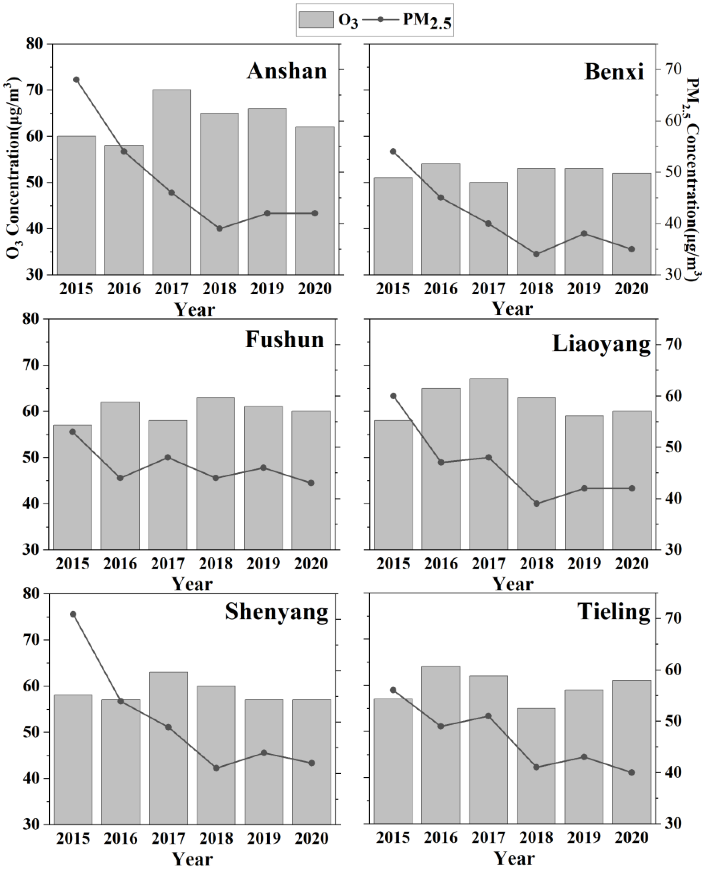
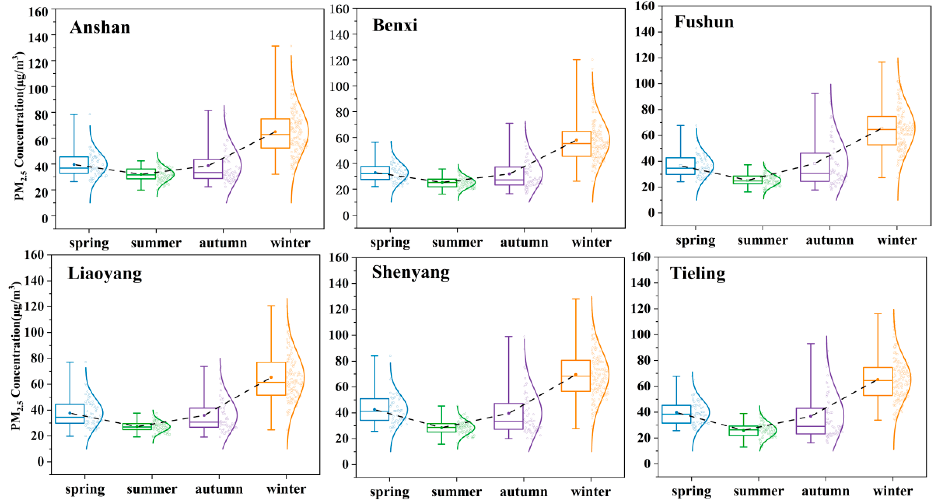
3.1. Temporal Variation

The annual average concentrations and change trends of PM2.5 and O3 in six cities of CLUA are investigated as shown in Figure 2. PM2.5 basically showed a trend of declining from 2015 to 2020. The average concentration of PM2.5 in Fushun decreased by 18% from 2015 to 2016, and increased slightly in 2017 and 2019, but was still lower than 53 µg/m3 in 2015. China began to implement the environmental protection tax law in 2018 to strengthen the management of air pollution punishment, which explains why the PM2.5 concentration in each city was the lowest in 2018. In addition, straw burning was prohibited in the study area, and Liaoning Province began to completely ban small coal-fired boilers of 10 tons and below in 2016 to improve air quality. The average concentration of PM2.5 in Anshan City decreased from 67 µg/m3 to 41.6 µg/m3, which was 66.4% lower in 2020 than in 2015. In 2020, the lowest PM2.5 value appeared in Benxi City, which was 34.7 µg/m3. Except for Benxi, PM2.5 in other cities (Anshan, Fushun, Liaoyang, Shenyang, Tieling) did not meet China Class II Environmental Air Quality Standard (CAAQS) limited to 35 µg/m3. This shows that the government needs to strengthen particulate matter control in these cities. Unlike PM2.5, the annual average concentration of ozone does not change much in various regions, and the trend of change is slightly different. This can be attributed to the fact that ozone is affected by more meteorological conditions and chemical reactions [36,37], so its regional characteristics are less obvious. The average concentration of O3 in Shenyang increased from 2015 to 2017 and decreased significantly after reaching peak value in 2017. Among them, the ozone concentration in Anshan, Liaoyang, and Shenyang reached the peak concentrations in 2017, which were 68.76 µg/m3, 66.27 µg/m3, and 63.46 µg/m3 respectively.
Figure 3 shows the monthly variation of the 24-h multi-year average concentration of PM2.5 in CLUA from 2015 to 2020. It can be found that PM2.5 pollution is the most serious at the beginning and the end of the year (January to March and October to December), and the PM2.5 pollution is lower from May to September. In Northeast China, there is a large area of open burning of crop residues, which is one of the reasons for PM2.5 pollution in autumn and winter. In addition, PM2.5 pollution peaked in the heating period. Due to the long heating period, PM2.5 pollution continued until the next spring. It can be seen that the frequency of low PM2.5 concentration in Benxi area is higher, which also indicates that the PM2.5 pollution in Benxi is relatively lower than in other areas, because Benxi is rainy in summer and autumn, and the wind direction is southeast, which is conducive to the diffusion of pollutants. In general, the PM2.5 concentration in several cities resulted in high values at night and low values during the day. In this latter case, low-concentration PM2.5 were registered from 14:00 to 17:00, while the peak of PM2.5 mainly were registered from 7:00 to 9:00 and from 18:00 to 23:00. The first peak is related to atmospheric stability and the increase of human activities during this period [38]. This can be attributed to the intensification of atmospheric turbulence and the gradual decrease of PM2.5 concentration with the increase of temperature in the morning. The evening peak in the cities appears after sunset, so the PM2.5 emission increases. In addition, the surface radiation cooling reduces the height of the boundary layer, and the atmosphere tends to be stable, leading PM2.5 concentration to continue to rise [39].
Figure 4 and Figure 5 are box charts of daily average concentrations of PM2.5 and O3 in different seasons in CLUA from 2015 to 2020 respectively. The upper and lower frames of the box represent 75% and 25% quantiles respectively. The data points next to the box in the figures correspond to the daily average concentration of pollutants, and a normal distribution curve is added according to the concentration value. It is obvious that PM2.5 pollution trends are the same in all cities. PM2.5 pollution is the most serious in winter, followed by spring and autumn, and significantly lower in summer than in other seasons. In summer, the concentration of PM2.5 in the Anshan area is the highest, 32.02 µg/m3 (<35 µg/m3). However, the concentration of PM2.5 in other cities does not exceed 30 µg/m3. It may be related to the fact that Anshan is a heavy industrial city and the main pollution source is a fixed source. Compared with other seasons, the rainy weather in summer has an obvious effect on the wet deposition of pollutants, so the PM2.5 concentration is relatively lower [40]. In spring and autumn, PM2.5 pollution is the most serious in Shenyang, followed by Tieling and Anshan. The concentration of PM2.5 in Benxi is the lowest. In winter, PM2.5 pollution in Shenyang is the most serious (69.57 µg/m3), which is 2.46 times higher than that in summer. The concentration of PM2.5 in Benxi City is the lowest, 57.9 µg/m3. This is consistent with other results obtained using MODIS inversion data [41,42]. The high concentration in winter is mainly due to the high population density in the built-up area and the low temperature in winter in the north, so the amount of coal combustion increases. In addition, inversion is more likely to occur in winter, which is not conducive to the diffusion of pollutants [43,44].
Being affected by the seasonal variation of meteorological conditions, the ozone concentration is opposite to that of PM2.5. In spring and summer, it is significantly higher than that in autumn and winter. The seasonal pattern of ozone in central Liaoning urban agglomeration is the same as that in other regions, with the overall pattern as summer > spring > autumn > winter [45,46,47]. In summer, the O3 concentration in Shenyang is 131.14 µg/m3, and the O3 concentration in Benxi is 95.3 µg/m3. Some studies have shown that direct emission of surface ozone is different from that of other air pollutants. O3 is mainly generated by nitrogen oxides (NOx) and volatile organic compounds (VOCs) through a series of complex photochemical reactions [48,49]. The high temperature and high chemical reaction rate in spring and summer make the ozone concentration much higher than that in other seasons. In addition, Benxi is different from other regions, and ozone concentration in summer is lower than that in spring. The ozone concentration in Fushun is higher in six cities. Huang et al. mentioned that there is intercity pollution between Fushun and Shenyang. Therefore, the ozone concentration in the monitoring stations near Shenyang is higher (Figure 6).

3.2. Spatial Analysis

The spatial sites distribution of O3 and PM2.5 in CLUA is shown in Figure 6 and Figure 7. PM2.5 and O3 of all monitoring stations in Shenyang showed an obvious downward trend from 2015 to 2020. In 2015, the high concentrations of PM2.5 were mainly located in LD, TY, SLX in Shenyang, TD, and TSS in Anshan. On the whole, since 2016, the concentration values of monitoring stations near the junction of Shenyang and Fushun have been higher. The stations with high concentrations of PM2.5 are mainly concentrated in Shenyang urban areas, TD, SF, and WH. These stations are mostly concentrated in urban areas with high population, which leads to a higher concentration of pollutants caused by motor vehicles and industrial discharge.
The spatial distribution trend of ozone is basically the opposite of PM2.5. The concentration of O3 in rural areas is higher, such as XT, DY, DM, HW, and JSJ, etc. As a secondary pollutant, the formation of surface ozone is mainly related to its precursors (NOx and VOCs). The source analysis of atmospheric VOCs in some areas shows that the contribution rate of motor vehicle sources is high, which is the main source of urban atmospheric VOCs [50,51]. The ozone pollution occurring in the urban areas is transported to the suburbs with certain meteorological conditions [52]. The higher vegetation coverage is conducive to photochemical reaction, resulting in higher ozone concentration in the suburbs [53]. In addition, it can be found that the O3 concentration is higher at the stations near the junction of Liaoyang and Anshan. From 2015 to 2020, the O3 concentration in western cities are lower than that in eastern cities. The high ozone concentration is distributed in a belt from Anshan, Liaoyang and Shenyang to Tieling and Fushun in the northeast. While the ozone concentration of Benxi in the east is always low, which is consistent with the results in Figure 2. Figure 8 shows that the ozone concentration in CLUA increased significantly from 2015 to 2017, and began to decrease gradually in 2018. It shows that while dealing with climate change, controlling pollutant emission reduction plays an active role in ozone mass concentration control.

3.3. Transmission Path Characteristics in Shenyang Region

As the Shenyang area is the geographical and economic center of CLUA, its PM2.5 and O3 pollution is severe. Therefore, this study selects Shenyang city for backward trajectory cluster analysis and potential source area analysis. Cluster analysis of the backward airflow trajectories transported to Shenyang at 0:00, 6:00, 12:00, and 18:00 every day from 2015 to 2020 (Figure 9). There are six categories of backward trajectories in spring. The air flows in spring are mainly south (trajectory 1 and trajectory 5) and northwest (trajectory 3 and trajectory 6), which account for 67.79% of the airflows in spring. There are four categories of backward trajectories in summer. In summer, affected by the marine airflows, the southerly airflows (trajectory 1) and southeast airflows (trajectory 4) are predominant, accounting for 68.43% of the airflows in summer. There are seven categories of backward trajectories in autumn and six categories of backward trajectories in winter. In autumn and winter, the airflows are mostly northwest and the transmission distance is longer with faster speed, which may be related to the propagation of the East Asian winter monsoon. Except in summer, the airflows from the Beijing-Tianjin-Hebei region have all turned back significantly.
Based on the cluster analysis results of airflow backward trajectories in each season, the PM2.5 and ozone concentration data in Shenyang are combined (Table 2) to quantitatively analyze the impact of various trajectories on PM2.5 and ozone in Shenyang.
Consistent with the results discussed above, the PM2.5 concentration corresponding to each air flow in autumn and winter is higher than that in spring and summer. In winter, the PM2.5 concentration corresponding to the airflow (trajectory 3) from the junction of Liaoning and Hebei, Bohai Bay and southwest Liaoning is the highest, 106.02 µg/m3. The second is the air flow from Northeast Inner Mongolia, northwest Jilin and northeast Liaoning (trajectory 6), and the corresponding PM2.5 concentration is 105.23 µg/m3. The corresponding concentration of ozone in the southerly flow (trajectory 1) from the Yellow Sea in spring is 142.41 µg/m3, followed by the air flow (trajectory 5) is 136.5 µg/m3.
The long-distance transport of northwest air flow from Hunshandak Sandy Land in Northwest Inner Mongolia and the Gobi Desert in central Mongolia is the main transport path affecting the PM2.5 concentration in Shenyang in four seasons. In addition, southwest air flows through densely populated areas such as Beijing, Tianjin, and Hebei. The Bohai Sea has heavy shipping emissions, making it another main transmission path affecting PM2.5 pollution in Shenyang.

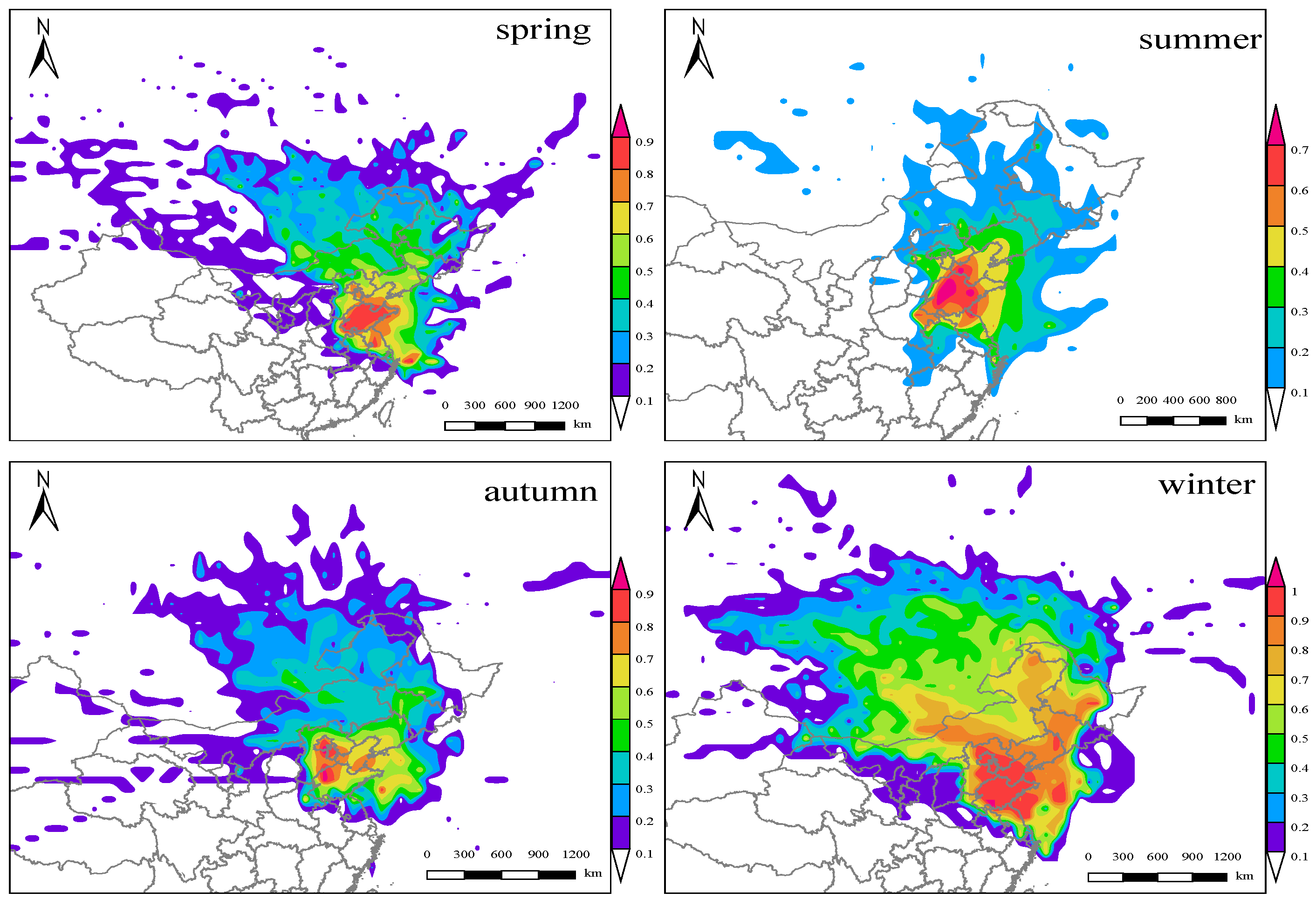
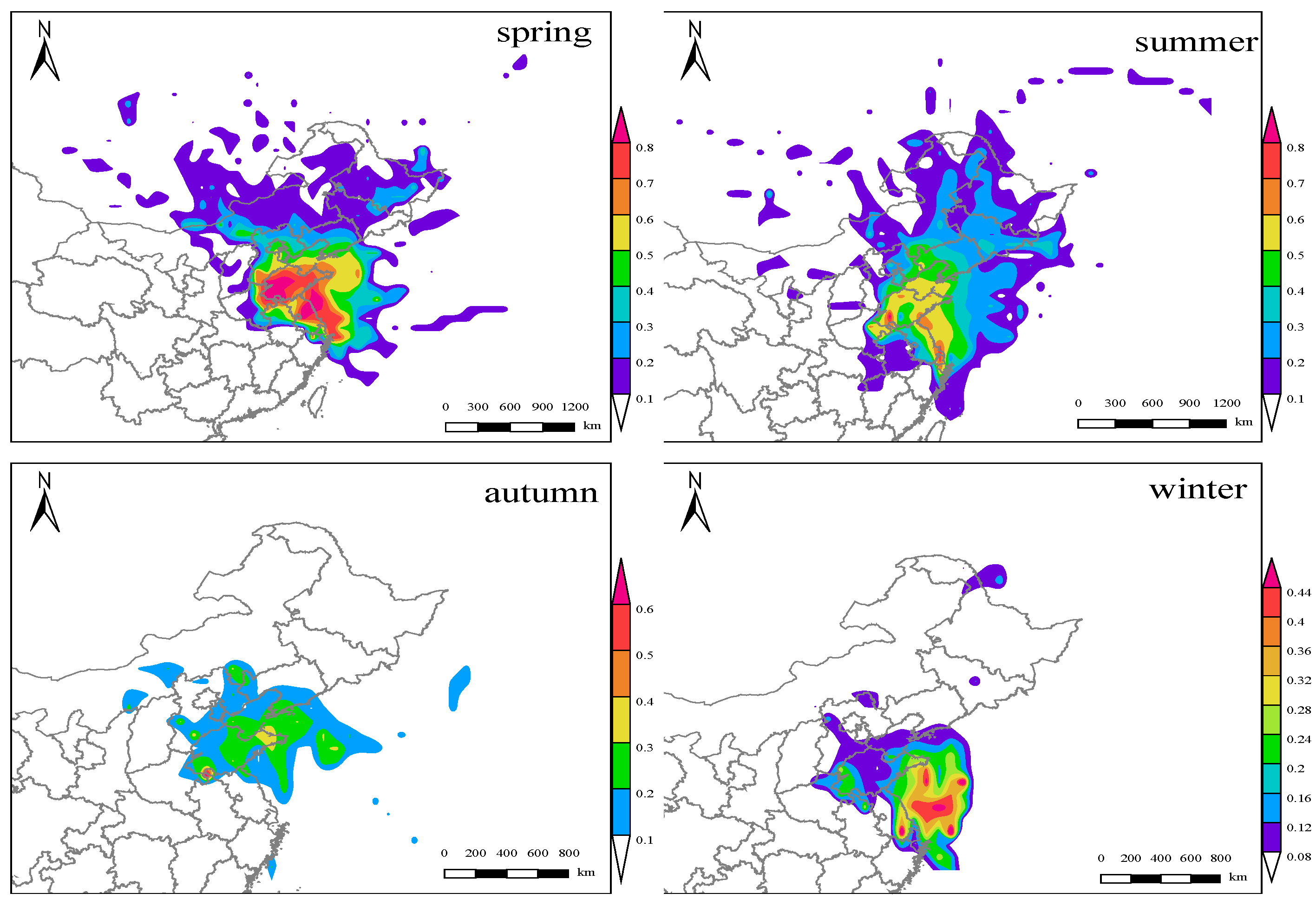
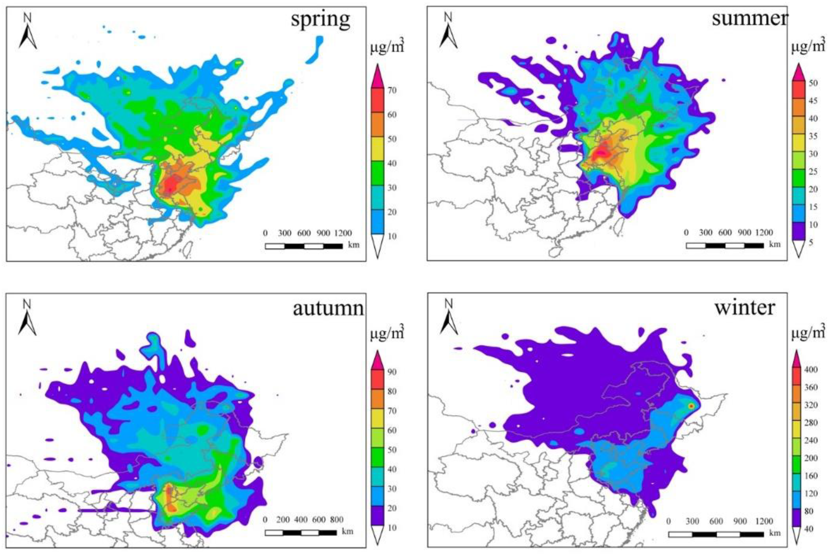
3.4. Characteristics of Potential Source Areas in Shenyang

We conduct the potential source contribution factor (WPSCF) analysis and the concentration weight trajectory (WCWT) analysis based on the backward trajectory of each season in Shenyang from 2015 to 2020, in order to fully reflect the long-term impact characteristics and contribution of potential source regions on the mass concentration of PM2.5 and O3 in Shenyang. The results are shown in Figure 10, Figure 11, Figure 12 and Figure 13. The larger the calculated value of WPSCF, the greater the impact of the area on the mass concentration of PM2.5 and O3 in Shenyang. The higher value of WCWT, the greater the contribution of the grid area to the pollution of PM2.5 and O3 in Shenyang.
The WPSCF value of PM2.5 is the lowest in summer, and it can be found that WPSCF and WCWT have consistent spatial distribution characteristics in central Shandong. It can be seen that the regions with a higher contribution to the PM2.5 concentration in Shenyang in spring were concentrated in the central Shandong Province and the northwestern parts of Jiangsu Province, with WPSCF value higher than 0.7 and corresponding WCWT value higher than 50 µg/m3 (Figure 10 and Figure 12). In summer, WPSCF value is higher near Zaozhuang and Jinan in Shandong Province, and WCWT value is 45~50 µg/m3. The regions with relatively high WPSCF in autumn are mainly concentrated in Beijing-Tianjin-Hebei Urban Agglomeration and northwestern part of the Shandong Province, and the WCWT value is higher than 80 µg/m3. In winter, due to the heavy PM2.5 pollution, the WPSCF value of PM2.5 is high and wide, indicating that the PM2.5 pollution in Shenyang has certain regional characteristics. The high value of WPSCF mainly occurs in Beijing Tianjin Hebei Urban Agglomeration, Bohai Sea area, Lianyungang City, Shandong Province and Jiangsu Province, the northeast of Liaoning, the middle of Jilin, and the middle of Heilongjiang, showing a wide coverage of northeast trending potential contribution source zone (WPSCF > 0.8). It is worth noting that in the WCWT distribution, the central Heilongjiang shows more than 240 PM2.5. It also mentioned that in winter, Liaoning Province is subject to long-distance transportation from Heilongjiang Province, resulting in serious haze pollution [54].
It can be seen from Figure 11 that there are many regions with higher contributions of the O3 concentration in Shenyang in spring and summer. They are mainly concentrated in Bohai Bay, Shandong Province, Jiangsu Province, and the nearby Yellow Sea. The WPSCF value is higher than 0.6 and the corresponding WCWT value is more than 110 µg/m3. Among them, Jiangsu Province is an economically developed region in China, with intensive secondary industry and serious pollutant emission. The high WPSCF values in the Bohai Sea and the Yellow Sea may be the pollutants in their adjacent areas and are transmitted to the nearby sea areas through the sea land winds. Then they are transported to the northeast along the Bohai Bay and the Yellow Sea bay, sinking in Shenyang. However, as mentioned above, compared with PM2.5, ozone is unstable and the formation conditions are complex, so it is more difficult to determine the potential source area of ozone. PSCF and CWT methods show that the high ozone content in Shenyang mainly comes from the transmission in the Yellow Sea, Bohai Sea, and its adjacent areas.
Combined with the analysis of PSCF and CWT, it can be found that the main potential sources areas affecting the PM2.5 mass concentration of in Shenyang in autumn and winter are Beijing-Tianjin-Hebei Urban Agglomeration, Shandong Province, Jiangsu Province, and nearby sea areas. This shows that the atmospheric circulation has an important impact on the regional transmission of the city. In addition, the main potential source areas of O3 mass concentration in spring and summer are coastal cities and the Bohai Sea and Yellow Sea. This is also consistent with the backward air flow trajectory with heavy pollution in each season, and the influence of long-distance transmission of pollution concentration is small. Through potential source analysis, we should pay attention to the industrial source supply in the surrounding areas of cities and the marine source provided by marine pollution, and strengthen joint prevention and control of air pollution among regions.

4. Conclusions

The PM2.5 concentration has fluctuated from 2016 to 2020 in Fushun, and has declined year by year from 2015 to 2020 in other areas of the CLUA. The lowest PM2.5 level occurred in 2018. Except for Benxi, PM2.5 in other cities (Anshan, Fushun, Liaoyang, Shenyang, Tieling) did not meet the China Class II Environmental Air Quality Standard (CAAQS) limit of 35 µg/m3. The annual mean concentration of ozone has little change in different regions, and the variation trend is different. The ozone concentration in Anshan, Liaoyang, and Shenyang reached the peak value in 2017, which was 68.76 µg/m3, 66.27 µg/m3, and 63.46 µg/m3, respectively. PM2.5 pollution is the most severe at the beginning and the end of each year (January to March and October to December). The concentration of PM2.5 in all cities showed the characteristics of high at night and low during the day. Affected by human activities and atmospheric movements, there are two peaks at 7:00~9:00 and 18:00~23:00. The seasonal pattern of PM2.5 concentration was winter > spring > autumn > summer. In winter, PM2.5 pollution in Shenyang is 69.57 µg/m3, which is 2.46 times of that in summer. The seasonal pattern of ozone concentration is summer > spring > autumn > winter. In summer, The O3 concentration in Shenyang is the highest, 131.14 µg/m3, 1.37 times of that in Benxi. The ozone concentration in Fushun area is affected by the intercity pollution in Shenyang.
In terms of the spatial distribution of PM2.5 and O3 concentrations, the concentrations of PM2.5 in the western cities (Shenyang, Liaoyang, and Anshan) present higher than that in the eastern ones (Tieling, Fushun, and Benxi), and the higher values are concentrated in urban monitoring stations. On the contrary, the concentration of O3 is higher in rural areas, which is related to its precursors. The high concentration of ozone in Anshan, Liaoyang, and Shenyang extends to Tieling and Fushun in the northeast. The ozone concentration of Benxi city in the east is always low. Moreover, the ozone concentration in the central Liaoning urban agglomeration began to decrease gradually in 2018.
Through backward trajectory cluster analysis, it is found that the main transmission paths affecting Shenyang are southerly short-distance and northwest long-distance airflows in spring, southerly short-distance airflow in summer, southerly and northerly airflows in autumn, and northwestern long-distance airflow in winter. In winter, southwest airflows and northeast airflows have the highest PM2.5 concentration, which is 106.02 µg/m3 and 105.23 µg/m3 respectively. The ozone concentration corresponding to the southerly airflows in spring and summer is the highest, which is 142.41 µg/m3 and 139.83 µg/m3, respectively.
Through the WPSCF and WCWT analysis, it is found that the main potential source areas affecting the mass concentration of PM2.5 in Shenyang in autumn and winter are Beijing-Tianjin-Hebei urban agglomeration, Shandong Province, Jiangsu Province, and nearby sea areas, showing a potential contribution source belt with a wide coverage of northeast trend. In addition, the main potential source areas of ozone mass concentration in spring and summer are mainly coastal cities and the Bohai sea and Yellow Sea. Through the analysis of potential sources, we should pay attention to the industrial source supply in the surrounding areas and the marine source provided by marine pollution. We will strengthen joint prevention and control of air pollution between regions.

Author Contributions

Conceptualization, Y.Z.; methodology, J.W.; software, Y.Z.; validation, J.W. and C.F.; formal analysis, Z.L.; investigation, Y.Z.; resources, C.F.; data curation, C.F.; writing—original draft preparation, Y.Z.; writing—review and editing, J.W., Y.Z. and C.F.; visualization, C.F.; supervision, C.F.; project administration, J.W. and C.F. All authors have read and agreed to the published version of the manuscript.

Funding

This research received no external funding.

Acknowledgments

The authors would like to thank the group members of Laboratory 537 and 142 of Jilin University.

Conflicts of Interest

The authors declare no conflict of interest.

References

  1. Yang, B.Y.; Qian, Z.; Li, S.; Markevych, I.; Bloom, M.S. Ambient air pollution in relation to diabetes and glucose-homoeostasis markers in China: A cross-sectional study with findings from the 33 Communities Chinese Health Study. Lancet Planet. Health 2018, 2, e113. [Google Scholar] [CrossRef] [Green Version]
  2. Xia, S.Y.; Huang, D.S.; Jia, H.; Zhao, Y.; Li, N.; Mao, M.Q.; Lin, H.; Li, Y.X.; He, W.; Zhao, L. Relationship between atmospheric pollutants and risk of death caused by cardiovascular and respiratory diseases and malignant tumors in Shenyang, China, from 2013 to 2016: An ecological research. Chin. Med. J. 2019, 132, 2269–2277. [Google Scholar] [CrossRef] [PubMed]
  3. Lei, R.Q.; Zhu, F.R.; Cheng, H.; Liu, J.; Shen, C.W.; Zhang, C.; Xu, Y.C.; Xiao, C.C.; Li, X.R.; Zhang, J.Q.; et al. Short-term effect of PM2.5/O-3 on non-accidental and respiratory deaths in highly polluted area of China. Atmos. Pollut. Res. 2019, 10, 1412–1419. [Google Scholar] [CrossRef]
  4. Guan, Y.; Xiao, Y.; Wang, Y.M.; Zhang, N.N.; Chu, C.J. Assessing the health impacts attributable to PM2.5 and ozone pollution in 338 Chinese cities from 2015 to 2020. Environ. Pollut. 2021, 287, 117623. [Google Scholar] [CrossRef]
  5. Dong, D.X.; Xu, B.Y.; Shen, N.; He, Q. The adverse impact of air pollution on China’s economic growth. Sustainability 2021, 13, 9056. [Google Scholar] [CrossRef]
  6. Wu, Z.Y.; Zhang, Y.Q.; Zhang, L.M.; Huang, M.J.; Zhong, L.J.; Chen, D.H.; Wang, X.M. Trends of outdoor air pollution and the impact on premature mortality in the Pearl River Delta region of southern China during 2006–2015. Sci. Total Environ. 2019, 690, 248–260. [Google Scholar] [CrossRef] [PubMed]
  7. Zhang, N.N.; Ma, F.; Qin, C.B.; Li, Y.F. Spatiotemporal trends in PM2.5 levels from 2013 to 2017 and regional demarcations for joint prevention and control of atmospheric pollution in China. Chemosphere 2018, 210, 1176–1184. [Google Scholar] [CrossRef] [PubMed]
  8. Chen, Z.; Wang, J.N.; Ma, G.X.; Zhang, Y.S. China tackles the health effects of air pollution. Lancet 2013, 382, 1959–1960. [Google Scholar] [CrossRef]
  9. Guo, H.; Cheng, T.H.; Gu, X.F.; Wang, Y.; Chen, H.; Bao, F.W.; Shi, S.Y.; Xu, B.R.; Wang, W.N.; Zuo, X.; et al. Assessment of PM2.5 concentrations and exposure throughout China using ground observations. Sci. Total Environ. 2017, 601, 1024–1030. [Google Scholar] [CrossRef]
  10. Liaoning Provincial Environmental Protection Bureau. Bulletin on the Ecological Environment of Liaoning Province in 2020; Liaoning Provincial Environmental Protection Bureau: Shenyang, China, 2020.
  11. Liu, S.C.; Xing, J.; Wang, S.X.; Ding, D.A.; Chen, L.; Hao, J.M. Revealing the impacts of transboundary pollution on PM2.5-related deaths in China. Environ. Int. 2020, 134, 105323. [Google Scholar] [CrossRef]
  12. Li, X.L.; Hu, X.M.; Shi, S.Y.; Shen, L.D.; Luan, L.; Ma, Y.J. Spatiotemporal variations and regional transport of air pollutants in two urban agglomerations in northeast China plain. Chin. Geogr. Sci. 2019, 29, 917–933. [Google Scholar] [CrossRef] [Green Version]
  13. Nan, Y.; Zhang, Q.Q.; Zhang, B.H. Analysis on the influencing factors of long-term change of grid PM2.5 in typical regions of China based on gam model. Environ. Sci. 2020, 41, 499–509. [Google Scholar]
  14. Chen, W.W.; Zhang, S.C.; Tong, Q.S.; Zhang, X.L.; Zhao, H.M.; Ma, S.Q.; Xiu, A.J.; He, Y.X. Regional characteristics and causes of haze events in Northeast China. Chin. Geogr. Sci. 2018, 28, 836–850. [Google Scholar] [CrossRef] [Green Version]
  15. Gao, C.; Xiu, A.; Zhang, X.; Chen, W.; Liu, Y.; Zhao, H.; Zhang, S. Spatiotemporal characteristics of ozone pollution and policy implications in Northeast China. Atmos. Pollut. Res. 2020, 11, 357–369. [Google Scholar] [CrossRef]
  16. Liang, Z.H.; Ju, T.Z.; Dong, H.P.; Geng, T.Y.; Duan, J.L.; Huang, R.R. Study on the variation characteristics of tropospheric ozone in Northeast China. Environ. Monit. Assess. 2021, 193, 282. [Google Scholar] [CrossRef] [PubMed]
  17. Wang, H.; Ding, K.; Huang, X.; Wang, W.; Ding, A. Insight into ozone profile climatology over northeast China from aircraft measurement and numerical simulation. Sci. Total Environ. 2021, 785, 147308. [Google Scholar] [CrossRef]
  18. Luo, M.; Ji, Y.Y.; Ren, Y.Q.; Gao, F.H.; Zhang, H.; Zhang, L.H.; Yu, Y.Q.; Li, H. Characteristics and health risk assessment of PM2.5-Bound PAHs during heavy air pollution episodes in winter in urban area of Beijing, China. Atmosphere 2021, 12, 323. [Google Scholar] [CrossRef]
  19. Li, B.; Shi, X.F.; Liu, Y.P.; Lu, L.; Wang, G.L.; Thapa, S.; Sun, X.Z.; Fu, D.L.; Wang, K.; Qi, H. Long-term characteristics of criteria air pollutants in megacities of Harbin-Changchun megalopolis, Northeast China: Spatiotemporal variations, source analysis, and meteorological effects. Environ. Pollut. 2020, 267, 10. [Google Scholar] [CrossRef] [PubMed]
  20. Dai, H.B.; Zhu, J.; Liao, H.; Li, J.D.; Liang, M.X.; Yang, Y.; Yue, X. Co-occurrence of ozone and PM2.5 pollution in the Yangtze River Delta over 2013–2019: Spatiotemporal distribution and meteorological conditions. Atmos. Res. 2021, 249, 9. [Google Scholar] [CrossRef]
  21. Wang, Y.Q.; Zhang, X.Y.; Draxler, R.R. TrajStat: GIS-based software that uses various trajectory statistical analysis methods to identify potential sources from long-term air pollution measurement data. Environ. Model. Softw. 2009, 24, 938–939. [Google Scholar] [CrossRef]
  22. Wang, X.Q.; Zhang, T.S.; Xiang, Y.; Lv, L.H.; Fan, G.Q.; Ou, J.P. Investigation of atmospheric ozone during summer and autumn in Guangdong Province with a lidar network. Sci. Total Environ. 2021, 751, 141740. [Google Scholar] [CrossRef]
  23. Stein, A.F.; Draxler, R.R.; Rolph, G.D.; Stunder, B.J.B.; Cohen, M.D.; Ngan, F. Noaa’s hysplit atmospheric transport and dispersion modeling system. bull. Amer. Meteorol. Soc. 2015, 96, 2059–2077. [Google Scholar] [CrossRef]
  24. Stohl, A.; Forster, C.; Frank, A.; Seibert, P.; Wotawa, G. Technical note: The Lagrangian particle dispersion model FLEXPART version 6.2. Atmos. Chem. Phys. 2005, 5, 2461–2474. [Google Scholar] [CrossRef] [Green Version]
  25. Zhang, Y.R.; Zhang, H.L.; Deng, J.J.; Du, W.J.; Hong, Y.W.; Xu, L.L.; Qiu, Y.Q.; Hong, Z.Y.; Wu, X.; Ma, Q.L.; et al. Source regions and transport pathways of PM2.5 at a regional background site in East China. Atmos. Environ. 2017, 167, 202–211. [Google Scholar] [CrossRef] [Green Version]
  26. Cesari, R.; Paradisi, P.; Allegrini, P. Source identification by a statistical analysis of backward trajectories based on peak pollution events. Int. J. Environ. Pollut. 2014, 55, 94–103. [Google Scholar] [CrossRef]
  27. Sparks, D.N. Euclidean cluster analysis. R. Stat. Soc. Ser. C Appl. Stat. 1973, 22, 126–130. [Google Scholar] [CrossRef]
  28. Hong, Q.Q.; Liu, C.; Hu, Q.H.; Xing, C.Z.; Tan, W.; Liu, H.R.; Huang, Y.; Zhu, Y.; Zhang, J.S.; Geng, T.Z.; et al. Evolution of the vertical structure of air pollutants during winter heavy pollution episodes: The role of regional transport and potential sources. Atmos. Res. 2019, 228, 206–222. [Google Scholar] [CrossRef]
  29. Zhang, Z.Y.; Wong, M.S.; Lee, K.H. Estimation of potential source regions of PM2.5 in Beijing using backward trajectories. Atmos. Pollut. Res. 2015, 6, 173–177. [Google Scholar] [CrossRef] [Green Version]
  30. Ashbaugh, L.L.; Malm, W.C.; Sadeh, W.Z. A residence time probability analysis of sulfur concentrations at grand Canyon National Park. Atmos. Environ. 1985, 19, 1263–1270. [Google Scholar] [CrossRef]
  31. Hsu, Y.K.; Holsen, T.M.; Hopke, P.K. Locating and quantifying PCB sources in Chicago: Receptor modeling and field sampling. Environ. Sci. Technol. 2003, 37, 681–690. [Google Scholar] [CrossRef] [PubMed]
  32. Wang, Y.Q.; Zhang, X.Y.; Arimoto, R. The contribution from distant dust sources to the atmospheric particulate matter loadings at XiAn, China during spring. Sci. Total Environ. 2006, 368, 875–883. [Google Scholar] [CrossRef]
  33. Jeong, U.; Kim, J.; Lee, H.; Jung, J.; Kim, Y.J.; Song, C.H.; Koo, J.H. Estimation of the contributions of long range transported aerosol in East Asia to carbonaceous aerosol and PM concentrations in Seoul, Korea using highly time resolved measurements: A PSCF model approach. J. Environ. Monit. 2011, 13, 1905–1918. [Google Scholar] [CrossRef]
  34. Kabashnikov, V.P.; Chaikovsky, A.P.; Kucsera, T.L.; Metelskaya, N.S. Estimated accuracy of three common trajectory statistical methods. Atmos. Environ. 2011, 45, 5425–5430. [Google Scholar] [CrossRef]
  35. Dimitriou, K. The dependence of PM size distribution from meteorology and local-regional contributions, in Valencia (Spain)—A CWT model approach. Aerosol Air Qual. Res. 2015, 15, 1979–1989. [Google Scholar] [CrossRef]
  36. Zhang, Y.; Wang, W.; Wu, S.Y.; Wang, K.; Minoura, H.; Wang, Z.F. Impacts of updated emission inventories on source apportionment of fine particle and ozone over the southeastern US. Atmos. Environ. 2014, 88, 133–154. [Google Scholar] [CrossRef]
  37. Otero, N.; Sillmann, J.; Schnell, J.L.; Rust, H.W.; Butler, T. Synoptic and meteorological drivers of extreme ozone concentrations over Europe. Environ. Res. Lett. 2016, 11, 13. [Google Scholar] [CrossRef]
  38. Fan, H.; Zhao, C.F.; Yang, Y.K.; Yang, X.C. Spatio-temporal variations of the PM2.5/PM10 ratios and its application to air pollution type classification in China. Front. Environ. Sci. 2021, 9, 281. [Google Scholar] [CrossRef]
  39. Pan, L.; Xu, J.M.; Tie, X.X.; Mao, X.Q.; Gao, W.; Chang, L.Y. Long-term measurements of planetary boundary layer height and interactions with PM2.5 in Shanghai, China. Atmos. Pollut. Res. 2019, 10, 989–996. [Google Scholar] [CrossRef]
  40. Chen, Z.; Chen, D.; Zhao, C.; Kwan, M.P.; Cai, J.; Zhuang, Y.; Zhao, B.; Wang, X.; Chen, B.; Yang, J.; et al. Influence of meteorological conditions on PM2.5 concentrations across China: A review of methodology and mechanism. Environ. Int. 2020, 139, 105558. [Google Scholar] [CrossRef] [PubMed]
  41. Zhao, H.; Che, H.; Zhang, X.; Ma, Y.; Wang, Y.; Wang, X.; Liu, C.; Hou, B.; Che, H. Aerosol optical properties over urban and industrial region of Northeast China by using ground-based sun-photometer measurement. Atmos. Environ. 2013, 75, 270–278. [Google Scholar] [CrossRef]
  42. Zhao, H.; Gui, K.; Ma, Y.; Wang, Y.; Wang, Y.; Wang, H.; Zheng, Y.; Li, L.; Zhang, L.; Che, H.; et al. Climatological variations in aerosol optical depth and aerosol type identification in Liaoning of Northeast China based on MODIS data from 2002 to 2019. Sci. Total Environ. 2021, 781, 146810. [Google Scholar] [CrossRef]
  43. Xu, Z.; Huang, X.; Nie, W.; Chi, X.; Xu, Z.; Zheng, L.; Sun, P.; Ding, A. Influence of synoptic condition and holiday effects on VOCs and ozone production in the Yangtze River Delta region, China. Atmos. Environ. 2017, 168, 112–124. [Google Scholar] [CrossRef]
  44. Chen, J.; Shen, H.; Li, T.; Peng, X.; Cheng, H.; Ma, A.C. Temporal and spatial features of the correlation between PM2.5 and O3 concentrations in China. Int, J. Environ. Res. Public Health 2019, 16, 4824. [Google Scholar] [CrossRef] [PubMed] [Green Version]
  45. Tui, Y.; Qiu, J.; Wang, J.; Fang, C. Analysis of spatio-temporal variation characteristics of main air pollutants in Shijiazhuang city. Sustainability 2021, 13, 941. [Google Scholar] [CrossRef]
  46. Chan, K.L.; Wang, S.S.; Liu, C.; Zhou, B.; Wenig, M.O.; Saiz-Lopez, A. On the summertime air quality and related photochemical processes in the megacity Shanghai, China. Sci. Total Environ. 2017, 580, 974–983. [Google Scholar] [CrossRef]
  47. Qian, Y.; Xu, B.; Xia, L.J.; Chen, Y.L.; Deng, L.C.; Wang, H.; Zhang, G. Characteristics of ozone pollution and relationships with meteorological factors in Jiangxi province. Environ. Sci. 2021, 42, 2190–2201. [Google Scholar] [CrossRef]
  48. Huang, D.; Li, Q.L.; Wang, X.X.; Li, G.X.; Sun, L.Q.; He, B.; Zhang, L.; Zhang, C.S. Characteristics and trends of ambient ozone and nitrogen oxides at urban, suburban, and rural sites from 2011 to 2017 in Shenzhen, China. Sustainability 2018, 10, 530. [Google Scholar] [CrossRef]
  49. Wang, T.; Xue, L.K.; Brimblecombe, P.; Lam, Y.F.; Li, L.; Zhang, L. Ozone pollution in China: A review of concentrations, meteorological influences, chemical precursors, and effects. Sci. Total Environ. 2017, 575, 1582–1596. [Google Scholar] [CrossRef]
  50. Gu, Y.; Liu, B.S.; Li, Y.F.; Zhang, Y.F.; Bi, X.H.; Wu, J.H.; Song, C.B.; Dai, Q.L.; Han, Y.; Ren, G.; et al. Multi-scale volatile organic compound (VOC) source apportionment in Tianjin, China, using a receptor model coupled with 1-hr resolution data. Environ. Pollut. 2020, 265, 23. [Google Scholar] [CrossRef]
  51. Li, C.; Liu, Y.; Cheng, B.; Zhang, Y.; Liu, X.; Qu, Y.; An, J.; Kong, L.; Zhang, Y.; Zhang, C.; et al. A comprehensive investigation on volatile organic compounds (VOCs) in 2018 in Beijing, China: Characteristics, sources and behaviours in response to O3 formation. Sci. Total Environ. 2022, 806, 150247. [Google Scholar] [CrossRef] [PubMed]
  52. Liu, H.; Zhang, M.; Han, X. A review of surface ozone source apportionment in China. Atmos. Ocean. Sci. Lett. 2020, 13, 470–484. [Google Scholar] [CrossRef]
  53. Zhang, H.; Qiu, Z.; Sun, D.; Wang, S.; He, Y. Seasonal and interannual variability of satellite-derived chlorophyll-a (2000–2012) in the Bohai Sea, China. Remote Sens. 2017, 9, 582. [Google Scholar] [CrossRef] [Green Version]
  54. Yin, S.; Wang, X.; Zhang, X.; Zhang, Z.; Xiao, Y.; Tani, H.; Sun, Z. Exploring the effects of crop residue burning on local haze pollution in Northeast China using ground and satellite data. Atmos. Environ. 2019, 199, 189–201. [Google Scholar] [CrossRef]
Figure 1. Air quality monitoring station in CLUA.
Sustainability 14 00511 g001
Figure 2. Inter-annual changes of PM2.5 and O3 years in CLUA from 2015 to 2020.
Sustainability 14 00511 g002
Figure 3. Hourly variation of multi-year average concentration of PM2.5 in different months in CLUA from 2015 to 2020.
Sustainability 14 00511 g003
Figure 4. Seasonal variation of PM2.5 in CLUA from 2015 to 2020.
Sustainability 14 00511 g004
Figure 5. Seasonal variation of O3 in CLUA from 2015 to 2020.
Sustainability 14 00511 g005
Figure 6. Spatial site distribution of annual average mass concentration of MDA8 O3 in CLUA PM2.5 annual average mass concentration of CLUA from 2015 to 2020(AS: Anshan; BX: Benxi; FS: Fushun; LY: Liaoyang; SY: Shenyang; TL: Tieling).
Sustainability 14 00511 g006
Figure 7. Spatial site distribution of PM2.5 annual average mass concentration in CLUA from 2015 to 2020 (AS: Anshan; BX: Benxi; FS: Fushun; LY: Liaoyang; SY: Shenyang; TL: Tieling).
Sustainability 14 00511 g007
Figure 8. Spatial distribution of annual average mass concentration of MDA8 O3 in CLUA from 2015 to 2020 (AS: Anshan; BX: Benxi; FS: Fushun; LY: Liaoyang; SY: Shenyang; TL: Tieling).
Sustainability 14 00511 g008
Figure 9. Clustering analysis of backward trajectories of each season in Shenyang from 2015 to 2020 (the trajectories are marked with number and frequency).
Sustainability 14 00511 g009
Figure 10. WPSCF distribution of PM2.5 in Shenyang from 2015 to 2020.
Sustainability 14 00511 g010
Figure 11. WPSCF distribution of O3 in Shenyang from 2015 to 2020.
Sustainability 14 00511 g011
Figure 12. WCWT distribution of PM2.5 in Shenyang from 2015 to 2020.
Sustainability 14 00511 g012
Figure 13. WCWT distribution of O3 in Shenyang from 2015 to 2020.
Sustainability 14 00511 g013
Table 1. The details of 38 air quality monitoring stations.
CitiesAir Quality Monitoring Sites
NameAbbr.Longitude (°E)Latitude (°N)
AnshanMingDa New DistrictMD123.128941.0228
QianShan MountainQS123.015641.0831
ShenGouSiSG123.04441.1196
TaiPingTP123.048541.1442
TieXi District Industrial ParkTD122.948141.0833
Tiexi Sandao StreetTSS122.964241.0971
TaiYang ChengTYC123.01141.0931
BenxiCai TunCT123.730841.3047
Da YuDY123.843641.3283
Dong MingDM123.766941.2864
Wei NingWN123.814241.3472
Xi LakeXL123.752841.3369
Xinli TunXT123.798941.2692
FushunDaHuoFang ReservoirDHF124.087841.8864
DongZhou DistrictDZ124.038341.8625
ShenFuXinChengSF123.711741.8417
ShunCheng DistrictAC123.916941.8828
WangHua DistrictWH123.8141.8469
XinFu DistrictXF123.941.8594
LiaoyangBinHe RoadBH123.176141.2736
HongWei DistrictHW123.241.1953
TieXi District industrial parkTXD123.141741.2894
XinHua YuanXY123.1541.2553
ShenyangCangHai RoadCH123.28441.7694
LingDong StreetLD123.42841.8472
DongLing RoadDL123.54241.8336
JingShen StreetJS123.378341.9228
TaiYuan StreetTY123.399741.7972
YuNong RoadYN123.595341.9086
WenHua RoadWH123.4141.765
XiaoHeYan RoadXHY123.47841.7775
SenLin RoadSL123.683641.9339
Eastern of HunNan RoadHN123.53541.7561
ShenLiaoXi RoadSLX123.244441.7347
TielingWestern of HuiGong StreetHG123.813942.3022
Northern of JinShaJiang RoadJSJ123.715342.2217
ShuiShang ParkSP123.846942.292
Eastern of YinZhou RoadYZE123.848942.2864
Table 2. Statistical results of the mass concentration of all kinds of air flow in the four seasons of Shenyang.
SeasonAir Mass TypePM2.5StdevNumberOzoneStdevNumber
spring160.5124.70202142.4132.84189
260.6428.5965111.467.5714
359.2523.82100118.8715.4526
469.0034.10124128.9521.4150
567.1328.36138136.5026.83114
668.0131.7179126.3920.5131
summer150.1313.82286137.5831.06301
248.5611.9387126.9421.51113
358.1923.819125.6622.248
449.3213.65224139.8332.71230
autumn172.5938.98144119.9615.7811
257.6720.1376126.9719.325
370.9130.63117127.9120.7437
472.2159.5593113.8413.106
563.6548.37220.000.000
658.0420.425125.800.001
759.2525.67150121.2921.5944
winter178.5257.48543112.4115.374
290.2465.41506109.515.9610
3106.0285.85614114.8411.1216
466.1533.99450.000.000
576.4541.05222111.225.834
6105.2354.45489120.4919.1950
Publisher’s Note: MDPI stays neutral with regard to jurisdictional claims in published maps and institutional affiliations.

