Article

Path Planning for Autonomous Platoon Formation

by
Ouafae El Ganaoui-Mourlan
1,*,
Stephane Camp
2,
Thomas Hannagan
3,
Vaibhav Arora
2,
Martin De Neuville
2 and
Vaios Andreas Kousournas
2
1
IFP Energies Nouvelles, 1 et 4 Avenue de Bois-Préau, 92852 Rueil-Malmaison, France
2
IFP School, 228-232, Avenue Napoléon Bonaparte, CEDEX, 92852 Rueil-Malmaison, France
3
STELLANTIS, Centre Technique Vélizy, 78140 Vélizy-Villacoublay, France
*
Author to whom correspondence should be addressed.
Sustainability 2021, 13(9), 4668; https://doi.org/10.3390/su13094668
Submission received: 29 January 2021 / Revised: 1 April 2021 / Accepted: 15 April 2021 / Published: 22 April 2021
(This article belongs to the Special Issue Autonomous Vehicles: Future of Transportation Sustainability)

Abstract

:
In the context of automated highway systems (AHS), this work proposes an approach that enables a vehicle to autonomously join a platoon with optimized trajectory in the presence of dynamical traffic obstacles. A notable aspect is the use of Model Predictive Control (MPC) optimization of the planned path, in conjunction with a variant of the Rapidly-exploring Random Trees (RRT*) algorithm for the purpose of platoon formation. This combination efficiently explores the space of possible trajectories, returning trajectories that are smoothened out with respect to the dynamic constraints of the vehicle, while at the same time allowing for real-time implementation. The implementation we propose takes into consideration both localization and mapping through relevant sensors and V2V communication. The complete algorithm is tested over various nominal and worst-case scenarios, qualifying the merits of the proposed methodology.

1. Introduction

Energy consumption related to transport, combined with air quality issues, continues to attract the attention of scientists. Various emerging technologies have been proposed and/or developed to address these issues, and meanwhile recent research shows that additional energy savings can be achieved by using an eco-driving system in a connected vehicle environment. The adoption of an energy efficient driving style is the goal of eco-driving techniques. It seeks to optimize a vehicle’s speed and trajectory between two boundary points. Several driving scenarios can be compatible with eco-driving criteria. One such scenario is car following where a minimum safety distance has to be kept with respect to the leading vehicle. This can be in the form of a constant distancing between two vehicles in a row, keeping a minimum safe distance [1,2], constant time headway policy where the desired distance is velocity dependent [3,4] or in the form of nonlinear spacing policy [5,6,7]. This leads to an autonomous system of vehicular platoons involving two or more vehicles closely following each other. Platooning is a well-known research subject, with the usual goals of the study being to reduce energyconsumption in vehicles, traffic congestion [8,9,10] and to keep dynamic robustness of the platoon formed [11]. Highways represent favorably constrained environments for autonomous vehicles and in this context platooning forms a roadmap towards automated highway systems (AHS) [1,12], whereby a dedicated “lead” vehicle, fully equipped with the required sensors, can guide other vehicles (minimally equipped) into a platoon and maintain it.
In the context of passenger vehicles on highways, a vehicle “slave” can be enabled to autonomously join a platoon, without requiring it to have advanced perception and mapping systems. For this, a dedicated vehicle “leader” plans and supervises through V2V its path to integrate it into the platoon. Inter-vehicle communication is the key element of platooning. The communication protocol describes how vehicles communicate between each other. Moreover, leader-following approaches have been explored extensively previously in robots where one robot is designated as the leader and the remaining robots follow the leader’s motion offset by a distance. An advantage of leader-following is that maneuvers can be specified in terms of the leader’s motion [13]. Autonomous co-operative platoon maneuvering for AHS as a whole has been studied using logic-based rules [14]. Some work has been also conducted on the addition of vehicles at a merge junction on highways to an existing platoon [15], but it bases its consideration on longitudinal management of vehicles. Both these studies lack the consideration of formation of the platoon itself dynamically, as depicted in Figure 1. A second gap lies in the consideration of traffic obstacles. This leads to exploration of path planning methods that explore the space around the ego that can enable platoon formation with both longitudinal and lateral maneuvers, all the while avoiding obstacles.
In order to make progress towards AHS, the question arises of how a “slave” vehicle’s path can be planned to join a platoon autonomously. In this work, we describe the implementation of autonomous path planning for platoon formation on highways, via an algorithmic pipeline where “slave” vehicles are guided by a “lead” vehicle through relevant sensors and V2V communication, validated in a virtual vehicle environment.
The overall goal of the implementation is to organize multiple vehicles into a platoon and to find their optimum trajectories, all the while respecting the constraints: longitudinal and lateral acceleration must be below 3 m/s2, lateral jerk must be below 5 m/s3, all the while optimizing to minimize the time to join the platoon. The main focus of the work is the path planning required for such a process, and considerations for vehicle dynamics during the manoeuvres is discussed; this is achieved via the combination of a variant of RRT and MPC, which does away with the conventional problems of just using RRT [16].
The study overall is organized as follows. In Section 2, we first discuss the required communication pipeline for platoon formation and the path planning algorithm, a variant of Rapidly-exploring Random Trees. We then move on to discuss the optimization of this path planned via model-predictive control in Section 3. Finally, we present and discuss the results in Section 4 and Section 5 then conclude in Section 6.

2. Platoon Formation and Path Planning

The solution proposed in this study supposes that the vehicle participating in the platooning manoeuvre includes the architecture described next. The leading vehicle “leader” fully controls the platoon formation: it possesses the required sensors for localization and mapping of its surroundings and the vehicles nearby. The leader does not need to be a L5 vehicle itself but rather is driven by a trained driver. The vehicles already integrated in the platoon or desiring to join it (slaves) have only basic sensors for safety purposes. An overall system architecture can then have the subsystems as described in Figure 2.
The chart in Figure 3 summarizes the flow of operations defined to build the platoon from the moment a slave indicates its intention to join it. The first step is to decide the order of the cars wanting to integrate into the platoon or, in other words, their respective position in the platoon. The leader vehicle then calculates and updates the path of the slave defined as first in the ordering step. During that operation, it fully controls the slave vehicle until it reaches the desired position. This operation is then repeated for the other slaves, one slave at a time. Note that these considerations were required for creating a scenario for the simulation but are not the main focus of the study, which is dynamic path planning for platoon formation and which is independent of whether these assumptions hold or not. The optimum planned trajectory for platoon formation can be generated in entirely different settings, unaffected by the above assumptions. For each slave that has reached its position in the platoon, the leader also keeps controlling its dynamics to ensure the autonomous platoon motion.
As Figure 3 illustrates, a major part of the platooning formation is the calculation of a path for each joining vehicle. This is done in two sequential operations:
  • Raw path calculation: this first step generates a path that is valid within the configuration space: the path stays inside the road boundaries and prevents the hitting of any road obstacle while making its way to the target position as fast as possible.
  • Path optimization: The path calculated in (1) does not guarantee that it is physically achievable for a vehicle. The average driver will not be fond of high acceleration or jerk peaks. This leads to the second operation: path optimization. From the path defined in (1), this step will output a dynamically realistic path for the vehicle to follow.
Note that for all the following figures shown, the paths described show the vehicle’s centre of gravity and not their heading. The vehicle always starts and ends up in a straight heading.

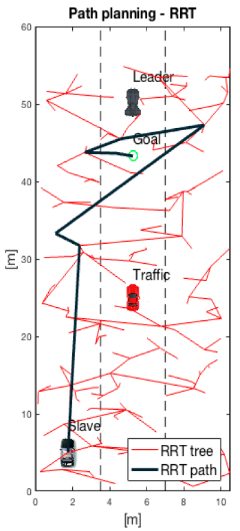
2.1. Path Planning with Rapid-Exploring Random Trees (RRT)

Path planning finds a feasible path for the slave vehicle from its actual position to its target platoon position. In this section, a feasible path is a path that is contained into the road boundaries and that avoids other traffic obstacles including other vehicles.
There are many ways to solve this problem. Path planning has been extensively studied in graph theory and offers therefore plenty different algorithms: Dijkstra algorithm, A* algorithms, etc. [17].
The one chosen in this study is a variant of the Rapid- exploring Random Trees (RRT) [18]. This method fulfils the demands of the path planning task to be efficient (real-time capable) and safe (in face of uncertainty and sensing errors) [19]. The benefits of using a sampling-based method are:
  • There is no need to explicitly characterize the configuration space, but instead probe the space and use collision detection on the go.
  • They are incremental in nature and efficient which offers the potential for real-time implementation while retaining completeness guarantees.
The basic principle of RRT as would be suitable in our context of platoon formation is the following: a tree of trajectories is grown through random sampling [20] of an environment localization map (the God’s eye view) created through data fusion of the sensor data. Samples are added or discarded based on the feasibility.
Although the tree expansion and hence the space exploration is very fast, the simple RRT path has a major drawback: it is highly random.
Figure 4 illustrates an RRT path calculation for the platooning problem. Even though it avoids obstacles and reaches the desired target, it is obvious that this path is not applicable in a real situation.

2.2. Biased RRT Star (RRT*)

RRT* is an evolution of the RRT algorithm [21,22,23]. Instead of connecting each new node to its closest tree node, it connects with the node that reaches it with the least cost (distance).
To accelerate the path finding towards the target position, the sampling of the configuration space is biased: x% of the new samples are taken towards the goal position (x depends on the complexity of the situation, i.e., the number of traffic objects or the shape of the road, but is usually high). This bias enables it to converge faster and create straighter paths. Note that the RRT path will always be biased in the following discussion even if it is not specified.
Figure 5 illustrates biased RRT* path planning for the platooning problem. The RRT* path is less random and quickly reaches the desired position. However, this solution is not optimal. A human driver would rather pick a path on the left of the traffic vehicle.

2.3. Informed RRT* (i-RRT*)

Informed RRT* is again an evolution of the RRT* algorithm. The basic principle is to have an RRT* path search in a restricted configuration space to converge quicker to a close to optimal solution [24]. The limited configuration space is taken as an ellipse whose characteristics are defined by an initial RRT* path.
Figure 6 shows the initial RRT-star path, the ellipse derived from it and the new i-RRT* path found for the platooning problem, showing desirable results.

3. Path Optimization Using Model Predictive Control

Having an initial path planned, and using RRT*, the next important consideration is to optimize it for feasibility. A Model Predictive Control is an optimal control technique that relies on the prediction of future outputs of the considered plant to perform an optimization under constraints of the current time step control action. At each time step, a cost function is minimized over a certain number of future time steps called prediction horizon, calculating and applying to the prediction model a certain number of future control moves called control horizon [25].
The MPC path optimization algorithm is used to generate an optimal vehicle control sequence so that the vehicle follows as accurately as possible the a priori calculated RRT* path, while complying with constraints. These constraints include soft constraints such as acceleration and jerk limits, and physical or hard constraints such as steering angle limits.
The core of the MPC technique relies on a prediction model of the controlled system and for this study we use a kinematic and a dynamic-bicycle model [26,27], which accurately models the vehicle to a desired fidelity, accounting for its dimensions and the geometry.
Once the RRT* algorithm has found an initial path it is used to determine a set of control commands to apply to the slave for it to reach the leader, in an optimal manner using MPC. The considered control variables are the steering angle δ f and the jerk j described by a vector u = ( j δ ) t [28,29].
The RRT* path coordinates can be treated as set points for the slave lateral position, as illustrated in Figure 7. The longitudinal distance between the leader and the slave x * is treated as a cost value to be minimized over the simulation period (prediction horizon). The control and state variables are bounded by the dynamic constraints the slave vehicle must respect. Alongside those constraints the controller aims at not being too demanding on the control variables (jerk and steering angle) since it is a necessity for the vehicle to be gently steered and softly driven.
Next, to solve the prediction model while complying with a certain set of constraints applied to the state and command variables, an optimization problem is solved. For this study, the objective is written as a minimization of the cost function J defined as follows:
a r g m i n u U J = 0 t f q 1 ( y y r ( x * ) ) 2 + q 2 x * 2 + q 3 j 2 + q 4 δ f 2 d t
s u c h     t h a t     { X ˙ ( t ) = A ( t ) X ( t ) + B ( t ) u ( t ) Y ( t ) = C ( t ) X ( t ) + D ( t ) u ( t )  
w i t h   s t a t e : X = ( x       y       x *     v x       v y       a       j       ψ         ψ ˙       δ f       x l e a d e r ) t
a n d   c o n s t r a i n t s { X ( t 0 ) = x 0 t f = 15   s | a | < 3   m / s 2 | j | < 5   m / s 3 v < 130   km / h
Using:
  • y the lateral vehicle coordinate [m].
  • y r the RRT* lateral coordinate [m] (Figure 8).
  • x * the longitudinal distance between leader and slave [m].
  • x l e a d e r the leader longitudinal coordinate [m].
  • ψ ,     ψ ˙ ,     δ f   the heading angle, the yaw rate and the steering angle, respectively [rad].
  • v x ,     v y   the slave lateral and longitudinal speed, respectively [m/s].
  • q i 1 , 2 , 3 , 4 the weights of the cost function [-].
  • t f the prediction horizon (time over which the dynamic model is solved).
The cost function can be interpreted as the cumulative sum over time of four weighted errors using the coefficients ( q i 1 , 2 , 3 , 4 ) . Minimizing J naturally implies minimizing these cumulative errors over the prediction horizon.
The weight coefficients q i 1 , 2 , 3 , 4 are empirically determined by assessing the results of the optimization solver. When setting the MPC controller the value of each q i must be specified. The absolute value of each coefficient taken separately has no meaning but yet their relative values with respect to each other affect the cost function behaviour during minimization. Hence, to minimize an error more than the others, its associated weight in the cost function shall be increased. For instance, a large q 1 / q 2 would yield an optimized path very close to the RRT* reference but would be detrimental to the time to reach the leader. The values listed in Table 1 have been found to yield best results.
The squared error terms are the following:
  • ( y y r ( x * ) ) 2 : deviation between slave lateral position and the RRT* lateral coordinate.
  • x * 2 : distance between the slave and the goal. Minimizing this state variable is the main lever to reach the leader.
  • j 2 : slave jerk. Minimizing the jerk prevents being too demanding on it.
  • δ f 2 : slave steering angle. Same justification as for the jerk.
The dynamic equations of the system X ˙ = A X + B u can either be derived from the dynamic bicycle model or the kinematic one. This implementation of the path planner is possible in any virtual vehicle environment. The choice of the vehicle model will affect the accuracy and robustness of the path planner. Indeed, using the dynamic bicycle model will lead to a better model accuracy but will impede on computational speed. As later discussed in this paper, the higher the path planning frequency, the smaller the discrepancies between actual and predicted slave position.
Next, we consider solving the optimization problem practically. A python package called GEKKO, was used to solve the optimization problem which uses direct transcription method (also call “orthogonal collocation on finite elements”) to minimize the cost function acting on state and control variables. These variables are manipulated to find the optimal solution that minimizes the cost function J. Yet the solver plays on variables so that they respect the system dynamics. In other words, there is at any point in time a valid solution of the system, that is a set of differential equations.

4. Results

4.1. Path Optimization

The previously described optimization problem has been implemented in GEKKO (with a 150 ms discretization of the kinematic bicycle model). Using the kinematic bicycle model as a first try, the results are shown in Figure 8. Applied constraints are listed in Table 2.
Figure 9 shows that for this case the constraints on acceleration, jerk and steering angle were, respectively, 5 m·s−2, 5 m·s−3 and 8°. The blue dashed line represents the jerk for the dynamic bicycle model. Beyond smoothing the jerk of raw RRT* path, the MPC method has provided us with the time profiles of each command variable to be adopted by the slave. The optimization solver finds a kinematically feasible solution while minimizing the deviation between the slave lateral position and RRT* lateral reference coordinate. The optimization has been run for a prediction horizon of 15 s but a 10 s horizon has turned out to be enough to reach the leader. In the early stages of the manoeuvre the acceleration and the jerk control variables hit their limits. Indeed, since the cost function includes the distance to the leader x * , the solver minimizes this quantity over the complete prediction horizon. This results in reaching the leader position as quickly as possible and thus the control variables are asked to operate at their limits as soon as possible.
As briefly previously discussed, the dynamic model choice will impede on path planner accuracy. Figure 9 shows both the optimized path based on a kinematic bicycle model and the one leveraging a dynamic bicycle model. The results slightly differ in terms of command profiles, and indeed the dynamic bicycle turned out to lead to a more aggressive steering angle command.
In the final implementation the path planner runs the RRT* along with an optimization algorithm several times prior to reaching the leader. Throughout the manoeuvre the path planner is called numerous times at a specific frequency to run the calculation as the slave is getting closer to the leader (see Figure 10). This is done so that the path planner could cope with a changing environment. If this frequency is too low, then the time in between each optimization result is longer and the slave travels larger distances. This would lead us to face the risk of having bigger discrepancies between the model-predicted vehicle position and the actual vehicle position when beginning the next path planning calculation.
Therefore, to prevent the path planner from lacking accuracy one should properly set its frequency or should use a more detailed vehicle dynamics model. It is necessary to find the best compromise between a high path planning frequency that would alleviate model inaccuracy (detrimental to computational time) and the use of a more sophisticated vehicle model that would require longer computational time.

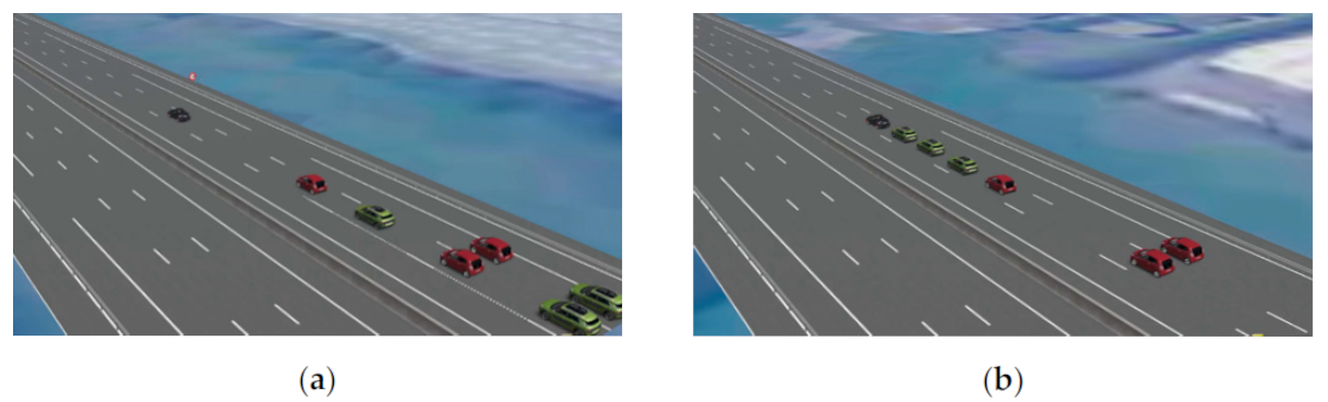
4.2. Simulation Results

After configuring the input and output signals, the platooning and optimization algorithms were implemented in a virtual vehicle environment as depicted in Figure 11, which shows the complete pipeline.
The platoon ordering step accounts for the starting point. At the very beginning of the platooning, the RRT* path planner is run for each platoon candidate. Then, all the candidates are ranked based on their RRT* cost which is the length of the raw RRT* path. The closest candidate will be the first to be steered and driven towards its platoon position. Once it has made its way to its goal, the platoon ordering function is called again to decide the next candidate to join the platoon. This loop is performed until all the candidates have entered the platoon. Changing traffic, moving leader and highway curvature require the frequent repetition the path planner during a candidate attempt to reach the leader. Likewise, the imperfection of the considered dynamic model yields the same path planner execution constraint.
Figure 10 depicts a scenario involving three traffic objects and three platooning candidates. In this case the path planner frequency has been set to f p p = 5   Hz . The left picture is a God’s eye view of the vehicles configuration in a virtual vehicle environment and the right axis shows the path planner results for different time steps. The intensity of the object’s color refers to the time step of the simulation.
At each path planning step, the initial conditions used in the MPC controller are the last vehicle state variables at the last time step. As a result, it is required to feed the MPC controller with the updated candidate and leader states. In this example, the MPC manages to correct the path infeasibilities generated by the RRT* calculation. The slave behaviour is expected to be smoother if we were to use informed i-RRT* instead of conventional RRT*. Indeed, informed RRT* tends to correct non-relevant trajectories yielded by RRT*. Figure 12 shows different frames depicting the platoon being formed. The closest slave gets called first. It finds a trajectory around the traffic in front of it and joins the leader. Then the slave from the back is called second. It avoids the two traffic vehicles in front of it as well as the third vehicle and aims to drive behind the first slave. Finally, the third slave is allowed to join the platoon and finishes the manoeuvre. Each slave had to abide by the constraints given to it as well as keep a safe distance from both the traffic vehicles as well as the other slaves in the platoon. Link to the video: https://drive.google.com/file/d/1weKhGTTy9nHOSGgDcRcBPgzpw-OH8l9X/view?usp=sharing (accessed on 21 April 2021).

5. Discussion

Path planning studies are often proposed pertaining to maintaining a platoon [1,2,3,4]. Cooperative manoeuvring of formed platoons has been studied [9,14] and addition of a new vehicle at highway junctions has been discussed [8,15], but no consideration has been given to platoon formation itself, which would need to be in a dynamic environment. This remains a bottleneck for fully automated co-operative systems. The results from Section 4 indicate that using an initial given scenario (initial positions of vehicles and “leader” on a highway, along with traffic objects), by using a combination of RRT* and MPC, it is feasible to generate optimal paths to be followed for vehicles to join and form a platoon, independent of the initial positions of the vehicles and the traffic objects (non-platooning vehicles). This is possible due to RRT* being computationally cheap along with a kinematic bicycle model of the vehicle for MPC prediction, which permits high frequency update of the path (see Table 3 and Figure 11). RRT* was criticized for its sampling based nature [16] in the context of platooning, but optimizing the initial path from RRT* (via MPC) gives desired results. To the best of our knowledge, no previous work has used this combination in the context of platooning on highways. The average time for a complete path calculation was simulated to be 1.3 s which would be even faster in real-time systems, although this was not studied further in this work. Importantly, we note that calculation of a vehicle’s optimum trajectory to form a platoon while keeping the longitudinal and lateral acceleration to safe limits (below 3 m/s2, and lateral jerk below 5 m/s3) is feasible. This is made possible by the prediction horizon of the MPC of 10 units ahead in time. Furthermore, the trajectory is updated continuously within and thus can deal with varying environments (traffic vehicles changing lanes, for example). Therefore, these results should be taken into account when considering highly automated highway systems.
The validation of this pipeline was done in a virtual vehicle environment, but the implementation is independent of any specific environment and the reader is encouraged to test the merits of the proposed methodology of finding paths for platooning on highways, which represents a constrained environment in terms of the space of possible actions for a given vehicle. Furthermore, the considerations for “slave” vehicles forming a platoon with a “leader” vehicle were required for creating scenarios for the simulation but are not the main focus of the study, which is dynamic path planning for platoon formation and which is independent whether these assumptions hold or not. The outcome (the optimum planned trajectory for platoon formation) can be generated in entirely different settings, unaffected by the above assumptions. To that extent, several shortcomings for the problem of dynamic path planning for platoon formation still need to be treated:
  • Several scenarios are still to be studied (border cases), such as the “leader” being behind “slave” vehicles, or all three lanes being completely blocked by traffic.
  • Although the RRT* algorithm provides us with an obstacle-free trajectory, the MPC controller yields a very close but still different trajectory. There is thus a risk of colliding with obstacles if the path planner frequency is too low. To that extent, the real-time performance in embedded systems is an important aspect to be tested, for example, with hardware in-the-loop modelling. Although the results in simulation show a high frequency path calculation, it must be real-time capable for a given hardware.
  • The path planner implemented here considered no highway driving protocols, such as knowing the legal way to cross lanes, which gives scope for future study. Another important direction is the usage of informed-RRT* which should result in faster converging paths.

6. Conclusions

This work introduces a path planning solution that enables a vehicle to autonomously join a platoon with optimized trajectory robust to uncertain traffic obstacles on highways, bringing us closer to automated highway systems (AHS). To the best of our knowledge, this paper is the first to harness RRT* and MPC to achieve platoon formation on highways in the face of varying initial positions and dynamic obstacles (other vehicles as traffic). Initial results simulated in a virtual vehicle environment show the potential of the method. In particular, the use of RRT* to find the initial path optimized via MPC is both efficient and easy to implement. Our proposed solution has been tested in a virtual vehicle simulation environment with a high fidelity vehicle dynamics model in realistic highway scenarios. This work could also serve as a basis for studies that aim to find optimal paths for platoon formation beyond automated highway systems, in urban environments.

Author Contributions

Conceptualization, O.E.G.-M., S.C. and T.H.; methodology, O.E.G.-M., S.C. and T.H.; software, V.A., M.D.N. and V.A.K.; validation, O.E.G.-M., S.C.,T.H., V.A., M.D.N. and V.A.K.; formal analysis, V.A., M.D.N. and V.A.K.; investigation, O.E.G.-M., S.C. and T.H.; resources, O.E.G.-M.; data curation, O.E.G.-M.; writing—original draft preparation, O.E.G.-M.; writing—review and editing, O.E.G.-M., S.C. and T.H.; visualization, V.A., M.D.N. and V.A.K.; supervision, O.E.G.-M., S.C. and T.H.; project administration, O.E.G.-M. All authors have read and agreed to the published version of the manuscript.

Funding

This research received no external funding.

Conflicts of Interest

The authors declare no conflict of interest.

References

  1. Swaroop, D.; Hedrick, J.K. Constant Spacing Strategies for Platooning in Automated Highway Systems. J. Dyn. Syst. Meas. Control 1999, 121, 462–470. [Google Scholar] [CrossRef]
  2. Peppard, L. String stability of relative-motion PID vehicle control systems. IEEE Trans. Autom. Control 1974, 19, 579–581. [Google Scholar] [CrossRef]
  3. Naus, G.J.L.; Vugts, R.P.A.; Ploeg, J.J.; Van De Molengraft, M.J.G.; Steinbuch, M.M. String-Stable CACC Design and Experimental Validation: A Frequency-Domain Approach. IEEE Trans. Veh. Technol. 2010, 59, 4268–4279. [Google Scholar] [CrossRef]
  4. Xiao, L.; Gao, F. Practical String Stability of Platoon of Adaptive Cruise Control Vehicles. IEEE Trans. Intell. Transp. Syst. 2011, 12, 1184–1194. [Google Scholar] [CrossRef]
  5. Yanakiev, D.; Kanellakopoulos, I. Nonlinear spacing policies for automated heavy-duty vehicles. IEEE Trans. Veh. Technol. 1998, 47, 1365–1377. [Google Scholar] [CrossRef]
  6. Seiler, P.; Pant, A.; Hedrick, K. Disturbance Propagation in Vehicle Strings. IEEE Trans. Autom. Control 2004, 49, 1835–1841. [Google Scholar] [CrossRef]
  7. Shaw, E.; Hedrick, J.K. String Stability Analysis for Heterogeneous Vehicle Strings. In Proceedings of the 2007 American Control Conference, New York, NY, USA, 9–13 July 2007; pp. 3118–3125. [Google Scholar]
  8. Dao, T.S.; Huissoon, J.P.; Clark, C.M. A strategy for optimization of cooperative platoon formation. Int. J. Veh. Inf. Commun. Syst. 2013, 3, 28–43. [Google Scholar]
  9. Hobert, L.H.X. A Study on Platoon Formations and Reliable Communication in Vehicle Platoons. Master’s Thesis, University of Twente, Enschede, The Netherlands, 2012. [Google Scholar]
  10. Sheikholeslam, S.; Desoer, C.A. Longitudinal Control of a Platoon of Vehicles. In Proceedings of the 1990 American Control Conference, San Diego, CA, USA, 23–25 May 1990; pp. 291–296. [Google Scholar]
  11. Tuchner, A.; Haddad, J. Vehicle platoon formation using interpolating control: A laboratory experimental analysis. Transp. Res. Part C Emerg. Technol. 2017, 84, 21–47. [Google Scholar] [CrossRef]
  12. Rosenzweig, J.; Bartl, M. A Review and Analysis of Literature on Autonomous Driving. 2015. Available online: https://michaelbartl.com/wp-content/uploads/Lit-Review-AD_MoI.pdf (accessed on 21 April 2021).
  13. Young, B.J.; Beard, R.W.; Kelsey, J.M. A Control Scheme for Improving Multi-Vehicle Formation Maneuvers. In Proceedings of the American Control Conference. (Cat. No.01CH37148), Arlington, VA, USA, 25–27 June 2001; Volume 2, pp. 704–709. [Google Scholar]
  14. Lam, S.; Katupitiya, J. Cooperative Autonomous Platoon Maneuvers on Highways. In Proceedings of the 2013 IEEE/ASME International Conference on Advanced Intelligent Mechatronics, Wollongong, NSW, Australia, 9–12 July 2013; pp. 1152–1157. [Google Scholar] [CrossRef]
  15. Lu, X.-Y.; Tan, H.-S.; Shladover, S.E.; Hedrick, J.K. Automated Vehicle Merging Maneuver Implementation for AHS. Veh. Syst. Dyn. 2004, 41, 85–107. [Google Scholar] [CrossRef]
  16. Claussmann, L.; Revilloud, M.; Gruyer, D.; Glaser, S. A Review of Motion Planning for Highway Autonomous Driving. IEEE Trans. Intell. Transp. Syst. 2020, 21, 1826–1848. [Google Scholar] [CrossRef] [Green Version]
  17. LaValle, S.M. Motion Planning: The Essentials. IEEE Robot. Autom. Mag. 2011, 18, 79–89. [Google Scholar] [CrossRef]
  18. Lavalle, S.M. Rapidly-Exploring Random Trees: A New Tool for Path Planning, from the Annual Research Report. 1998. Available online: http://citeseerx.ist.psu.edu/viewdoc/citations;jsessionid=A1AB62F78BC767D0F82777B22AA4B79C?doi=10.1.1.35.1853 (accessed on 21 April 2021).
  19. Kuwata, Y.; Karaman, S.; Teo, J.; Frazzoli, E.; How, J.P.; Fiore, G.A. Real-Time Motion Planning With Applications to Autonomous Urban Driving. IEEE Trans. Control Syst. Technol. 2009, 17, 1105–1118. [Google Scholar] [CrossRef]
  20. Cheng, P.; LaValle, S.M. Reducing Metric Sensitivity in Randomized Trajectory Design. In Proceedings of the 2001 IEEE/RSJ International Conference on Intelligent Robots and Systems. Expanding the Societal Role of Robotics in the Next Millennium (Cat. No.01CH37180) 1, Maui, HI, USA, 29 October–3 November 2001; Volume 1, pp. 43–48. Available online: https://pdfs.semanticscholar.org/15e7/f233088f52dffadc0b07b5ff90ad69a71323.pdf (accessed on 21 April 2021).
  21. Karaman, S.; Frazzoli, E. Sampling-based algorithms for optimal motion planning. Int. J. Robot. Res. 2011, 30, 846–894. [Google Scholar] [CrossRef]
  22. Islam, F.; Nasir, J.; Malik, U.; Ayaz, Y.; Hasan, O. RRT-Smart: Rapid Convergence Implementation of RRT towards Optimal Solution. In Proceedings of the IEEE International Conference on Mechatronics and Automation, Chengdu, China, 5–8 August 2012; pp. 1651–1656. [Google Scholar]
  23. Nasir, J.; Islam, F.; Ayaz, Y. Adaptive Rapidly-Exploring-Random-Tree-Star (RRT*)-Smart: Algorithm Characteristics and Behavior Analysis in Complex Environments. APIJTM 2013, 2, 39–51. [Google Scholar] [CrossRef]
  24. Gammell, J.D.; Srinivasa, S.S.; Barfoot, T.D. Informed RRT*: Optimal Sampling-Based Path Planning Focused via Direct Sampling of An Admissible Ellipsoidal Heuristic. In Proceedings of the International Conference on Intelligent Robots and Systems, Chicago, IL, USA, 14–18 September 2014; pp. 2997–3004. [Google Scholar] [CrossRef] [Green Version]
  25. Melda Ulusoy, M. Understanding Model Predictive Control, Part 3: MPC Design Parameters Video—MATLAB & Simulink. 2018. Available online: https://fr.mathworks.com/videos/understanding-model-predictive-control-part-3-mpc-design-parameters-530607670393.html (accessed on 21 April 2021).
  26. Ren, H.; Shim, T.; Ryu, J.; Chen, S. Development of Effective Bicycle Model for Wide Ranges of Vehicle Operations; SAE Technical Paper Series; SAE World Congress & Exhibition: Warrendale, PA, USA, 2014. [Google Scholar] [CrossRef]
  27. Kong, J.; Pfeiffer, M.; Schildbach, G.; Borrelli, F. Kinematic and Dynamic Vehicle Models for Autonomous Driving Control Design. In Proceedings of the IEEE Intelligent Vehicles Symposium (IV), Seoul, Korea, 28 June–1 July 2015; pp. 1094–1099. Available online: http://me.berkeley.edu/~frborrel/pdfpub/iv_kinematicmpc_jason.pdf (accessed on 21 April 2021). [CrossRef]
  28. Polack, P.; Altché, F.; d’Andréa-Novel, B.; de La Fortelle, A. Conference: 2017 IEEE Intelligent Vehicles. Available online: https://www.researchgate.net/publication/318810853_The_kinematic_bicycle_model_A_consistent_model_for_planning_feasible_trajectories_for_autonomous_vehicles (accessed on 21 April 2021).
  29. Schmitt, C.J.; Basset, M.; Gissger, G.L. European Control Conference, ECC 1999—Conference Proceedings. 2015. Available online: https://www.researchgate.net/publication/267228739_Identification_of_physical_parameters_of_a_passenger_car (accessed on 21 April 2021).
Figure 1. Platoon formation illustration.
Sustainability 13 04668 g001
Figure 2. Vehicle system architecture for autonomous platooning.
Sustainability 13 04668 g002
Figure 3. General operation flow of platoon formation.
Sustainability 13 04668 g003
Figure 4. Path planning with RRT.
Sustainability 13 04668 g004
Figure 5. Path planning with RRT*.
Sustainability 13 04668 g005
Figure 6. Path planning with i-RRT*.
Sustainability 13 04668 g006
Figure 7. Raw RRT* path and leader-ego x * distance to minimize.
Sustainability 13 04668 g007
Figure 8. Results of the optimization solver using a kinematic bicycle model.
Sustainability 13 04668 g008
Figure 9. Comparison of the optimization solver results using kinematic and dynamic bicycle models.
Sustainability 13 04668 g009
Figure 10. Configuration example with a leader, three slaves and three traffic vehicles.
Sustainability 13 04668 g010
Figure 11. Path planner implementation pipeline.
Sustainability 13 04668 g011
Figure 12. Beginning (a) and end frames (b) of the vehicles forming the platoon.
Sustainability 13 04668 g012
Table 1. Values of the cost function weights.
Weight q 1 q 2 q 3 q 4
Value1505501
Table 2. Constraints on state and control variables.
State Variablevxa     ψ ˙ j δ f
Minimum0 m/s−5 m/s2−10°/s−5 m/s3−10°
Maximum30 m/s5 m/s210°/s5 m/s310°
Table 3. Computational time for both models.
Bicycle ModelComputational Time
Kinematic1.3 s
Dynamic1.6 s
Publisher’s Note: MDPI stays neutral with regard to jurisdictional claims in published maps and institutional affiliations.

