The Ideal Debt Ratio of an Agricultural Enterprise

Abstract

The objective of the contribution is to propose a new methodology for determining the optimal credit absorption capacity of an enterprise while maintaining the positive function of financial leverage, i.e., the maximum possible loan that would continuously bring benefit to the enterprise. The proposed methodology determines the credit absorption capacity of an enterprise according to EVA Equity and EVA Entity. Based on a theoretical analysis of both indicators, the possibility of applying the proposed methodology for this purpose was proved. To verify the theoretical assumptions, the optimal credit absorption capacity of enterprises operating in the agricultural sector of the CR was determined. The data used for the purposes of the contribution were obtained from the Albertina database for the years 2012–2018. The credit absorption capacity of the monitored enterprises ranged from CZK 6.88 million to CZK 9.6 million. The article also determines the optimal ratio of equity to debt capital.

1. Introduction

A key objective of an enterprise as it matures is growth in value for shareholders. Business owners and investors consider it important to use effective tools for determining the value for a specific period of time. Economic Value Added (EVA) is currently the most effective economic tool for the profit rate (performance) assessment. Since the EVA indicator also considers alternative costs of equity, EVA is one of the most popular tools to determine an enterprise’s profit rate. This indicator might also be regarded as an indicator of the actual profit rate for owners, investors, shareholders, partners, and other stakeholders. A positive EVA indicator shows the appreciation rate of a specific investment to the value of other investments at the same level of risk. A potential negative EVA indicator would demonstrate that the investment in such an enterprise constitutes a higher risk for the creditor compared to the same level of investment made in a different enterprise. With respect to the effectiveness of using the EVA indicator in the Czech environment, this method is widely discussed. To achieve a positive EVA indicator value, it is necessary to follow the relevant methodology. The information about the value of this indicator cannot be commonly derived from the financial statements of enterprises created in accordance with the legislation of the CR. The EVA indicator shows the closest relationship between the values of shares, which may be demonstrated by statistical calculations [1]. This indicator enables the use of information and data obtained from financial statements, including the data based on which the financial statements were compiled. The calculation of the EVA indicator includes calculations of the risks for business owners and potential investors since the input variables for the calculation of this indicator consist of some components reflecting this risk. These are thereby calculated outside the resulting equation for calculating the EVA indicator. Finally, it enables the assessment and valuation of an enterprise.

As far as investors are concerned, the best enterprises to invest in are those with the highest possible EVA indicator value. All entrepreneurs or investors should be aware of the appreciation rate of their specific investment. The essential prerequisite for generating the value added of an enterprise is the level of profits and the highest possible efficiency of its capital. As for business owners, the EVA indicator represents a useful tool to decide how and to what extent to invest capital in order to generate further profits. This decision can also involve investments in various projects.

The total capital of an enterprise consists of different ratios of equity and debt capital. At the same time, every enterprise should strive to achieve the optimal ratio of both components of capital. However, this article will only consider the capital employed (CE).

The optimal ratio of debt capital is achieved when the business risk is reduced to the minimum and the contribution of the debt capital is the highest. The subject of the analysis is therefore to determine the optimal share of debt capital in an enterprise using the EVA indicator. The proposed methodology is demonstrated on a sample of enterprises operating in the agricultural sector in the CR.

The objective of this article is to analyze the credit absorption capacity in the agricultural sector in the period 2012–2018. For this purpose, two hypotheses were formulated:

• It is possible to determine the credit absorption capacity of the agricultural sector on the basis of the difference in values of EVA Entity and EVA Equity.
• Financial leverage has a positive effect on the agricultural sector.

In the case of agricultural enterprises, EVA indicators can determine the effectiveness of the capital investment in boosting their crop and livestock production. In the case of increased investment, increased costs due to the possible construction of new premises for storing boosted crop production or stabling additional heads of livestock need to be taken into consideration as well. What also must not be omitted are the costs related to the operation of such facilities, costs of mechanization, and the incremental costs of fuels and wages.

The structure of this article is as follows: the literature review related to the topic is followed by an explanation of the theoretical background that forms the basis of this article. The methods applied and all the necessary input data are subsequently described. The presentation of the achieved results is followed by a discussion and a summary of the results.

2. Literature Review

Most owners of small and large enterprises in the CR are insufficiently informed about the possibility of debt financing their companies. This can be caused by a lack of managerial skills or business know-how; more experienced owners are also better aware of the risks associated with loans [2]. Requirements for company financing may differ throughout a company’s life cycle. An enterprise decides upon debt financing according to types of projects in order to increase its profit rate. However, enterprises decide upon debt financing in the event that unexpectedly high extraordinary (and operating) costs will be incurred [3]. Moritz et al. [4] identified different methods of financing small and medium-sized enterprises in Europe. In addition to debt financing, they also identified five other methods of financing enterprises, including combined financing, state contributory financing, flexible debt financing, business financing, and internal financing. Florou and Kosi [5] examined the influence of the mandatory adoption of International Financial Reporting Standards (IFRS) on the debt financing of enterprises in the market. They concluded that by adopting IFRS, and in the event of debt financing, enterprises resorted to issuing bonds rather than taking loans from commercial banking institutions. Gonzáles [6] focused on the maturity of company debt in times of financial crisis. The cash-flow solvency of enterprises that were more dependent on debt financing than enterprises that used a larger part of equity for financing sharply declined within this period.

Altunbas et al. [7] state that if debt financing of an enterprise is required, individual enterprises use different ways to obtain these financial resources. The choice depends on the overall size of the enterprise. Large enterprises, which tend to borrow larger amounts of financial resources, are inclined to meet their financial needs through syndicated loans. On the other hand, small enterprises tend to sell corporate bonds to satisfy their financial requirements. According to Yazdanfar and Öhman [8], medium-sized enterprises should focus on finding the optimal level of debt financing as current debt policy significantly affects future corporate performance. On the other hand, Chua et al. [9] argue that small enterprises tend to rely on family members to cover debt financing since these enterprises fail to meet the requirements of banking institutions for granting loans. Klieštík and Cug [10] analyzed four methods of describing credit risks. From this point of view, credit absorption capacity can be considered as the level of credit risk for creditors.

Zheng et al. [11] conducted research focused on finding a relationship between the national culture of individual states and the solvency of enterprises/the ability of enterprises to meet their financial obligations. They point out that enterprises in countries with a high degree of financial insecurity, collectivism, and masculinity tend to take short-term loans. Degryse et al. [12] analyzed differences in the solvency of their credit obligations with respect to corporate ambitions. They found that small and medium-sized enterprises try to cover their debts using generated financial surpluses. However, in the event that these enterprises have ambitions to grow, only short-term loans are paid from this resource, which means a growth in the volume of long-term loans. Gilson [13] argues that transaction costs are also one of the factors that may discourage enterprises from reducing their debts. According to Almazan et al. [14], the volume of long-term loans is affected by the locality of specific enterprises. In developing or developed cities with many opportunities to set up a business, enterprises make efforts to use these opportunities by taking greater long-term loans. Lin et al. [15] analyzed the ownership structure of enterprises and costs related to their debt financing. The results showed that business owners are severely threatened if shareholders are the majority owners of the enterprise; i.e., the owner of the enterprise loses control over corporate cash flows so that shareholders can easily use corporate assets.

An excessively high volume of debt capital results in a negative financial leverage effect. Harford et al. [16] analyzed the capital structure of enterprises that strive to achieve the maximum leverage effect. In the event that the level of the leverage effect is above the target level, these enterprises are likely to finance further business development from equity. Denis and McKeon [17] found that enterprises intentionally maximized the leverage effect to cover their operating costs. However, the reduction of corporate debt is slow. Enterprises resort to reducing the leverage effect only in the event that the enterprise generates a financial surplus. On the other hand, enterprises facing financial deficits tend to cover this deficiency of financial resources by further magnifying the leverage effect. Ghosh and Moon [18] dealt with the issue of the relationship between corporate debt financing and the positive impact on corporate profit quality. They argue that in the event of debt financing, enterprises focus on covering the costs of their debts rather than on profit quality, as penalties from breaching loan agreements significantly exceed the costs of the loan itself.

To optimize the volume of debts, it is important to analyze the correlation between financial leverage and enterprise performance. This was analyzed by Abu-Abbas et al. [19], who state that financial leverage shows a negative correlation with ROA (return on assets) and EVA indicators of enterprise performance. Extremely negative correlations between these indicators and financial leverage were observed in enterprises that followed the product differentiation strategy. Liang [20] argues that enterprises are able to absorb debt capital more effectively if investments in the enterprise are made and, also, in the event that these enterprises adopt new technologies and manufacturing processes from a specific creditor. In such a case, however, there is no increase in the number of foreign customers. According to Tsuruta [21], highly indebted small enterprises are not able to obtain sufficient loans to optimize the leverage effect and may therefore lose potential profits. On the other hand, efficient small enterprises can use the loans obtained to further improve their performance. This statement was verified on a sample of small enterprises operating in Japan. Furthermore, small enterprises with sufficient collateral assets and a high degree of positive financial leverage show better performance [22]. Based on the results of an analysis of the business sector, Mallinguh et al. [23] found that the performance of an enterprise is influenced by its age, the degree of foreign ownership, and the function of financial leverage.

The effect of the credit absorption capacity can be measured using the indicators of Economic Value Added (EVA). The EVA indicator is widely considered to be a key indicator of business performance. The adoption of this indicator occurred as industry started to move from the production world of the past to the production world of the future, which is highly focused on value. The EVA indicator is a specific type of economic profit that indicates that in order to achieve tangible profits, an enterprise needs to generate sufficient profit not only to cover its operating costs, but also to cover capital costs [24]. Girotra and Yadav [25] declare that the intensifying competition on the market requires new indicators to inform business owners and shareholders about the performance of the enterprise in question. This is achieved through EVA indicators, which are a new set of indicators available to managers and shareholders. Nevertheless, this is not a tool for accumulating business wealth for shareholders and investors; it is rather a tool for making shareholders and investors behave as business owners and strive for improved performance. The authors recommend shareholders and investors extensively explore the whole market and then make a decision on possible investments, i.e., they should not only consider EVA indicators because the ever-changing market environment may not correspond to the actual state of the enterprise.

In the People’s Republic of China, the EVA indicator is used as an indicator of business performance by the local government sector, thereby replacing Return On Equity indicators (ROE), as well as the private sector. Henceforth, EVA indicators became the background for all government decisions regarding private enterprises, which later turned out to be unfair to all private enterprises. Managers therefore started to use both indicators (ROE and EVA) to assess enterprises, using them to modify their preferences so that unfair conduct is avoided [26]. Within this context, Mareček and Rowland [27] used ROE and EVA correlations to determine whether there is a direct relationship between these indicators. The results showed that EVA Equity does not depend on ROE.

Torella and Brusco [28] analyzed the development of enterprises before and after the introduction of the EVA indicator, focusing primarily on the effect of the EVA indicator on the profit rate, investments, and cash-flows. Of major interest is that, on a short-term basis, the EVA indicator did not have any significant impact on them. In the event of poor business performance, the indicator improves only long after the introduction of the EVA indicator. Riceman et al. [29] therefore analyzed whether business managers that regularly use the EVA indicator are able to achieve better business performance than managers who do not apply this indicator. The results of the analysis showed that managers who used the EVA indicator were more successful in achieving better business performance. Analogue research was conducted by DeFeo et al. [30], who focused on assessing business performance using binary logistic regression. In spite of the widespread assumption about the EVA indicator presented by the Stern Steward Company, enterprises that use this indicator tend to be weaker in terms of administration and management than enterprises that do not rely on this indicator. Machová and Vrbka [31] applied the EVA indicator to identify value generators in the agricultural sector. They used neural networks to measure the impact of individual variables on the EVA indicator value (as a relevant enterprise value indicator).

Based on these assumptions, the identification of EVA indicator deficiencies in terms of discovering their causes and proposing measures to remedy them has been the focus of meticulous attention. Biddle et al. [1] formulated a hypothesis on the best indicator of business performance (EVA) using statistical tests. However, the hypothesis was rejected for several possible reasons: (1) the research was based on up-to-date data, not on future cash-flows; (2) the methodology of the valuation of the enterprise adopted from the Stern Steward database was unreliable for the current market and was modified for current clients of this enterprise; (3) the data for calculating the EVA indicator could not be used and the monitored market only had data available that was less than 3 months old; and (4) other unspecified reasons. On the other hand, Forker and Powell [32] analyzed the EVA indicator and its deficiencies in comparison with other methods of business valuation in American and British enterprises. The input data reflected that, compared to generally accepted accounting principles (GAAP), the EVA indicator shows smaller deficiencies in the valuation of enterprises. The EVA indicator also has the smallest prediction deviation from the actual future state of an enterprise. Warr [33] also points to the deficiency of a long-term prediction of business performance using the EVA indicator, whose size is directly proportional to the length of the predicted period as a result of year-on-year inflation.

In terms of the identified EVA indicator deficiencies, this indicator was analyzed in detail in scientific studies comparing the EVA indicator results with those of other economic indicators. Alimeid et al. [34] argue that using EVA enables the improvement of business performance since the decisions made within a specific enterprise will be based on the information on costs related to capital formation. Gupta and Sikarwar [35] mention that the EVA indicator contains added information for shareholders compared to other economic indicators. Bin Ismail [36] focused on the increase or decrease in value of an enterprise in relation to the EVA indicator value. The author concluded that with positive EVA indicator values, an enterprise’s value grows faster than it decreases if the EVA indicator shows negative values.

The authors compared the EVA indicator with share prices, which is also indicative of an enterprise’s value. It was found that the correlation between the EVA indicator and income from shares is a sufficiently reliable tool to determine the value of an enterprise. By combining share prices with the EVA indicator, it is possible to prevent the disturbance resulting from the use of other performance indicators. For that reason, Elali [37] compared the effect of the EVA Equity indicator with Tobin’s Coefficient Q and total shareholder return (TSR). The author also analyzed the relationship between market value added indicators (MVA) and EVA. It was concluded that MVA and EVA bear a closer relationship than that between Tobin’s Q, TSR, and EVA. It was also found that the EVA indicator is only significant in univariate regressions, compared to the combination of Tobin’s Q with TSR in multivariate regressions. This conclusion is supported by the finding that the EVA indicator provides the best information on value for shareholders. According to Harumová [38], the EVA indicator may determine the value of claims a company has in its position as a creditor to other companies. Kryzanowski and Mohsni [39] examined the return on investments in the purchasing price and the difference between the return on investment value and the EVA indicator on a sample of Canadian enterprises in the years 1961–2003. Estimates of capital costs ranged from 9.09% to 12.39%. Returns in the health and IT sectors showed a negative EVA indicator value after measures for compensating costs or risk were imposed. Carlucci et al. [40] analyzed the relationship between value added intellectual connection (VAIC) and EVA using correlation analysis. The tests proved that these indicators do not bear any significant relationship because the EVA indicator is based on financial theory, whereas the VAIC indicator focuses on the effectiveness of intellectual capital. The authors also argue that although business managers see EVA as an invaluable indicator, in order to correctly determine business performance, they recommend using multi-criterion methods. Mittal et al. [41] examined the relationship between EVA indicator value, MVA, and the presence of a code of ethics in enterprises. They did not find any relevant proof that establishing and following a code of ethics in enterprises has any influence on the EVA and MVA indicators.

In a period of economic crisis, markets experience a very specific and non-favorable state. Pavelková et al. [42] analyzed the way EVA value behaves on an example of enterprises in the automotive sector in the period before and after an economic crisis. It was found that value added was the indicator with the deepest negative impact on the value of the EVA indicator. It was also determined that enterprises in the automotive sector showed very similar EVA indicator values in the period of economic crisis.

Vochozka and Machová [43] determined the degree of dependency of the EVA Equity indicator on individual entries of the financial statement of a specific enterprise in the construction industry. The economic growth within the common accounting period, equity, bank loans and financial aids, claims from business transactions, and current assets were identified as the most important entries in financial statements.

Stehel and Vochozka [44] applied EVA Entity and EVA Equity to transport companies in the Czech Republic and compared both indicators using statistical tests. The analyzed enterprises were divided according to several criteria (size, number of employees, and management methods). The results showed that the highest value is generated by those enterprises subject to the national government.

Bolton and Scharfstein [45] examined the optimal number of creditors from whom an enterprise should borrow financial resources to run its business and avoid debts that would be impossible to repay. To determine the optimal number of creditors, there are always a large number of important factors to be considered, such as the nature of the enterprise, quality of the applied technology, and business rating.

Table 1. Overview of the main findings in publications on similar topics.

Author	Year	Main Findings
[1]	1997	The EVA indicator shows the closest relationship to the value of shares.
[4]	2016	Identification of various types of financing for small and medium-sized enterprises in Europe.
[5]	2015	Following the adoption of IFRS, enterprises ensure their debt financing by means of issuing bonds.
[10]	2015	Credit absorption capacity can be seen as the level of credit risk for creditors.
[14]	2010	The sum of long-term loans depends on the location of the seat of the business.
[15]	2011	Shareholders as majority owners pose a threat to business owners.
[16]	2009	A high leverage effect indicates the use of equity for the development of a business.
[18]	2010	Indebted businesses focus on debt repayments instead of the quality of earnings.
[19]	2019	Financial leverage is negatively related to the performance indicators ROA and EVA.
[21]	2015	Highly indebted small enterprises are not able to obtain sufficient loans to optimize the leverage effect and may therefore miss out on potential profits.
[26]	2018	EVA is a fair indicator for evaluating various types of businesses.
[27]	2017	EVA Equity is not dependent on the value of ROE.
[29]	2002	The use of EVA enables a business to achieve better performance.
[32]	2011	EVA shows a lower error rate in determining the value of a business than GAAP.
[33]	2005	Long-term predictions of business performance using EVA show a certain error rate.
[34]	2016	The use of EVA enables improved business performance.
[35]	2016	Compared to other economic ratios, EVA provides higher information value, especially for shareholders.
[36]	2011	With positive EVA values, the growth of business value is faster than the decrease in value associated with negative EVA values.
[37]	2006	The relationship between MVA and EVA is closer than the relationship between Tobin´s Q, TSR, and EVA.
[38]	2003	EVA can be used to determine the value of a company´s receivables.
[41]	2008	Adherence to a corporate code of ethics has an effect on EVA and MVA.

Source: The Authors.

presents an overview of the findings obtained through the analysis of publications on similar topics related to this paper.

3. Theoretical Background

In this section, a theoretical analysis of the EVA Equity and EVA Entity indicators is carried out. The tests are conducted using mathematical calculations and other in-depth analyses of previously presented methods for calculating both EVA indicators. This section can be considered an explanation of the processes, the results of which represent the major contribution this article makes to this field. The calculation of the EVA Equity indicator is carried out using Equation (1) [46].

$$EV{A}_{Equity}=\left(ROE-r_e\right)\ast E$$

(1)

where ROE is return on equity; r_e is costs of equity; and E is equity.

Return on equity is calculated using Equation (2) [46].

$$ROE=\frac{EAT}{E}$$

(2)

where EAT is earnings after taxation; and E is equity.

The Capital Asset Pricing Model (CAPM) is one of the applicable methods for calculating costs of equity. Under this method, the costs of equity are calculated according to Equation (3).

$$r_e=E\left(R_i\right)=r_f+\beta \ast \left(E\left(r_m\right)-r_f\right)$$

(3)

where r_f is risk-free rate of return; β is a factor index of a quantity measuring a systematic risk of a specific asset; and E(r_m) − r_f is a risk premium.

The EVA Entity indicator is calculated according to Equation (4) [47].

$$EV{A}_{Entity}=EBIT\ast \left(1-t\right)-WACC\ast IC$$

(4)

where EBIT is earnings before interest and taxes; t is income tax rate for legal entities; WACC is weighted average capital costs; and IC is invested capital including equity and interest-bearing debt.

To calculate the EVA Entity indicator, it is necessary to determine earnings before interest and taxes (EBIT). EBIT is determined in two steps using Equations (5) and (6). First, earnings before taxes (EBT) must be calculated, based on which the EBIT value is determined after interest costs have been added.

$$EBT=EAT+income tax on common and extraordinary activities$$

(5)

$$EBIT=EBT+interest costs$$

(6)

where EAT is earnings after taxes; and EBT is earnings before taxes.

As the income tax of legal entities was consistent throughout the monitored years, this value equals a rate of 19%. Furthermore, a calculation of weighted average capital costs (WACC) needs to be carried out. WACC is calculated as follows (see Equation (7)).

$$WACC=r_d\ast \left(1-t\right)\ast \frac{D}{C}+r_e\ast \frac{E}{C}$$

(7)

where r_d is cost of deb capital; D is debt interest-bearing capital; C is total capital; r_e is cost of equity; and E is equity.

Debt capital costs (r_d) are calculated according to Equation (8).

$$r_d=\frac{interest costs}{debt capital}$$

(8)

An in-depth theoretical analysis of the EVA Equity and EVA Entity indicators demonstrates a strong mutual relationship between both indicators. If equity is only used to run a business, then only those variables that express the equity of the enterprise, together with the associated costs, can be used as the input data to calculate the EVA Entity indicator. In such a case, the relationship described in Equation (9) is applied.

$$C=E$$

(9)

In the event that the hypothesis is applicable, it can be concluded that the amount of debts (D) equals zero. This implies that the result of the left side of Equation (7) is zero. As a result, the right side of this equation is also greatly simplified. The mathematical expression of the resulting relationship applicable in this case is described in Equation (10).

$$\begin{gathered} WACC=r_d\ast \left(1-t\right)\ast \frac{D}{C}+r_e\ast \frac{E}{C}=r_d\ast \left(1-t\right)\ast \frac{0}{E}+r_e\ast \frac{E}{E}=0+r_e\ast 1 \\ WACC=r_e \end{gathered}$$

(10)

At the same time, it shall be taken into account that there is no reason to consider interest costs (I) when calculating the EVA Entity indicator in this phase, since debt (D) will again equal zero. The mathematical expression of this hypothesis is described in Equation (11).

$$\begin{gathered} I=r_d\ast D=r_d\ast 0=0 \\ I=0\to EBIT=EBT \end{gathered}$$

(11)

After reasonable mathematical modifications, the equation for calculating EVA Entity is as follows (see Equation (12)):

$$EV{A}_{Entity}=EBT\ast \left(1-t\right)-r_e\ast E$$

(12)

It is evident that Equation (12) contains an equation for calculating EAT. After necessary modification, the resulting form of the modified EVA Entity calculation was achieved (see Equation (13)):

$$EV{A}_{Entity}=EAT-r_e\ast E$$

(13)

By multiplying EVA Equity, which is commonly written according to Equation (1), the relationship described in Equation (14) is obtained:

$$EV{A}_{Equity}=ROE\ast E-r_e\ast E$$

(14)

Further decomposition of return on equity (ROE) provides a more detailed form of Equation (14). The resulting decomposition is expressed by Equation (15) as follows:

$$EV{A}_{Equity}=\frac{EAT}{E}\ast E-r_e\ast E$$

(15)

By reducing the variables in this decomposed equation (Equation (15)), the relationship illustrated in Equation (16) is obtained:

$$EV{A}_{Equity}=EAT-r_e\ast E$$

(16)

This means that if the capital of an enterprise was only composed of equity and its costs, the theoretical calculations of both EVA indicators would be identical.

In other words, the ratio between the EVA Entity and EVA Equity indicators indicates the credit absorption capacity of an enterprise. This relationship is expressed in Equation (17).

$$\frac{EV{A}_{Entity}}{EV{A}_{Equity}}=I-r_d\ast \left(1-t\right)\ast D$$

(17)

where I is the absolute value of the interest rate.

The theoretical analysis of both EVA indicators demonstrates that the difference between EVA Entity and EVA Equity provides information on the volume of debt capital together with its costs expressed in absolute values. Based upon these theoretical concepts, under which the mathematical decomposition of both EVA indicators was carried out, it can be concluded that the difference between EVA Entity and EVA Equity enable the credit absorption capacity of an enterprise to be determined. The results of the theoretical analysis therefore confirm the first formulated hypothesis.

4. Data and Methods

The input data was obtained from the Albertina Database [48]. The data contains information about enterprises with a focus on agriculture. According to the classification of economic activities (CZ NACE), this concerns section ‘A’ (agriculture, forestry, fishing, etc.). Data from subclass 01 (Plant and animal production, game-keeping, and associated activities), 02 (Forestry and lumbering), and 03 (Fishing and aquaculture) for the period 2012–2018 were used.

Firstly, the data were divided according to year. The data representing economic indicators of enterprises for periods older than one year were subsequently removed. In addition, enterprises whose input data values were unreasonably negative or, on the contrary, extremely high, incomplete, etc., were also removed. To make the calculation even more precise, those enterprises whose ROE was not in the interval <-100%; 100%> were excluded, as were those enterprises with a debt ratio outside the interval <0%; 200%> and whose economic indicators showed unreasonably negative values. The data includes the value of bank loans and financial aids, total assets, interest costs, inventories, and debt capital. The data were also cleansed of information not relevant to the calculation of the EVA Equity and EVA Entity indicators, as well as the data necessary for calculating the individual steps, i.e., only reliable data were retained. The data used therefore included financial statements, economic results for the accounting period, equity, income tax on common and extraordinary activities, interest costs, and debt capital. Moreover, the removed data included enterprises with missing important data, the presence of which would significantly distort the calculation of the EVA Equity and EVA Entity indicators.

The data subsequently needed to be complemented with further publicly available information. For example, risk-free earnings, more specifically the earnings yield on 10-year government bonds, which was taken from the information portal of the Czech National Bank [49]. Additional data were then added along with a risk premium for the monitored years. These data, including the value of the β unlevered indicator, came from online websites [50].

The yields on 10-year government bonds for the years 2012–2018, risk premium for the monitored years, and the value of the β unlevered indicator are presented in

Table 2. For the years 2012–2018: yields on 10-year government bonds (according to the Maastricht criteria in %), risk premium (in %), and β unlevered indicator (in %).

Year	Risk-Free Rate (%)	Risk Premium (%)	β unlevered (%)
2012	1.92	1.28	0.59
2013	2.20	1.28	0.69
2014	0.67	1.05	0.57
2015	0.49	1.05	0.37
2016	0.53	1.11	0.36
2017	1.50	1.00	0.33
2018	2.01	0.81	0.42

Sources: [49,50]; the Authors.

.

Subsequently, it was necessary to calculate the EVA Equity indicator (Equations (1)–(3)) and EVA Entity indicator (Equations (4)–(8)). These equations are specified in the section describing the theoretical background of this article.

After EVA Equity and EVA Entity were calculated, all the input data necessary to calculate these indicators were subjected to arithmetic means for each monitored year. Although the source dataset did not contain the same number of enterprises for the analysis for all the monitored years, it can be considered a fairly complex dataset capable of generating average values for the individual years. By undertaking this step, a theoretical average enterprise in the agricultural sector in a specific year was created. The achieved results were then presented in the form of a graph. Using the differences in the values of EVA Entity and EVA Equity, the debt absorption capacity was determined for each individual monitored year.

The focus of this article subsequently shifts to determining the answers to the formulated hypotheses. The first hypothesis was already confirmed on the basis of the theoretical background. To obtain the answer to the second hypothesis, a set of diagrams according to individual years was compiled; these diagrams represent the relationships between ROE and the debt ratio of enterprises in the agricultural sector. These diagrams include a trend curve. If the curve shows an upward tendency, this indicates a positive financial leverage effect for a specific debt ratio. According to the effectiveness of the financial leverage for the debt ratio, debt ratio intervals for enterprises in the agricultural sector were determined. These debt ratio intervals with a positive effect on financial leverage were subsequently compared to the debt ratio of the average enterprise for the individually monitored years. The results and follow-up recommendations are discussed in the next section of this article.

5. Results

After removing and complementing the input dataset, the EVA Equity and EVA Entity indicators were calculated. Upon taking all the necessary steps for the calculation described in the theoretical background, the achieved results were as follows:

Table 3. Number of calculated enterprises.

Year	Number of Enterprises
2012	2896
2013	3153
2014	3433
2015	3641
2016	1650
2017	3625
2018	2005

Source: The Authors.

contains the number of enterprises whose EVA Equity and EVA Entity indicators for the period 2012–2018 were calculated accordingly.

For most of the years, the input dataset (Table 3) includes more than 3000 cases. There are exceptions, like in 2012, where the number is only slightly lower (2896), and other years, where the numbers are substantially lower, such as 2018 (2005) and 2016 (1650).

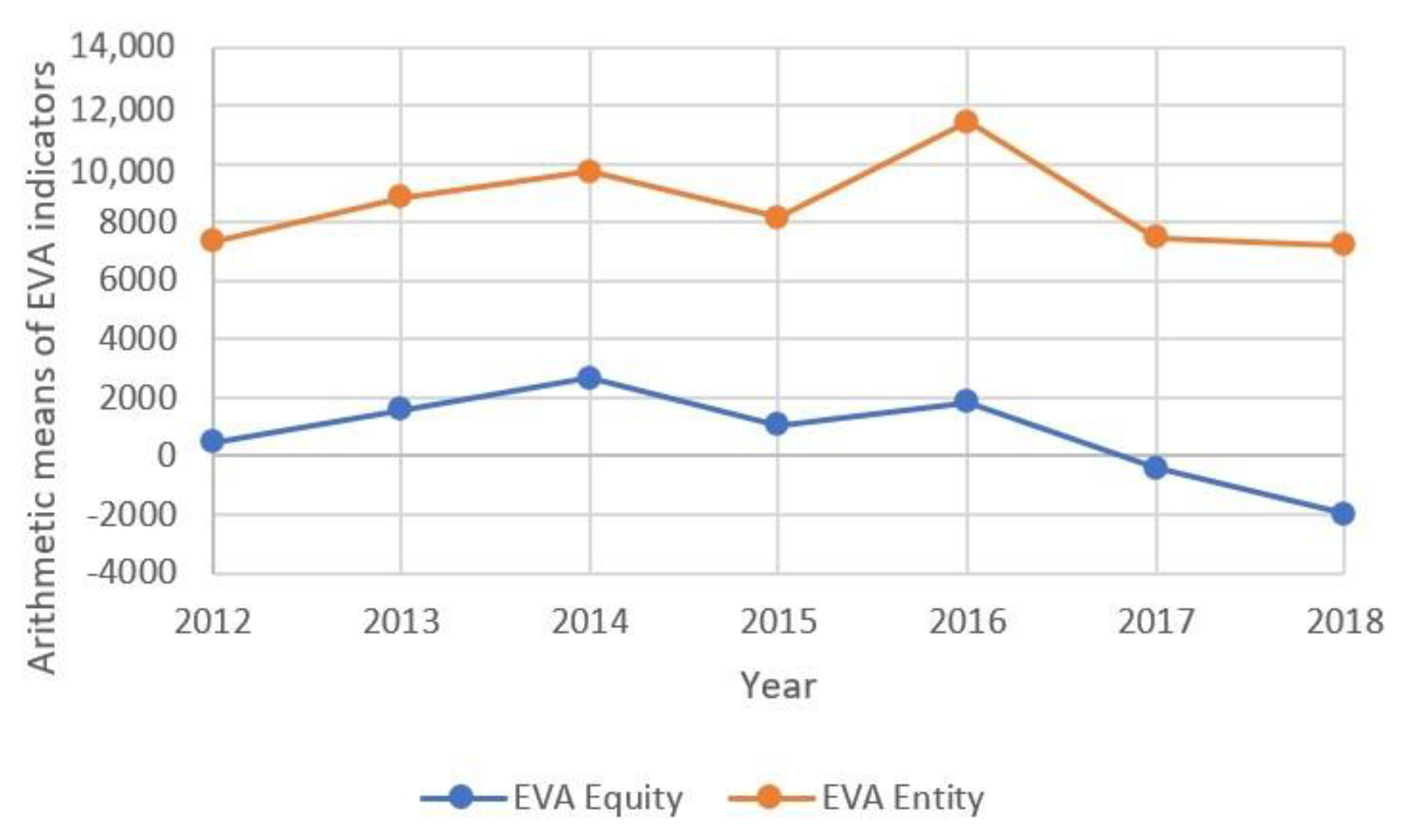
The values of the EVA Equity and EVA Entity indicators were then calculated. All the input and output data for both indicators were subjected to arithmetic means for the respective accounting periods from 2012 to 2018. To illustrate the difference between the EVA Equity and EVA Entity indicators, the EVA Equity and EVA Entity indicators of a model enterprise in the agricultural sector are presented in Figure 1.

Figure 1 shows that the trends for both indicators are almost identical throughout the monitored period. This pattern is analyzed in detail in the discussion section of this article. All the same, the trends slightly diverge from 2017 onwards. In 2017, there was a slightly sharper decrease in the value of the EVA Equity indicator than that of the EVA Entity indicator.

As can be seen in Figure 1, throughout the monitored period, it is evident that the difference between EVA Entity and EVA Equity is positive. This indicates that the credit absorption capacity of the model enterprise in the agricultural sector is good.

These results show that the difference between the EVA Entity and EVA Equity indicators enables us to determine the credit absorption capacity in a specific sector.

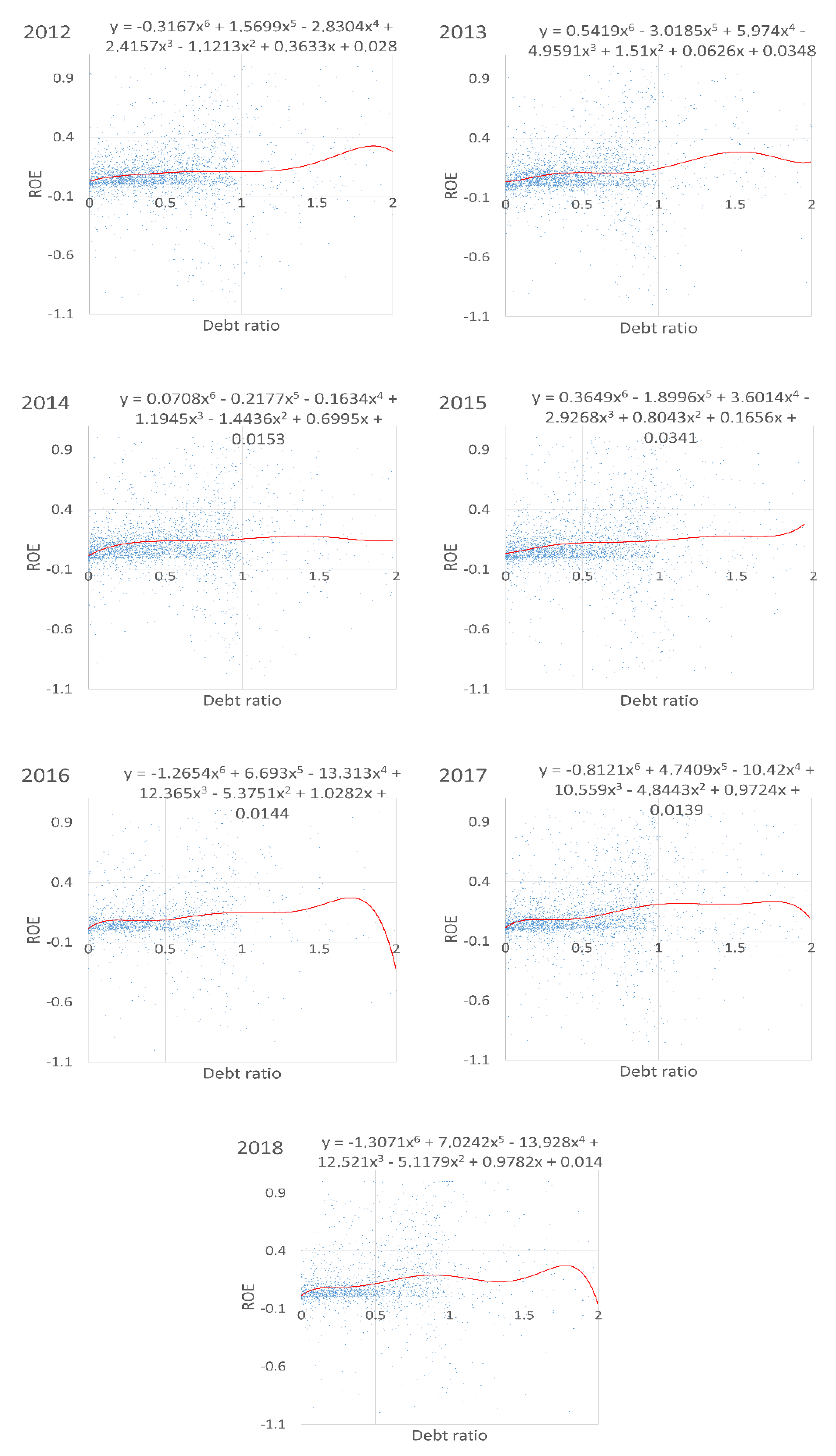
Taking into consideration that the first hypothesis is confirmed, the answer to the second hypothesis was sought. To this end, seven graphs of ROE and the debt ratio of enterprises in the agricultural sector in the dataset were created. Figure 2 illustrates the effect of financial leverage in the monitored years.

Figure 2 shows that financial leverage was highly effective even at different debt ratios throughout the monitored period. In the graphs in Figure 2, the individual points are plotted for all the monitored years based on the relationship between the ROE (axis x) and debt ratio (axis y). The points are fitted with a 6th-degree polynomial trendline. If the polynomial trendline shows an upward tendency, it can be concluded that at these specific intervals of debt ratio, the effect of financial leverage in the agricultural enterprises operating in the CR included in the dataset was positive. The specific intervals linked to the positive effect of financial leverage are presented in

Table 4. Debt ratio intervals of enterprises linked to the positive effect of financial leverage in the agricultural sector.

Year	Debt Ratio	APRC (%)
2012	(0; 0.8>, <1.1; 1.85)	15.92
2013	(0; 0.5>, <0.7; 1.5>, <1.95; 2)	15.03
2014	(0; 1.4>, <1.9; 2)	14.86
2015	(0; 1.45>, <1.65; 2)	12.47
2016	(0; 0.18>, <0.4; 1.0>, <1.2; 1.7)	10.60
2017	(0; 0.2>, <0.35; 1.1>, <1.4; 1.75)	9.14
2018	(0; 0.9>, <1.35; 1.77)	8.97

Source: [51]; the Authors.

. For comparative purposes, the Annual Percentage Rate of Charge (APRC) for the provision of consumer credit by banks operating in the CR for the given year are also presented.

Table 4 shows the debt ratio intervals for enterprises in the agricultural sector linked to the positive effect of financial leverage. In 2012, positive financial leverage effects were achieved with debt ratio intervals of (0; 0.8> and <1.1; 1.85). In 2013, the debt ratio interval was (0; 0.5>, <0.7; 1.5> and <1.95; 2); in the years 2014 and 2015, these were (0; 1.4>, <1.9; 2) and (0; 1.45>, <1.65; 2), respectively. Interestingly, only in the period 2013–2015 were positive financial leverage effects achieved, even with the highest debt ratio (debt ratio = 2). In 2016, positive financial leverage effects were achieved with debt ratio intervals of (0; 0.18>, <0.4; 1.0> and <1.2; 1.7). In 2017, the debt ratio intervals were similar to those in 2016, specifically, (0; 0.2>, <0.35; 1.1> and <1.4; 1.75). In the last year of the monitored period, the intervals were (0; 0.9> a <1.35; 1.77). On the basis of the aforementioned, it can be stated that the maximum debt ratio for maintaining the positive effect of financial leverage in the years 2016–2018 was lower than in the monitored years before this period. It would appear that throughout the monitored period there was a decline in the debt ratio, which has a positive effect on financial leverage. It should also be mentioned that achieving a positive financial leverage effect not only depends on the amount of debt, but also on the ratio of basic earnings to debt interest rate.

The development of the APRC during the monitored period shows that the APRC decreased nearly by half between 2012 and 2018. In this period, debt financing therefore became more accessible to agricultural enterprises.

6. Discussion

A detailed analysis of the input data showed that average equity predominated over the average debt in all the years. This implies that the total capital of the model enterprise in the agricultural sector in the CR is mostly comprised of own resources.

To achieve the objective of this article, two hypotheses were formulated. The first hypothesis focused on whether it is possible to determine credit absorption capacity in the agricultural sector using the values of EVA Entity and EVA Equity; this hypothesis was confirmed in the theoretical background of this article. Based on the theoretical analysis, it can be argued that the differences between the EVA Entity and EVA Equity indicators enables the determination of credit absorption capacity. This result was achieved through the theoretical information in the value derived from the difference between the EVA Entity and EVA Equity indicators. The resulting value therefore contains only information on the debt capital and the operating costs of the enterprise.

The parallel tendency of both EVA indicators during the monitored period can be explained by the fact that the calculation was based on a component that is calculated in the same way in both cases—alternative costs of equity (r_e) calculated using the CAPM model. As this hypothesis was confirmed, we may focus on the second hypothesis, which predicts the positive effect on financial leverage in the agricultural sector.

The second hypothesis was also confirmed. The positive effect of financial leverage used by enterprises in the agricultural sector with different debt ratio intervals was determined by the identified relationship between the debt ratio (axis x) and ROE (axis y). These diagrams were provided with a 6th-degree polynomial curve, which demonstrated the greatest reliability. The debt ratio intervals, whose curve was concave-shaped, showed the positive effect of financial leverage used by the enterprise. In contrast, convex curving showed the negative effect of financial leverage. In the case of the second hypothesis, it was found that it is necessary to determine the debt ratio interval at which the effect of financial leverage is positive. These intervals are presented in Table 4 in the section “Results” of this article. These findings enable the differences between EVA Equity and EVA Entity to be used for determining the optimal credit absorption capacity of enterprises, which can be considered the most important result achieved.

The differences between EVA Equity and EVA Entity indicate that those enterprises operating in the agricultural sector were represented by the aforementioned model enterprise, and are able to absorb various amounts of financial resources when effectively leveraged every year. The highest absorption capacity was determined to be CZK 9.6 million in 2016 compared to the lowest value of CZK 6.88 million recorded in 2012. However, the results clearly show that the credit absorption capacity was incremental within the monitored period. The debt ratio of the model enterprise was 0.49% in 2012–2015, 0.46% in 2016, and did not exceed 0.51% in 2017 and 2018. These debt ratio values are ideal for this model enterprise based on the information about the positive financial leverage effect; it may even be said that, at such debt ratios, the model enterprise is able to maintain the positive effect of financial leverage even when the costs of equity are deduced.

The period 2017 and 2018 is a very specific period for the model enterprise since the EVA Equity indicator showed negative values. In this specific case, the equation has the following form:

$$EV{A}_{Equity}\langle 0\wedge EV{A}_{Entity}-EV{A}_{Equity}\rangle 0$$

(18)

This equation describes the state of the model enterprise, which indicates that the costs of equity (re) are higher than the return on equity (ROE) and that, at the same time, the difference between EVA Entity and EVA Equity is positive. This means that the costs of equity and the costs of the debt capital maintain uneven growth, i.e., the costs of equity show a more rapid increase than those of the debt capital. Business owners therefore face an unreasonably higher risk resulting from the costs of the debt capital, which are higher than necessary. It is therefore recommended to increase the volume of debt capital because this would enable the enterprises to mobilize more financial resources with which to develop their business activities at the same risk level. Additional financial resources could be used to finance the enterprise´s investment in its expansion, facility modernization, and an overall increase in production and profits.

Enterprises could utilize the difference between the EVA Entity and EVA Equity indicators to identify the optimal credit absorption capacity using specific data of a particular enterprise in any sector. Based on the results of the difference between these values, it is possible to optimize the debt ratio so that the highest possible volume of debt capital is achieved to support business activities, thereby maximizing the positive effect of the enterprise´s financial leverage.

Horák et al. [52] set the credit absorption capacity for construction companies. For this purpose, they also used the difference between the EVA Entity and EVA Equity indicators. Based on their results, it is clear that companies operating in the field of construction are not able to increase their value for investors and creditors through loans. In this case, however, conclusions can be drawn confirming the applicability of this procedure to determine the credit absorption capacity in the agricultural sector.

Jang and Tang [53] dealt with the issue of a direct relationship between the positive leverage function and company profitability. From an investor’s point of view, the EVA indicator is also closely related to this. Based on own research, it is therefore possible to confirm the above claims concerning the close relationship between the degree of positive leverage function and company profitability. Memon et al. [54] examined the effect of company cash flow volatility on the variability of leverage function. They found that the positive function of financial leverage as such may be destabilized by the higher volatility of company cash flows. In this article, the relationship between ROE and the debt ratio of an average company operating in the agricultural sector was used to determine the moment of positive leverage function. Mielcarz et al. [55] developed an iterative algorithm to determine the optimal company capital structure so that companies would be able to create value for investors and creditors. In relation to their findings, the algorithm eliminates the inaccuracy of the WACC calculation for the calculation of the EVA Entity indicator. That approach was not used in this article, but in terms of its objective, it cannot be considered as an error that would somehow affect the results achieved. According to Bauer and Bubák [56], it is very important to know the capital structure of companies, since it has a fundamental effect on their value in the eyes of investors. The previously mentioned authors tested the compliance of the theory of optimal capital structure of companies with the potential growth of their value for investors. Such compliance was confirmed, and it was found that companies deviating from the optimal capital structure lose their attractiveness in the eyes of investors. That may also be reflected in calculating EVA indicators. The authors of this article corroborate this point of view and thus confirm it.

7. Conclusions

The submitted text focused on determining the credit absorption capacity of an enterprise by means of differences between the values of EVA Entity and EVA Equity. Hypotheses on using these indicators were formulated on the basis of the theoretical analysis of mathematical operations for both indicators. The difference in the values of EVA Entity and EVA Equity demonstrated that EVA Entity is significantly higher than EVA Equity in all monitored years. This means that enterprises in the agricultural sector in the CR are to some extent dependent on debt capital borrowed from creditors. These indicators can therefore be applied to determine the credit absorption capacity in specific cases in the agricultural sector in the CR. The credit absorption capacity was determined to be CZK 6.88–9.6 million on the basis of the difference between EVA Entity and EVA Equity in the specific sector within the monitored period.

In attempting to verify the second hypothesis, it was found that in the monitored period, the effect of the financial leverage in the agricultural sector is positive only at a specific debt ratio. If the debt ratio is outside this interval, the effect of the financial leverage is otherwise negative, which means that the ratio of total liabilities should be revised. It can therefore be stated that the objective of this article was fully achieved. After all, the research conducted provided the answers to all the posed research questions.

The main contribution of this article is that it put forward a very simple methodological approach that can be applied in practice. This method is applicable across all business sectors (not only the agricultural sector). The application of this methodological approach enables individual enterprises to identify the optimal debt ratio when positively leveraged. This contribution can be considered to be of global importance, since the methodology presented and justified can be used also to determine the optimal debt of foreign enterprises. The agriculture sector of the Czech Republic served only as an example to demonstrate the selected methodology. Determining the optimal debt of a specific sector for other states will be addressed in a following contribution.

However, the results achieved through own research have certain limitations, of which a few are mentioned here. For example, the input data for the calculation obtained from the Damodaran online website are not completely accurate in the case of certain Czech companies. The used database on Czech companies operating in agriculture has also shown certain inaccuracies. Another limitation is the time range of the input dataset, as the research does not include data for 2019, let alone data for 2020, which was not available in any database at the time of writing this article. In general, any research results based on historical data show shortcomings.

With regard to the research limitations, the overall applicability of the methodology proposed is considered good in terms of other sectors as well as in other European countries. Future research will focus on validating this theory using data from another business sector. The results could then be verified using input data of companies operating in the USA, thereby eliminating possible discrepancies of input data received from the Damodaran online website and their application to European companies.