Comparison between Multi-Criteria Decision-Making Methods and Evaluating the Quality of Life at Different Spatial Levels

Abstract

Achieving a good urban form has been a problem since the formation of the earliest cities. The tendency of human populations toward living in urban environments and urbanization has made the quality of life more prominent. This article aimed to calculate the quality of life in an objective way. For this purpose, the technique for order preferences by similarity to ideal solution (TOPSIS), vlseKriterijumsk optimizacija kompromisno resenje (VIKOR), simple additive weighted (SAW), and elimination and choice expressing reality (ELECTRE) have been utilized. Quality of life was assessed at three spatial levels. In this regard, socioeconomic, environmental, and accessibility dimensions were considered. As a result, in the first level of comparison, sub-districts in District 6 were ranked higher than that of District 13. On the second level, for District 6, vicinity sub-districts had higher rankings than the center, and for District 13, sub-districts near the center of the city had higher rankings. In the third level, District 6 had a higher quality of life. The results of the comparison between research methods showed that the SAW method performs better in terms of stability. Based on the results of correlation tables, there was a strong and direct relationship between each pair of methods at three spatial levels. In addition, as the study area became smaller, the similarity between the methods increased.

1. Introduction

Increasing urbanization and the growth of urban areas in cities in developing countries present major challenges for local governments, policy-makers, and urban planners. Studies focusing on quality of life (QoL) help in objectively assessing the urban conditions informing urban policy-makers and planners [1]. Indeed, assessing the quality of life can help policy-makers and professionals with sustainable development in social, economic, environmental, decision-making, and planning aspects. Implementing sustainable development will improve the welfare of the people, which is a very important issue for planners at the macro and micro levels. That is why attention to this issue is very important today.

Quality of life is a multi-dimensional concept that is measured using objective and subjective approaches [2]. While objective dimensions are tangible and measurable observations and indicators that are objective in urban environments and also are measurable using spatial data, subjective dimensions of quality of life are measurements and perception of individuals from their living environment and other aspects associated with this environment [3]. Since the subjective measurement is based on the views of the people, it can be affected by the morale of the people, and its implementation may be far from reality. Therefore, objective measurements must be taken into account so that managers can make more precise plans.

Objective measurement is important because it can help professionals improve the balance between urbanization and the environment, record inequalities, support deprived areas, define priorities, and transfer resources. Additionally, adjusting the various dimensions of quality of life is the basis of policy-makers’ work and decision-making, which plays a vital role in determining the welfare of the people. Therefore, objective measurement was considered in this study.

One problem with measuring the quality of life is the lack of an agreed definition for it. As a result, choosing criteria for measuring the quality of life is difficult. In general, these criteria are built upon factors such as personal environment, public environment, physical environment, atmosphere, and society [4]. According to these issues, quality of life criteria are closely related to the location because in different places, these criteria have different values, and as a result, the quality of life varies from place to place. Therefore, the quality of life of individuals or groups can be determined by the quality of their place of residence. Hence, this paper discusses the quality of life using geospatial information systems because they can manage, compile, store, and display spatial information.

A variety of studies have been conducted around the world on the quality of life. Some studies have examined only limited aspects of quality of life to assess the quality of urban life and have only evaluated one dimension. Zebardast [5] has used housing consolidation, amenities, space, housing quality and basic services, housing durability, and security of tenure in assessing the quality of life in the residential areas in the vicinity of the city of Tehran. In the mentioned paper, factor analysis has been used to identify the effective components in the housing situation of citizens. Banzhaf et al. [6] have used geophysical criteria such as air quality, air temperature, built-up structure, and green space infrastructures in assessing the environmental quality and quality of life. They used qualitative analysis methods and integrated the scales. Chen et al. [7] conducted a study to measure the environmental quality of life using environmental criteria such as educational, health, and recreational facilities, local street networks, compatibility of land use, and building footprint intensity. In their research, they used the principal component analysis (PCA) method. Considering only one dimension is among the limitations of these research works. Because they considered only one dimension, they did not use multi-criteria decision-making methods to weight and combine criteria. Furthermore, in the mentioned research, the evaluation of the quality of life has been done only at the one spatial unit level.

In some studies, spatial criteria were used for evaluating the quality of life. Joseph et al. [8] used some criteria, such as greenness, noise, and air pollution, proximity to water body (including coastal) pollution, open market, cemetery and slum, and the risk of flooding, landslide, and coastal surge. Using experts’ comments, they calculated a specific weight for each layer and provided a qualitative map of the quality of life using weighted averaging and an empirical threshold. Chen et al. [9] developed an objective indicator at the neighborhood spatial scale. They used land-use features for evaluating the quality of life. They used land-use characteristics to categorize neighborhoods. In addition to the spatial dimension, some studies have also considered the temporal dimension of quality of life. Chen and Yu [10] evaluated the spatial-temporal pattern of quality of life. They used socio-economic and meteorological indicators. In this research, although the spatial nature of quality of life has been considered, the evaluations were done only at the one spatial unit level. Additionally, different multi-criteria decision-making methods have not been used to combine the criteria.

Some studies used one multi-criteria decision-making (MCDM) method for evaluating the quality of life. Rinner [11] used some criteria as a bachelor’s degree or higher, employment rate, average individual income, diversity of housing (rented dwellings), immigrants, and the analytical hierarchy process (AHP) method for combining them. Prakash et al. [12] used 10 sub-indices constructed using 54 indicators (49 indicators from the India Census database and 5 remote sensing inputs) in assessing the quality of life in India. They used the AHP method to assign weights to indicators and sub-indices. Furthermore, the geostatistical Moran’s I clustering method was utilized to assign priorities to QoL classes. In his article, Dadashpoor et al. [13] investigated measures such as population density in the region, the share of the city units on service capacity, neighborhood impact, and accessibility alongside the AHP method for the purpose of data integration and used the Gini coefficient to assess the inequality. Bhatti et al. [14] used data related to physical health, psychological and social relationships, environment (natural and built), economic conditions and development, and access to facilities and services in assessing the quality of life. The mentioned paper utilized the AHP method for the weighting process. One of the shortcomings in these research works is the lack of use of other multi-criteria decision-making methods that may be more efficient. Therefore, the optimal method cannot be chosen. Moreover, spatial metrics have been less taken into account. In addition, the evaluations were done only at the one spatial unit level.

Some studies used several MCDM methods for evaluating the quality of life. Gonzalez et al. [15] used indicators for assessing the quality of life such as consumption-related aspects, social services, housing, transport, environment, labor market, health, culture and leisure, education, and security. They have used the Data Envelopment Analysis (DEA) methodology and the developed Value Efficiency Analysis (VEA) methodology to aggregate the information and derive an index of the quality of urban life. Özdemir Işık and Demir [16], in their study, investigated the effects of existing coast characteristics and historical-cultural structure changes in recreation and tourism on the quality of life with respect to the Trabzon coastline in Turkey to increase the quality of life of citizens. The AHP method for the main criteria, while the ELECTRE method was used for the sub-criteria; in fact, a combination of multi-criteria decision-making methods was created to rank all the indicators. Kaklauskas et al. [17] have considered the quality of life as an indicator along with other indicators of a sustainable city in the study of urban sustainability. The purpose of the mentioned paper is to compare several alternative methods for assessing the urban quality of life. In this regard, the Quality of Life Index (QLI) and INVAR methods had been used. One of the drawbacks of these research works is the lack of evaluation quality of life in the different spatial units. In addition, the best decision-making method in terms of stability (stability of the method under the same conditions) in the field of quality of life has not been selected.

Generally, the majority of research has some disadvantages. (1) The quality of life has not been studied simultaneously at different spatial units and on small scales, while it becomes increasingly important to maintain similar levels of QoL in our growing urban centers [11]. (2) Different methods of decision-making have not been used, not allowing to select the most efficient ones. (3) The best decision-making method in terms of stability has not been chosen. (4) Most researchers have used AHP in the quality-of-life literature, which may not be efficient, so other methods should be considered. (5) Some researchers have not used effective spatial criteria. (6) Most researchers have used only one method to calculate the quality of life. Lastly, (7) some researchers have used one dimension to calculate the quality of life, the results of which may not be appropriate because the quality of life is a multi-dimensional concept. Therefore, this research seeks to resolve the gaps existing in previous research.

The main objective of this article is to evaluate the quality of life from an objective perspective. In this regard, there are other objectives defined as (1) ranking and comparing the quality of life in the sub-districts of two districts in Tehran, namely District 6 and District 13 (24 sub-districts); (2) ranking and comparing the quality of life within sub-districts of each district separately; (3) comparing the quality of life in Tehran’s District 6 and 13; and (4) conducting a comparison among multi-criteria decision-making methods in the calculation of quality of life. The latter objective itself consists of three parts: (a) Analysis of the results of calculating the quality of life by different methods; (b) computing the correlation among the methods; and (c) measuring the stability of the methods (providing a quantitative indicator). The dimensions considered for evaluation in this study are the (1) socio-economic dimension, (2) environmental dimension, and (3) accessibility to urban facilities and services. There are some complications in the way of achieving these goals. For instance, which decision-making method is to be used for the objective assessment of the quality of life? Furthermore, what criteria are to be considered for this assessment? For this purpose, a study was conducted on the previous research to provide a general summary of the criteria and methods used to calculate the quality of life. The most appropriate criteria and methods were chosen. Quality of life was measured based on each criterion and then integrated with multi-criteria decision-making methods. With regards to the quality of life, many papers have used the AHP (analytical hierarchy process) method for data integration, which may not be efficient, so other methods need to be checked. Among these methods, SAW (simple additive weighted), TOPSIS (technique for order preferences by similarity to ideal solution), VIKOR (vlseKriterijumsk optimizacija kompromisno resenje), and ELECTRE (elimination and choice expressing reality) are used and compared for simplicity, ease, and the possibility of rating of options. Finally, comparisons were made in the ranking of areas with the different decision-making methods and in different spatial units and among the decision-making methods. These comparisons will provide better results and more effective solutions. The more appropriate and realistic the results are, the more accurate decisions and plans are made. One of the most important contributions of this research is analysis at a different spatial level, because after examining the quality of life at each level, a comprehensive program can be achieved by combining them. This issue has received less attention in the quality of life. Furthermore, the numerical analysis of this research has been strengthened by comparing several multi-criteria decision-making methods. This can affect the results.

The current research has been set up in five sections. The first section is an introduction to the quality of life. The second part introduces the case study. The third part presents the materials and methods. The fourth part is the results and discussion, and finally, the fifth part discusses the conclusion and future suggestions.

2. Case Study

According to the latest census (2016), Tehran is the most populous city in Iran. Tehran has problems such as lack of urban green space, noise and air pollution, weakness in the transportation system, lack of service, welfare, public spaces, physical deterioration of the area, especially in old neighborhoods, and low-income levels of residents. Due to these cases, choosing this city is a priority to assess the quality of life. In Tehran, most traffic takes place in the city center, and a large number of people pass through Tehran’s District 6 every day. Additionally, District 13 is actually a longitudinal area that can have a good diversity in terms of quality of life. Therefore, Districts 6 and 13 are a good choice for assessing the quality of life.

This research focused on Districts 6 and 13 in the city of Tehran. District 6 is located in downtown of Tehran, bound to the north by Hemmat Highway, to the west by Chamran highway, to the east by Modarres Highway and Mofatheh Street, and also to the south by Enghelab Street. The district has an area of 21.1345 km² and 11 sub-districts.

District 13 is located in the east of Tehran. It is bound to the north by Damavand Street, to the east by Yasini Highway, to the south by Piroozi Street, and to the west by the 17th Shahrivar Street. Its area is about 1283 hectares. District 13 is divided into 13 sub-districts, according to the Tehran City Council. The 2011 census data of the Iranian Statistics Center were used to calculate the socio-economic dimension of quality of life. The Landsat 8 satellite imagery was used to calculate the greenness. Moreover, the Landsat 8 satellite imagery was used to calculate the land surface temperature. The air quality control centers of Tehran data are used for the calculation of air pollution. The quality control stations inside the case study and its surroundings are used. Land use layers from Tehran’s municipality and road network layers from the Traffic Control Company were used to calculate the noise pollution and accessibility to the urban facilities. In Figure 1, the location of two districts in the city is specified.

3. Methodology

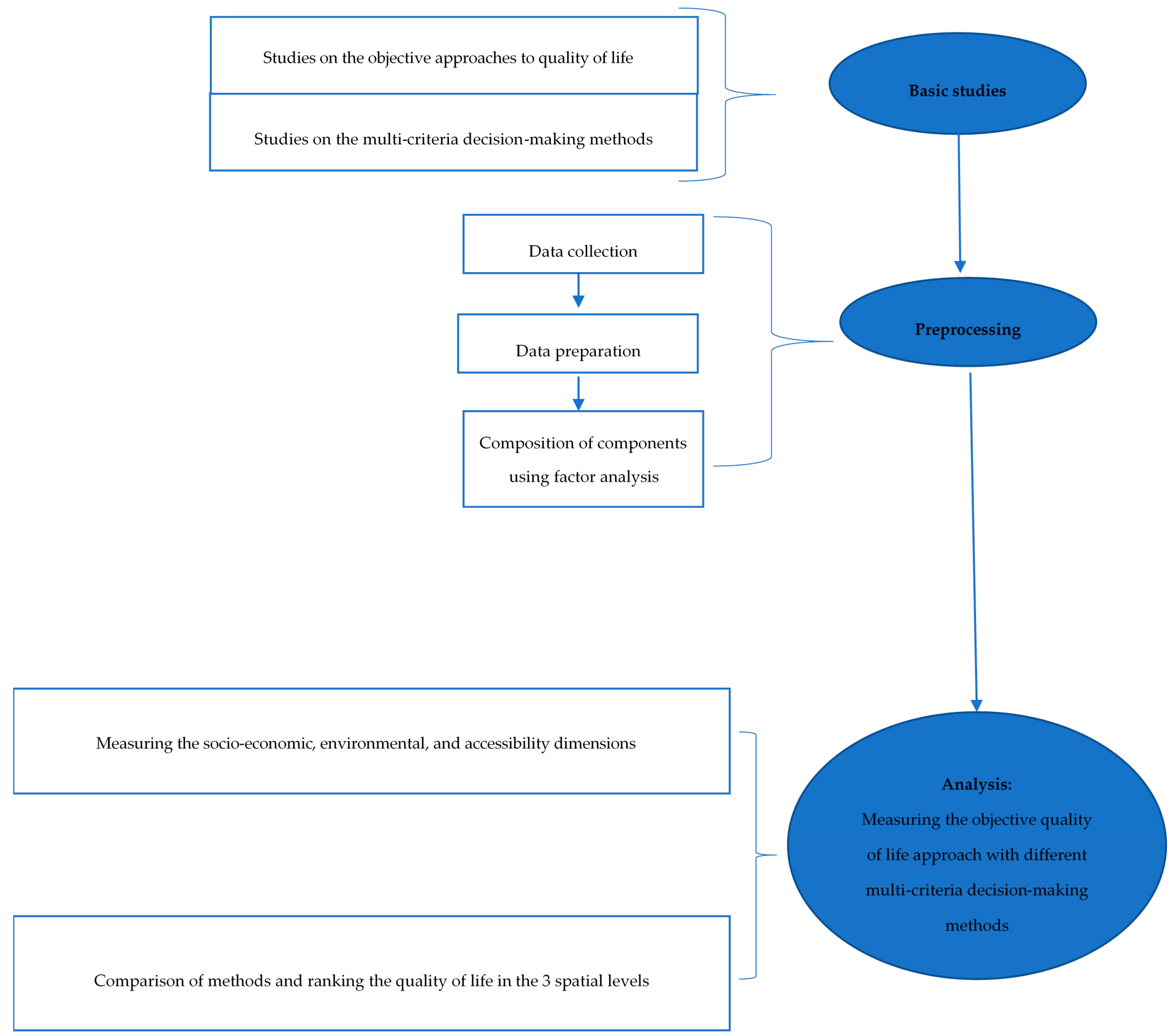
The purpose of this article is to evaluate the quality of life from an objective perspective. The dimensions to be considered for this assessment are (1) socio-economic dimension, (2) environmental dimension, and (3) accessibility to urban facilities and services. For this purpose, the 2011 census data of the Iranian Statistical Center, satellite images from Landsat 8, land use layout, and traffic control information in Tehran have been used. There are some problems to achieve the purpose of this study, including the methodology used to evaluate the quality of life objectively and what criteria to consider for this assessment. To this end, a preliminary study was undertaken to provide a general summary of the criteria and methods to calculate the quality of life. Then, the most appropriate criteria and methods were selected. After that, preprocessing has been done. In this regard, the first data collection has been done. After that, data preprocessing and then the composition of components have been done using factor analysis. The socio-economic dimension of quality of life was measured using factor analysis. The suitability of data for factor analysis was evaluated using the KMO coefficient and the Bartlett test. The environmental dimension of quality of life was measured using 4 indicators: (1) Greenness index; (2) land surface temperature index; (3) air pollution index; and (4) noise pollution index. The accessibility dimension of quality of life was measured using 9 land uses: (1) Park, (2) fire station, (3) gas station, (4) BRT (Bus Rapid Transit) station, (5) urban bus station, (6) metro station, (7) mosque, (8) hospital, (9) hospital and clinic.

Quality of life was measured in terms of each criterion, and the results were combined with multi-criteria decision-making methods, including SAW, TOPSIS, VIKOR, and ELECTRE. Finally, comparisons were made in the ranking of areas among different decision-making methods and in different spatial units. Quality of life was assessed at three spatial levels. The first level was a comparison between sub-districts of the two districts. The second level was a comparison between the sub-districts of one district, and the last level is a comparison of the two districts. In each of these three levels, a comparison has been made between the integration methods. The correlation between the integration methods was computed. In addition, the methods’ stability indices were presented. A summary of the workflow of the paper is presented in Figure 2. The evaluation of each research dimension and the combination of their dimensions using multi-criteria decision-making (MCDM) methods are examined in more detail below.

3.1. The Evaluation of the Three Research Dimensions

In this section, the evaluation of each research dimension is examined in more detail below. To the best of our knowledge, not only did previous studies fail to provide a complete list of the quality of life criteria, but each of them determined the criteria according to available data and specific purpose. The existing criteria in the previous studies are summarized in

Table 1. Summarizing the quality of life criteria of previous studies.

Researchers Name and Year of Research	Quality of Life Criteria	Method Used
Rinner [11]	Academic degree (bachelor’s degree or higher), employment rate, average individual income, diversity of housing (rented dwellings), immigrants	Using the AHP method for weighting
Zebardast [5]	Housing consolidation, housing amenities, housing space, housing quality, basic housing services, housing durability, and security of tenure	Using factor analysis to identify effective components
González et al. [15]	Consumption-related aspects, social services, housing, transport, environment, labor market, health, culture and leisure, education and security	The use of the Data Envelopment Analysis (DEA) method and the developed Value Efficiency Analysis (VEA) method to aggregate the information and to derive an index of the quality of urban life
Banzhaf et al. [6]	Geophysical criteria such as air quality, air temperature, built-up structures and green space infrastructures	Using qualitative analysis methods and integrated scales
Joseph et al. [8]	Greenness, noise and air pollution, proximity to water body (including coastal) pollution, open market, cemetery and slum, and the risk of flooding, landslide and coastal surge	Using experts’ comments, determining a weight for each layer, weighted averaging and defining an empirical threshold to provide a qualitative map of the quality of life
Chen and Si Chen [7]	Environmental criteria such as educational, health, and recreational facilities, local street networks, land use compatibility, and building footprint intensity	Using the Principal Component Analysis (PCA) method
Prakash et al. [12]	The use of 10 sub-indices constructed using 54 indicators (49 indicators from India census database and 5 remote sensing inputs)	Using the AHP method to allocate weights to indicators and sub-indices and the geostatistical Moran’s I clustering method to assign priorities to QoL classes
Dadashpoor et al. [13]	The population density in the region, the share of the city units on service capacity, neighborhood impact, accessibility	Using the AHP method for data integration and the use of Gini coefficient to assess inequality
Özdemir Işık and Demir [16]	Existing coast characteristics, historical-cultural changes in recreation and tourism in the Trabzon coastline	Using the AHP method for the criteria and using the ELECTRE method for the sub-criteria, in fact, the combination of multi-criteria decision-making methods to the ranking of indicators
Bhatti et al. [14]	Physical health, psychological and social relationships, environment (natural and built), economic conditions and development, and accessibility to facilities and services	Using the AHP method in weighting
Nanor et al. [1]	Demographics (population-dependent), economics, availability of basic amenities in a house, health, housing, and neighborhood safety	Using factor analysis method
Kaklauskas et al. [17]	Quality of Life Index (QLI) indicators	Using the QLI and INVAR methods

. The most appropriate and integrated criteria are selected in this study. These criteria constitute the three main dimensions of research.

3.1.1. Socio-Economic Dimension of Quality of Life

Studies have shown that quality of life has a significant relationship with socio-economic variables [11]. The 2011 census data of the Iranian Statistics Center were used to calculate these variables. In this study, 22 variables were considered at first, but after the analyses, 18 variables were selected. The selection of variables in this section is based on relevant studies as well as the availability and innovation of the research. After selecting each variable, the percentage of the selected variable relative to other variables is calculated. Then, for the purpose of analysis of the dataset, factor analysis is used.

Factor analysis is a statistical method aiming to reduce the volume of data and determine the most important and effective variables in the analysis, as well as to find the hidden structure within the data. In this method, it is necessary to examine the suitability of the data for entering the factor analysis. In this regard, one of the methods for choosing the appropriate variable is using the correlation matrix. First, the correlation matrix between the variables is calculated. It shows whether a relationship between variables exists, causing the formation of clusters of correlated and uncorrelated variables. Then, variables that have no significant correlation with any other variables are excluded from the analysis. In other words, the method determines how some variables are related to a smaller number of factors (non-observed variables).

Another method for determining the suitability of data for factor analysis is to use the KMO coefficient and the Bartlett test, with KMO always fluctuating between zero and one. If the KMO value is less than 0.5, the data are not suitable for factor analysis, and if the value is between 0.5 and 0.7, it can be used with caution in the factor analysis. However, if the value is greater than 0.7, the data correlation will be appropriate for factor analysis. Bartlett’s test examines the hypothesis that the observed correlation matrix belongs to a population with uncorrelated variables. In fact, Bartlett’s test is the minimum condition for conducting factor analysis. The next step is to extract the components that explain the maximum variance in the data. In this paper, principal component analysis has been used. Here, an eigenvalue criterion was used to determine the components. Components with an eigenvalue of greater than 1 are considered significant components.

In the next step, the matrix of components and variables is interpreted. The values of this matrix represent the relationship between variables and components that are known as the factor loadings in this research. To express and interpret the intensity of the relationship between variables and components, based on [18], loadings of 0.71 and higher are excellent, within 0.63–0.71 are known as very good, within 0.55–0.63 are known as good, within 0.45–0.55 are considered relatively good, and within 0.33–0.45 are weak.

Finally, the final indicator of the socio-economic dimension of quality of life was obtained after the standardization of each component with the help of Equation (1) [19].

$$S_{QoL}={\displaystyle \sum }_1^n{F}_i*W_i$$

(1)

where $S_{QoL}$ is the final index of the socio-economic dimension of quality of life, n is the number of components, F_i is the specific component i, and W_i is the percentage of variance explained by the i-th component.

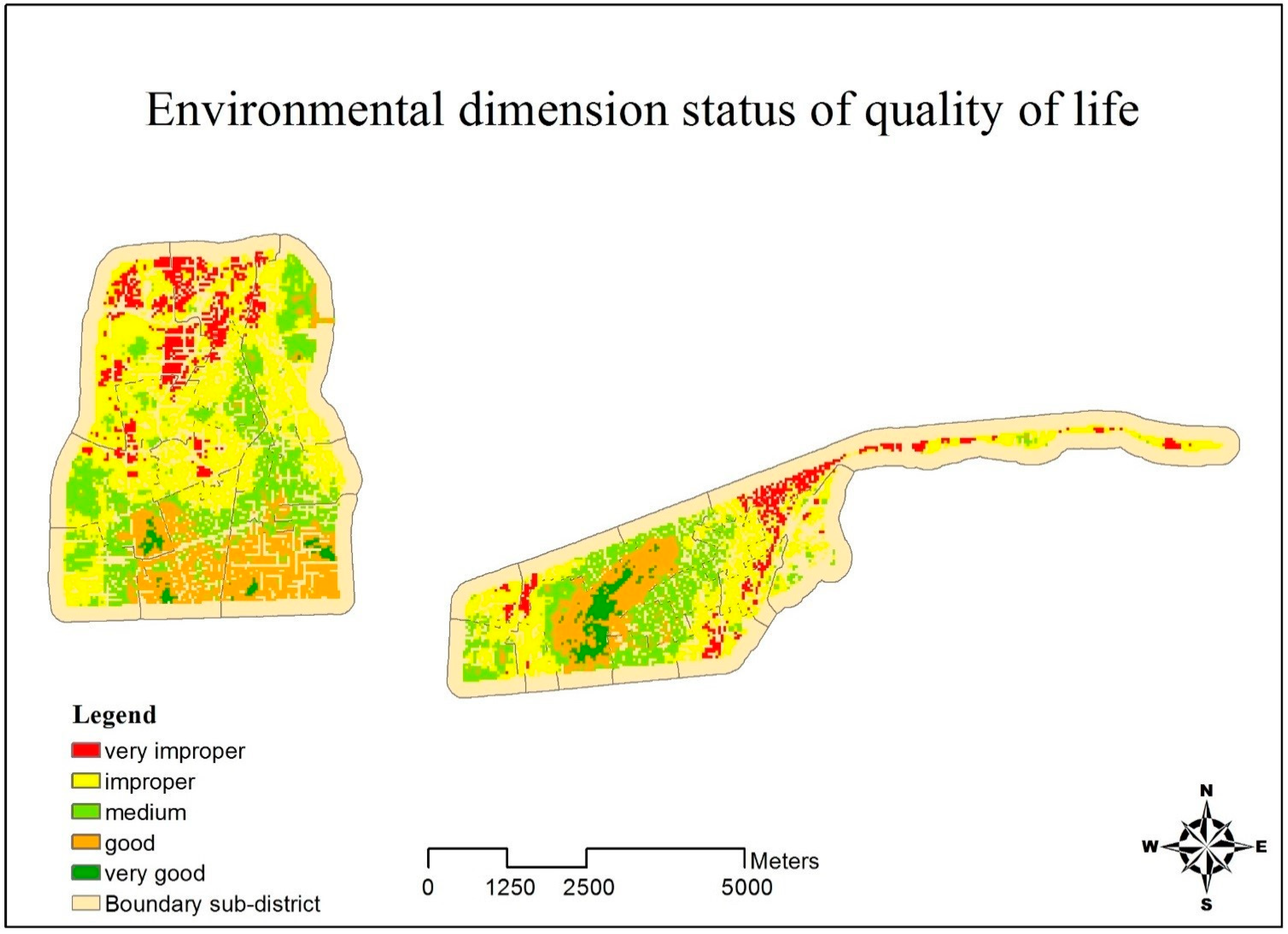
3.1.2. Environmental Dimension of Quality of Life

Since this dimension depends on many factors, those available factors that are referred to in previous studies have been taken into account in this study [6]. The environmental dimension indicators are spatial-temporal. For the air pollution, the average monthly measurement of 2017 was used, and for temperature, greenness, and noise pollution, the temporal variations were neglected. This dimension of quality of life is obtained from by overlapping the results of the following four stages.

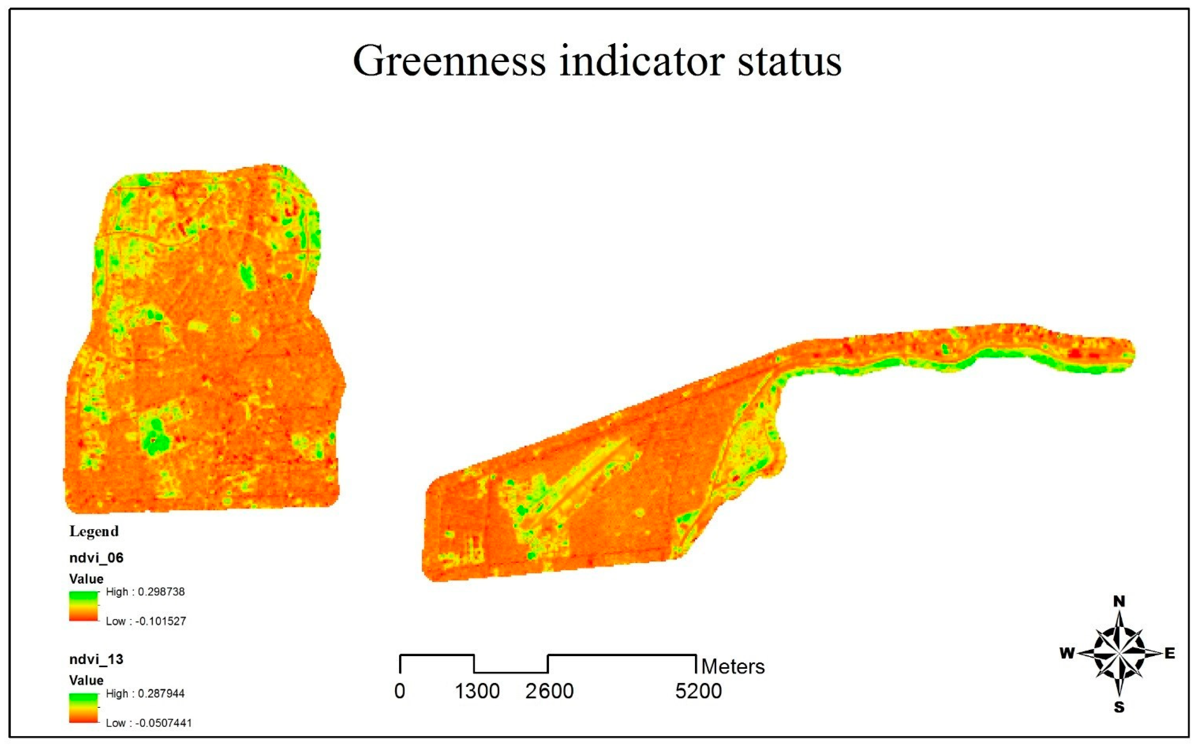
Calculation of Greenness

The Landsat 8 satellite imagery was used to calculate the greenness on 17 February 2017. The NDVI greenness index was obtained from OLI Bands 4 and 5. The Band 4 works in red (R) and Band 5 works in the infrared (NIR) range of the spectrum. The range of NDVI is between −1 and +1. The closer to +1, the greater the greenness density. Equation (2) was used to calculate this index [20].

$$NDVI=\frac{NIR-R}{NIR+R}$$

(2)

Calculation of Land Surface Temperature

First, the radiance values of the two TIR sensor bands 10 and 11 are extracted from satellite images, according to Equation (3) [21].

$$L_{\lambda }=(M_L*Q_{cal})+A_L$$

(3)

where L_λ is a spectral radiance (top of atmosphere), M_L, band-specific multiplicative rescaling factor from the metadata (RADIANCE_MULT_BAND_x, where x is the band number), Q_cal is quantized and calibrated standard product pixel values (Digital Number), and A_L is band-specific additive rescaling factor from the metadata (RADIANCE_ADD_BAND_x, where x is the band number). M_L and A_L in the metadata file associated with the Landsat 8 image.

Then, the proportion of vegetation (P_v) and earth surface emissivity (E) is obtained from Equations (4) and (5) [21], respectively.

$$Pv={\left(\frac{NDVI-NDV{I}_{min}}{NDV{I}_{max}-NDV{I}_{min}}\right)}^2$$

(4)

In Equation (4) [21], NDVI, NDVI_min, and NDVI_max are the minimum and maximum greenness index, respectively.

$$E=\left(0.004*Pv\right)+0.986$$

(5)

Finally, land surface temperature (LST) was calculated using Equations (6) and (7) [21].

$$BT=\frac{k_2}{ln\left(\frac{k_1}{L_{\lambda }}+1\right)}$$

(6)

where BT is the top of atmosphere brightness temperature, k₁ is band-specific thermal conversion constant from the metadata (K1_CONSTANT_BAND_x, where x is the thermal band number), and k₂ is the band-specific thermal conversion constant from the metadata (K2_CONSTANT_BAND_x, where x is the thermal band number), the thermal conversion constants (for the two thermal bands 10 and 11 in the satellite image metadata file), and L_λ is the spectral radiance (top of atmosphere).

$$LST=\frac{BT}{1}+\left(w*\frac{BT}{p}*ln\left(E\right)\right)$$

(7)

where BT is the top of atmosphere brightness temperature, w is the wavelength of emitted radiance, p is 14,380 and E is the land surface emissivity.

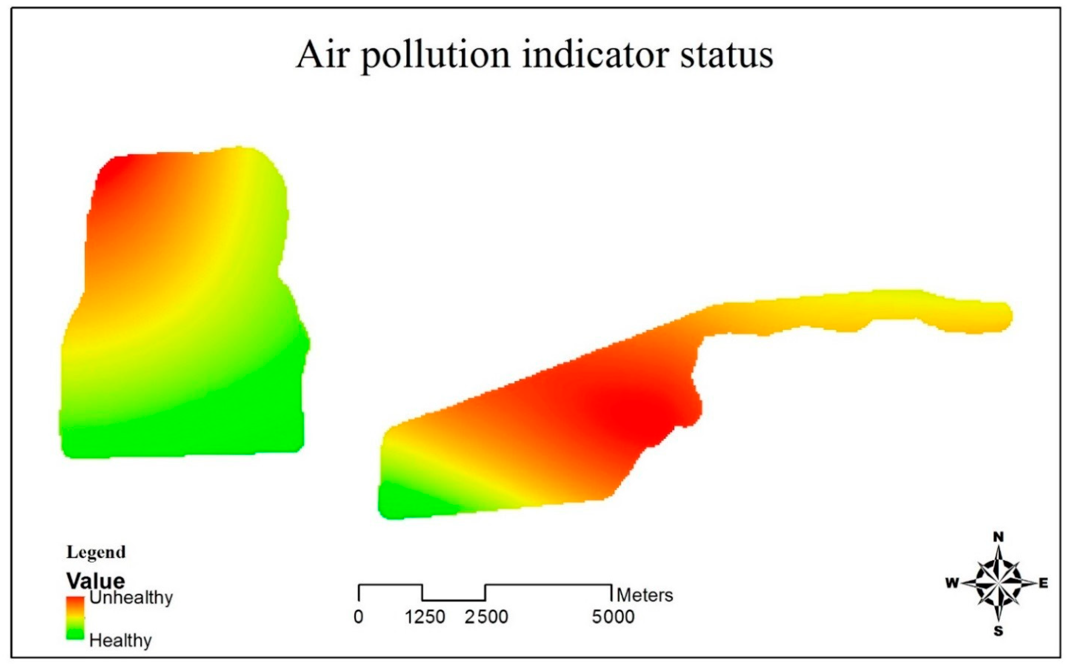
Calculation of Air Pollution

In this section, the air quality control center’s data and, in particular, the Air Quality Index (AQI), including CO, O₃, NO₂, SO₂, Pm₁₀, and Pm_2.5 pollutants, have been used. The quality control stations inside the study area and its surroundings include 7 stations: (1) Crisis Headquarters—District 7; (2) Municipality—District 4; (3) Municipality—District 10; (4) Mahallati Highway—District 14; (5) Piroozi—District 13; (6) Tarbiat Modarres—District 6; (7) Sharif-District 2.

For each station, average values of AQI for January 2017 (due to the peak air pollution in this month) were calculated. Then, the area covered by these 7 stations was placed within a polygon so that interpolation and determination of the amount of contamination for each point becomes possible.

Calculation of Noise Pollution

In the noise pollution section, land use data, including educational, medical, residential, recreational, commercial, and commercial-residential were used. Furthermore, the road network layer, provided by the Traffic Control Company, including highways, main streets, and adjacent streets, was used. In this section, the population density layer was also calculated from the residential blocks. Finally, all layers were converted to raster format and normalized between zero and one. According to

Table 2. Weights of the criteria and sub-criteria in the noise pollution map [22].

Criterion	Weight	Sub-Criterion	Weight of Sub-Criterion	Final Weight
road network	0.724	highway	0.678	0.497
		main street	0.244	0.177
		adjacent street	0.069	0.05
Land use	0.192	commercial	0.423	0.081
		commercial-residential	0.298	0.057
		educational	0.117	0.022
		recreational	0.078	0.015
		medical	0.051	0.01
		residential	0.035	0.007
population density	0.083	-	1	0.083
			Total	1

, in which the hierarchical weights of the layers have come from previous studies, each layer is multiplied by its weight and the noise pollution layer is calculated according to the available data.

3.1.3. Accessibility to Urban Facilities and Services as a Dimension of Quality of Life

According to the roads network layer of Tehran Traffic Control Company, using network analysis, the service area was obtained at the level of each block of statistical data for each land use, and an aggregation method was used to calculate the accessibility. Finally, for each land use, according to Equation (8), weighted averaging was performed. The reason for using this method lies in its simplicity. In this section, there are two important points that distinguish this research. First, the level of accessibility was calculated at a very small spatial unit level (statistical blocks). Second, the service areas of different land uses are not limited to the official areas of the municipality (sub-districts and districts), i.e., the impact of other areas on accessibility is considered. As a result, the value of accessibility criteria will be more accurate.

$$D={\displaystyle \sum }_1^n\frac{\left(y*x_n\right)}{k}$$

(8)

In this formula, D is the weighted population average of accesses to the sub-district, n is the number of sub-districts, y is the population of each block, k is the population of each sub-district, and x is the number of accesses to each land use.

3.2. Combining the Research Dimensions Using Multi-Criteria Decision-Making (MCDM) Methods

Finally, the results obtained from the three dimensions were combined using SAW, VIKOR, TOPSIS, and ELECTRE methods, and the sub-districts were ranked at different spatial levels. Then, comparisons were made between rankings and between methods at different spatial levels. In the following, a review of the literature and the theoretical basics of multi-criteria decision-making methods will be described.

3.2.1. Relevant Literature and Theoretical Basis of Multi-Criteria Decision-Making (MCDM) Methods

Multi-criteria decision-making (MCDM) methods are successfully applied in various fields. Many studies have used multi-criteria decision-making methods to solve decision-making problems. Liu et al. [23] used VIKOR for prioritizing municipal solid waste sites. Gigovic et al. [24] used TOPSIS and VIKOR for ranking ammunition depots sites. Kumar et al. [25] used ELECRE for hospital site selection. Erbas et al. [26] used TOPSIS for ranking potential electric vehicle charging stations (EVCS) sites. Rahim et al. [27] used the TOPSIS ranking method to select the best employees using the relevant criteria. The results of this study showed that the use of the TOPSIS method could improve the decision-making process. Ozkaya et al. [28] used TOPSIS, VIKOR, PROMETHEE I-II, ARAS, COPRAS, MULTIMOORA, ELECTRE, and SAW methods to compare and rank 40 countries in terms of science, technology and innovation indicators. Sałabun et al. [29] examined the methods of TOPSIS, VIKOR, COPRAS, and PROMETHEE II and tested 4 selected methods for multi-criteria analysis. The results of this study showed that the final rankings obtained from the 4 MCDA methods are similar. Therefore, it is necessary to study and compare the performance of these methods in different areas. Additionally, to solve the MCDM problems, there are many methods that are divided into two main categories, compensatory and non-compensatory. In compensatory methods, weaknesses in an index are compensated in other indices. In this research, four compensatory methods have been used: (1) The VIKOR method is expressed as a consensus solution and multi-criteria optimization approach. (2) The TOPSIS method utilizes the concept of similarity to the ideal option. It is commonly used to solve multi-criteria problems due to its ease of use [30,31]. (3) The SAW method is a simplified weighted average. (4) The ELECTRE method is based on paired comparisons between options for each of the criteria [32]. Generally, multi-criteria decision-making methods have been used in various fields [33,34,35,36]. Therefore, based on the unique features of these 4 methods, these four methods have been selected. The following is a description of each one.

VIKOR Method

VIKOR’s methodology has been developed for multi-criteria optimization of complex systems, focused on ranking and selecting a set of options, and determining agreed solutions to a problem with contradictory criteria that can help decision-makers reach a final decision. Here, the agreed solution is a possible solution that is the closest to the ideal solution. The agreement is achieved by mutual concessions.

This methodology is a multi-criteria ranking index based on a certain amount of closeness to an ideal solution [37,38]. The VIKOR method is a useful tool in multi-criteria decision-making, especially in a situations where the decision-maker is unable to express the priorities at the beginning of design of the system [39].

VIKOR’s method focuses on ranking and selecting from a set of different options and determines compromise solutions for a problem with incompatible criteria. In this method, decision-makers can reach the final decision. The compromise answer may be the closest to the ideal answer, and the compromise is an agreement on two-way exchanges. The advantage of the VIKOR method can determine a compromise solution to reflect the attitude of most decision-makers [40,41]. The advantage of using the VIKOR method in the present study is that it does not rely solely on personal judgments and uses valid statistics and data.

The steps of the VIKOR method are as follows:

• Determine the best (f_i^*) and worst (f_i⁻) values in all criteria based on Equations (9) and (10) [30].

  $$f_j^{*}=\underset{i}{\max }{f}_{ij}, f_j^{-}=\underset{i}{\min }{f}_{ij}$$

  (9)

  $$f_j^{*}=\underset{i}{\min }{f}_{ij}, f_j^{-}=\underset{i}{\max }{f}_{ij }$$

  (10)
• S_i and R_i are calculated using Equations (11) and (12). w_j is the weight of the criteria that determines their relative importance [30].

  $$S_i={{\displaystyle \sum }}_{j=1}^n{w}_j\left(f_j^{*}-f_{ij}\right)/\left(f_j^{*}-f_j^{-}\right)$$

  (11)

  $$R_i=\underset{j}{\max }\left[w_j\left(f_j^{*}-f_{ij}\right)/\left(f_j^{*}-f_j^{-}\right)\right]$$

  (12)
• Calculate the value of Q_i using Equation (13) [30].

  $$Q_i=\frac{v\left(S_i-S^{*}\right)}{S^{-}-S^{*}}+\left(1-v\right)\left(R_i-R^{*}\right)/\left(R^{-}-R^{*}\right)$$

  (13)
• The value of v in this regard is the weight for applying the maximum group tool strategy (Equations (14) and (15)) [30].

  $$S^{*}=mi{n}_i{S}_i, S^{*}=mi{n}_i{S}_i$$

  (14)

  $$R^{*}=mi{n}_i{R}_i, R^{*}=ma{x}_i{R}_i$$

  (15)
• At this stage, the ranking of alternatives is done. For this purpose, the values are arranged in descending order and lower values indicate the desirability of more alternatives [30].

TOPSIS Method

The basic logic of the TOPSIS method (the method of arranging preferences in terms of the similarity to the ideal solution) is to define ideal positive and negative solutions based on the shortest distance to an ideal solution [42]. The ideal positive and negative solutions are hypothetical solutions in which all the values of the index are similar to the maximum and minimum index values in the database, respectively [43].

In short, a positive ideal solution is a combination of the best available values of the criteria and the ideal negative solution included the worst available values of the criteria [29]. In practice, TOPSIS is used in MCDM to solve the selection and evaluation in problems with a limited number of options [44,45]. The TOPSIS method, similarly to the VIKOR method, is based on distance measurements [31]. This technique is such that the type of indicators can be included in the model in terms of positive or negative impact on the decision-making goal, and the weights and degrees of importance of each indicator can be entered into the model. Quantitative and qualitative criteria are also involved in the evaluation simultaneously, and a significant number of criteria and options are considered. This method is applied easily and quickly. This method is a compensatory method, and the weight of all options and criteria is involved in decision-making [46]. The steps of the TOPSIS method are summarized as follows:

• The decision matrix becomes a normalized matrix, using Equation (16).

  $$n_{ij}=\frac{r_{ij}}{\sqrt{{{\displaystyle \sum }}_{i=1}^m{r}_{ij}^2}}$$

  (16)
• Using Equation (17), the V_ij the weighted normalized decision matrix is obtained. In this step, the normalized matrix is multiplied by the diagonal matrix of the weights [29].

  $$v_{ij}=w_i{r}_{ij}$$

  (17)
• The positive ideal solution and the negative ideal solution at this stage are determined using Equations (18) and (19) [29].

  $$v_j^{+}=\left\{v_1^{+}, v_2^{+}, \dots , v_n^{+}\right\}=\{ma{x}_j\left(v_{ij}\right)$$

  (18)

  $$v_j^{-}=\left\{v_1^{-}, v_2^{-}, \dots , v_n^{-}\right\}=\{mi{n}_j\left(v_{ij}\right)$$

  (19)
• The distance of each criterion to the positive and negative ideals is obtained using Equations (20) and (21) [29].

  $$D_i^{+}=\sqrt{{{\displaystyle \sum }}_{j=1}^n{\left(v_{ij}-v_j^{+}\right)}^2}$$

  (20)

  $$D_i^{-}=\sqrt{{{\displaystyle \sum }}_{j=1}^n{\left(v_{ij}-v_j^{-}\right)}^2}$$

  (21)
• Determining the relative proximity (C_i) of a criterion to the optimal solution using Equation (22). Based on the descending order of C_i, the criterions can be ranked [29].

  $$C_i=\frac{D_i^{-}}{D_i^{-}+D_i^{+}}$$

  (22)

SAW Method

The SAW method is among the most often used techniques for resolving spatial decision-making problems. The decision-maker directly assigns relative importance (weights) to each attribute. A total score is then obtained for each alternative (land unit) by multiplying the importance weight assigned for each attribute by the scaled value given to the alternative for that attribute and summing the products overall attributes. The alternative with the highest overall score is chosen [47].

Calculation of this method is simple and can be done without the help of complex computer programs [48]. The SAW method is the best-known and most-adopted MCDM model for only considering the weights of criteria and the additive form. Because of its simplicity, it is the most popular method in MCDM problems. SAW method’s advantages are its simplicity and its ability to do the assessment more precisely because it is based on predetermined criteria and preference weights [49]. In the SAW method, unlike other methods, there are no positive or negative factors in choosing the optimal option. The decision-making function of this decision-making technique is linear, and the collectivity of the features is guaranteed.

The SAW method is applicable in the following orde:

• Quantifying the decision matrix.

  $$r_{ij}=\frac{x_{ij}}{max{X}_{ij}} i=1, \dots , m;j=1, \dots , n$$

  (23)
• Linear normalized of decision matrix values based on Equations (23) and (24). If the index has a positive aspect, Equation (22) is used, and if the index has a negative aspect, Equation (23) is used [28].

  $$r_{ij}=\frac{min{X}_{ij}}{x_{ij}} i=1, \dots , m;j=1, \dots , n$$

  (24)
• Select the best option (S_i) using Equation (25):

  $$S_i={{\displaystyle \sum }}_{j=1}^m{w}_j{r}_{ij}$$

  (25)

  where S_i is the final weight of each factor, w_j is the weight of each criterion, and normalized $r_{ij}$ of each variable of each criterion. The higher the S_i than the other criterion, the simpler the weight of that criterion is selected [28].

ELECTRE Method

The ELECTRE method is placed on the boundary between compensatory and non-compensatory methods. In simple terms, in this way, the trade-off is permitted to the extent determined by the decision-maker. ELECTRE’s method is based on paired comparisons and employs an outranking relationship to rank and sort the options or choose the best option. Another key feature of this approach is the possibility of fitting different utility functions from different decision-makers and using quasi-criteria instead of actual criteria due to inaccuracies in existing evaluators in the decision-making problems [50].

Two major concepts of concordance measures and discordance measures are used to form the outranking relations. The concordance measure, based on the concordance sets, is the subset of all criteria for which alternative i is not worse than the competing alternative i′, while the discordance measure, which is based on the discordance sets, is the subset of all criteria for which the alternative i is worse than the competing alternative i′ [47]. The main advantage of the ELECTRE method is that the comparison of the alternatives can be achieved even if there is not a clear preference for one of those, therefore compared to other methods, which are sensitive to the decision-makers beliefs, it is more reliable. The ELECTRE method has advantages such as the concepts of superiority and the threshold of indifference and concordance and non-discordance [25].

The steps of the ELECTRE method can be expressed as follows:

• Converting the decision matrix to a scaled matrix using Equation (26) [28]:

  $$x_{ij}=\frac{a_{ij}}{{{\displaystyle \sum }}_{k=1}^m{a}_{kj}^2}$$

  (26)
• In this step, the weight normalized matrix (V) is obtained using the vector w and Equation (27) [28].

  $$V=N_D.W_{n.n}$$

  (27)
• For each pair of criterions (A_K, A_l), a set of concordance and a set of discordance are specified. In the concordance set, if the criterion has a positive aspect, Equation (28) will be used and if the criterion has a negative aspect, Equation (29) will be used.

  $$S_{Kl}=\left\{J\right|y_{Kj} \ge y_{lj}\}$$

  (28)

  $$S_{Kl}=\left\{J\right|y_{Kj} \le y_{lj}\}$$

  (29)
• The discordance set also includes criterions in which A_K criterions are less desirable than A_l. Equation (30) for positive criterions and Equation (31) for negative criterions.

  $$S_{Kl}=\left\{J\right|y_{Kj} <y_{lj}\}$$

  (30)

  $$S_{Kl}=\left\{J|y_{Kj} >y_{lj}\right\}$$

  (31)
• In this step, the concordance matrix, which is a square matrix m×m and its diameter has no element, is calculated. Moreover, the elements of this matrix are obtained from the sum of the weights of the criterions belonging to the concordance set (Equation (32)) [28].

  $$C_{KI}=\sum W_j, \sum W_j=1$$

  (32)
• Calculate the discordance matrix displayed with d_kl. The original diameter of this matrix also has no element, and the other elements are calculated from the weight normalized matrix for the discordance set of S_Kl (Equation (33)) [28].

  $$d_{Kl}= \frac{Max\left|y_{kj}-y_{lj}\right| j\in D_{Kl}}{Max\left|y_{kj}-y_{lj}\right| j\in J}$$

  (33)
• Determining the effective concordance matrix based on Equation (34). The C_kl values of the concordance matrix should be weighed against a threshold value to better determine the chances of criterions being preferred. Expert opinion and past information can be used to determine the threshold c [28].

  $$c=\frac{1}{m\left(m-1\right)}{{\displaystyle \sum }}_{k=1}^m{{\displaystyle \sum }}_{l=1}^m{C}_{kl}$$

  (34)
• Based on c, the threshold of F is formed with elements zero and one as follows (Equation (35)) [28]:

  $$C_{kl}\ge c\to f_{kl}=1, C_{kl}<c\to f_{kl}=0$$

  (35)
• Determining the effective discordance matrix d based on Equation (36) [28].

  $$d=\frac{1}{m\left(m-1\right)}{{\displaystyle \sum }}_{k=1}^m{{\displaystyle \sum }}_{l=1}^m{d}_{kl}$$

  (36)
• Then, a Boolean G matrix known as the effective discordance matrix is formed as follows (Equation (37)) [28]:

  $$d_{kl}\ge c\to g_{kl}=1, d_{kl}<d\to g_{kl}=0$$

  (37)
• At this stage, the aggregate dominance matrix is determined based on Equation (38). This matrix is obtained from a combination of the effective concordance matrix and the effective discordance matrix [28].

  $$e_{kl}=f_{kl}\times g_{kl}$$

  (38)
• Low-importance options are removed at this stage. The aggregate dominance matrix E indicates the superiority of different criterions over each other [28].

Table 3. The differences between the four methods of multi-criteria decision-making (MCDM) used in the research [51,52,53].

	VIKOR	TOPSIS	ELECTRE	SAW
calculation procedure	medium	medium	complex	easy
features	Compromise method Considering the importance of the optimal distance to the best and worst case in calculating the distances of the options	Compromise method Having the shortest distance from the ideal answer and the farthest distance from the counter-ideal answer for the selected option	Non-rank method Parallel comparison of criterions and elimination of defeated criterions	Scoring method Ranking after weighting the used variables
Output results	The closer the coefficients to zero, the more important, and the closer the coefficients are to one, the less important	The closer the coefficients to one, the more important, and the closer the coefficients to zero, the less important	The more wins and losses, the more priority	The closer the coefficients to one, the more important, and the closer the coefficients to zero, the less important

shows the differences between VIKOR, TOPSIS, ELECTRE, and SAW based on calculation procedure, features, and output results.

4. Discussion and Results

In this section, the results and discussion are examined.

4.1. Results

In this section, the results are given, which consist of four parts: (1) Calculation of socio-economic dimension of quality of life; (2) calculation of environmental dimension of quality of life; (3) calculations of the accessibility to urban facilities and services as a dimension of quality of life; and (4) comparison of multi-criteria decision-making methods and ranking in three spatial unit levels.

4.1.1. Socio-Economic Dimension of Quality of Life

According to Section 4.1, 18 variables for this dimension were extracted. According to the factor analysis, the KMO value is 0.823 and the significance level of the Bartlett test is 0.00. These results indicate that the variables are suitable for performing factor analysis. The result of factor analysis by principal component analysis suggests that 18 variables can be expressed in terms of 5 factors. The results are presented in

Table 4. Components loadings matrix for socio-economic variables of quality of life.

Variables	Factors
	1	2	3	4	5
Percentage of houses with an area of more than 150 square meters	0.825
Percentage of houses with an area less than 80 square meters	−0.772
Percentage of houses with 3 rooms and more	0.746
Percent of houses with 1 room	−0.738
Percentage of graduates of higher education	0.728
Percentage of elderly population (65 years and older)	0.663
Unemployed people having income	0.655
Percentage of employees in the group of directors, specialists and technicians	0.632
Percentage of ordinary resident households having computer at home		0.712
Percentage of ordinary resident households having car		0.662
Percentage of uneducated people		−0.654
Percentage of ordinary resident households		0.622
Percentage of students			0.909
Percentage of higher education students			0.906
Percentage of divorced people				0.637
Percentage of tenants				0.596
The unemployment rate					0.829
Percentage of households with disabilities					0.590
Eigenvalues	4.779	2.440	2.227	1.359	1.182
Normalized eigenvalues	0.398	0.203	0.185	0.113	0.098
Variance (%)	26.549	13.558	12.373	7.548	6.566
Total variance (%) or cumulative variance (%)	66.594

.

Each of the above components is part of the socio-economic dimension of quality of life. Higher values in these factors indicate higher quality of life and lower values indicate lower quality of life in the socio-economic dimension of quality of life. On the other hand, each factor has its own domain, so they are standardized before entering the final indicator. After the standardization, all factors take values ranging from zero to one, with one indicating the highest quality of life in the socio-economic dimension and zero indicating the lowest quality of life in the socio-economic dimension.

To extract the final indicator of socio-economic dimension of quality of life, the linear combination of weighted components was used, and due to the lack of suitable criteria for weighting components, eigenvalues were used. It should be noted that the final indicator of the socio-economic dimension of quality of life showed different aspects of quality of life in terms of the socio-economic dimension. We continued to study the spatial distribution of each component, as well as the final indicator of the socio-economic dimension of quality of life.

To extract the final indicator of socio-economic dimension, we used the linear combination of weighted components. Due to the lack of proper criteria, the normalized eigenvalues of each component were used to weight the components of the socio-economic dimension of quality of life. Four components had a positive effect, and the fifth component had a negative effect on the quality of life. The final indicator of the socio-economic dimension of quality of life was obtained from the linear combination of weighted components. The final result was generated using Equation (39).

S_QoL = 0.399 × F1 + 0.203 × F2 + 0.186 × F3 + 0.113 × F4

(39)

The result of the factor analysis was normalized between 0 and 1 and divided into five equal ranges. The closest range to 1 was considered as the best and the closest range to zero was considered as the worst condition shown in Figure 3.

According to the results of the factor analysis, Figure 3, the spatial distribution of the socio-economic dimension of quality of life, and

Table 5. Socio-economic dimension status of quality of life and the corresponding area for each District.

Socio-Economic Dimension Status	Area in District 6 (m2)	Area in District 13 (m2)
very good	37,022.15855	0
good	5,687,243.04255	12,998.7476
medium	6,549,530.6209	2,975,886.9556
improper	434,142.86825	4,559,511.13045
very improper	240,017.9296	149,240.62545
the total area of the blocks in the Districts (m2)	15,738,408.446005	8,940,506.778114

, it can be concluded that the blocks of very good quality are all located in District 6. Blocks of improper quality are located in District 13. Most of the very improper quality blocks are located in District 6 in terms of area, but in terms of number, there are more in District 13. Finally, it can be concluded that the socio-economic dimension status of quality of life is much better in District 6.

4.1.2. Environmental Dimension of Quality of Life

As noted, this dimension is computed using the overlay of four indices.

The Result of Calculating Greenness

According to Figure 4, the greenness in the northern areas of District 6 is generally concentrated but is distributed in the eastern margins of District 13, which is far from the residential area.

Result of Calculating Land Surface Temperature

According to Figure 5, the land surface temperature in the northern areas of District 6 and in the central areas of District 13 is higher.

The Result of Calculating Air Pollution

According to Figure 6, air pollution in the northwestern areas of District 6 is more concentrated and decreases as we go toward the southeast. In District 13, air pollution is higher in the central parts and decreases in the direction toward the southwest of District 13.

Result of Calculating Noise Pollution

According to Figure 7, noise pollution is concentrated in the northern half and southwestern parts of District 6. In District 13, noise pollution is higher in the margins, except for the center and a small part of the west.

Result of the Environmental Dimension of Quality of Life

This section is derived from the overlap of the previous four layers. The result of the environmental dimension of quality of life was normalized between 0 and 1 and divided into 5 equal ranges. The closest range to 1 was considered as the best and the closest range to zero was considered as the worst condition as shown in Figure 8.

According to Figure 8 and the spatial distribution of the environmental dimension of quality of life and

Table 6. Environmental dimension status of the quality of life and the area associated with each status in each District.

Socio-Economic Dimension Status	Area in District 6 (m2)	Area in District 13 (m2)
very good	253,216.967572	504,663.187119
good	2,788,928.13934	1,600,756.21458
medium	4,159,487.110673	2,479,047.234969
improper	6,959,039.738164	3,479,519.869082
very improper	1,577,736.490255	876,520.272364
the total area of the blocks in Districts (m2)	15,738,408.446005	8,940,506.778114

, it is concluded that the blocks are of very good quality in District 13. Good, medium, improper, and very improper quality blocks are generally located in District 6. Finally, it can be concluded that the quality of life in terms of the environmental dimension is better in District 13.

4.1.3. Accessibility to Urban Facilities and Services as a Dimension of Quality of Life

At this stage, the final indicator of the accessibility dimension of quality of life is obtained from the linear combination of weighted D values of each sub-district in Equation (8). According to

Table 7. Types of land use and their performance levels [54].

Land Use of Required Services			The Optimum Distance Criterion-Disassociate	Weight
Main Land Use	Performance Scale
Educational	local	primary school	400–800	0.117
		Secondary school	800–1500	0.074
	sub-district	high school	1000–2500	0.05
Health care	Local		300–500	0.07
	sub-district		650–1500	0.075
park	Local		300–500	0.1
	sub-district		650–2000	0.08
Commercial	Local		300–800	0.121
	sub-district		1500–2500	0.051
Sports	Local		300–800	0.085
	sub-district		1500–3000	0.052
Cultural	sub-district		800–2000	0.05
Religious	Local		1000–2000	0.105

, which is based on the results of previous studies and the experts’ opinions, the weights in this study were determined as in

Table 8. Weight of land uses and their performance level.

Land Use	Performance Scale	Access Distance (m)	Weight
Park	children park	220–250	0.097
	local park	300–375	0.085
	sub-district park	650–750	0.064
Fire Station	District	3000	0.086
Gas Station	District	2000	0.095
BRT Station	District	400	0.114
Urban Bus Station	District	400	0.052
Metro Station	District	800	0.072
Mosque	local mosque	300–400	0.089
	sub-district mosque	500–750	0.059
	District	1500–5000 (the average is about 3000)	0.034
Hospital	District	1500	0.084
Hospital and Clinic	sub-district	750	0.069

.

The result of accessibility to urban facilities and services as a dimension of quality of life was normalized between 0 and 1 and divided into five equal ranges. The closest range to 1 was considered as the best and the closest range to zero was considered as the worst condition as shown in Figure 9.

According to Figure 9, the spatial distribution of the accessibility to urban facilities and services, and

Table 9. Accessibility to urban facilities and services as a dimension of the quality of life and the area associated with each status in each district.

Socio-Economic Dimension Status	Area in District 6 (m2)	Area in District 13 (m2)
very good	203,441.1331	2,458,600.3437
good	1,131,513.05445	0
medium	4,149,422.56015	398,842.34305
improper	6,870,854.3424	2,214,885.7699
very improper	2,758,341.211	3,672,093.59993
the total area of the blocks in Districts (m2)	15,738,408.446005	8,940,506.778114

, it is concluded that very good and very improper quality blocks are more located in District 13. Good, medium, and improper blocks are more located in District 6. Finally, it can be concluded that the quality-of-life status in terms of the accessibility dimension is better in District 13.

4.1.4. Comparison of Methods and Ranking in Three Levels

As mentioned earlier, the results of these three dimensions are ranked using four multi-criteria decision-making methods, which are dealt with as follows.

Simultaneous Ranking of the Quality of Life in Sub-Districts of Districts 6 and 13

Table 10. Ranking the 24 sub-districts by different methods of multi-criteria decision-making.

Rank	VIKOR	TOPSIS	SAW	Rank	VIKOR	TOPSIS	SAW
1	06_01	13_09	13_09	13	06_07	06_11	13_03
2	13_09	06_01	06_01	14	13_07	06_07	13_11
3	06_09	06_10	06_09	15	06_08	13_13	06_06
4	06_02	06_9	06_10	16	13_01	13_03	13_13
5	06_10	13_12	13_07	17	13_03	06_06	06_04
6	06_03	06_03	06_03	18	13_10	06_08	13_10
7	13_11	06_02	13_06	19	13_04	13_10	06_08
8	13_13	06_04	06_02	20	06_06	13_01	13_01
9	06_11	13_07	13_08	21	06_05	06_05	13_04
10	13_12	13_06	06_11	22	13_05	13_04	06_05
11	13_06	13_08	13_12	23	06_04	13_05	13_05
12	13_08	13_11	06_07	24	13_02	13_02	13_02

presents a comparison based on the sub-districts in both districts, the numbers on the left of each underline sign show the district number and the right-hand side of the underline sign is the sub-district number of that district. For example, in the VIKOR method, 06_01, Sub-district 1 from District 6, has ranked as the first sub-district in terms of quality.

The rating of the ELECTRE method is a bit different, considering that two sub-districts have been found with the same rank. For this reason, it is shown in

Table 11. Ranking the 24 sub-districts by ELECTRE method.

Rank	ELECTRE	Rank	ELECTRE
1	13_09	11	13_11
2	06_01	12	13_13
3	06_09	13	06_04
4	06_02	13	06_08
4	06_10	14	13_03
5	06_03	15	13_10
6	13_12	16	06_05
7	13_06	16	13_01
8	13_07	17	06_06
8	13_08	18	13_04
9	06_11	19	13_05
10	06_07	20	13_02

.

According to the comparison made in this level, the following results were obtained.

Sub-district 13_09 and Sub-district 06_01 ranked as the first and second sub-districts in all methods, except VIKOR. Sub-district 06_09 ranked as the third sub-district in all methods, except TOPSIS. Sub-district 06_03 and Sub-district 13_02 ranked as the sixth and last (24th) sub-district in all methods except ELECTRE. Sub-district 06_05 ranked 21st in VIKOR and TOPSIS, Sub-district 13_10 ranked 18th in VIKOR and SAW, Sub-districts 06_02, 06_11, and 13_01 ranked 4th, 9th, and 16th, respectively, in VIKOR and ELECTRE. Sub-district 13_01 and Sub-district 13_05 ranked 20th and 23rd, respectively, in TOPSIS and SAW. Sub-district 06_06 ranked as the 17th sub-district in TOPSIS and ELECTRE. Sub-district 06_10 ranked 4th. Furthermore, Sub-district 13_06 ranked seventh in SAW and ELECTRE methods.

In addition to the similarities, there are contradictions in the results. For example, for Sub-districts 06_04, 06_07, 06_08, 13_03, 13_04, 13_07, 13_08, 13_11, 13_12, and 13_13, relatively instable rankings are observed in different methods.

The incompatibility of the rankings obtained from each multi-criteria decision-making method can be attributed to the intrinsic characteristics of the methods and the specific values assigned to the criteria used in each of them [55]. Differences in these methods arise from their different attitudes. The results of this study indicate that all the methods used for ranking can be used. Obviously, none of these methods will have the same results in determining the rankings.

Considering that the properties of multi-criteria decision-making are the sole parameters of evaluating their suitability, the use of a mixed method, which involves all properties of them, is more promising [56]. In

Table 12. Arithmetic mean of the rankings for each of the 24 sub-districts.

Rank	Mean	Sub-District	Rank	Mean	Sub-District
1	1.25	13_09	12	12.25	06_07
2	1.75	06_01	13	12.75	13_13
3	3.25	06_09	14	15	13_03
4	4	06_10	15	15.25	06_04
5	5.75	06_02	16	16.25	06_08
5	5.75	06_03	17	17.25	06_06
6	8	13_12	18	17.5	13_10
7	8.75	13_06	19	18	13_01
8	9	13_07	20	20	06_05
9	10	13_08	20	20	13_04
10	10.25	06_11	21	21.75	13_05
11	11	13_11	22	23	13_02

, the arithmetic means were calculated for the rankings obtained from each method for each sub-district. The higher the average value, the higher the quality of the sub-district.

Ranking at the level of Sub-Districts in Districts 6

Table 13. Ranking the 11 sub-districts from District 6 by different methods of multi-criteria decision-making.

Rank	VIKOR	TOPSIS	SAW
1	06_03	06_09	06_01
2	06_02	06_01	06_03
3	06_10	06_03	06_09
4	06_09	06_10	06_10
5	06_11	06_02	06_02
6	06_01	06_07	06_07
7	06_07	06_11	06_11
8	06_08	06_06	06_06
9	06_06	06_04	06_08
10	06_05	06_08	06_04
11	06_04	06_05	06_05

compares the ranking of methods at the level of sub-districts in District 6.

The ranking of the ELECTRE method is a bit different, considering that two sub-districts have the same rank. For this reason, it is shown in

Table 14. Ranking of 11 sub-districts from District 6 by ELECTRE method.

Rank	ELECTRE
1	06_03
2	06_09
3	06_01
4	06_02
4	06_10
5	06_07
6	06_11
7	06_06
8	06_04
9	06_08
10	06_05

.

According to the comparison made among the sub-districts of District 6, the following results were obtained.

Sub-district 06_10 ranked fourth in all methods except VIKOR. Sub-district 06_03 ranked as the 1st place, and Sub-district 06_05 ranked as the 10th place in the VIKOR and ELECTRE methods; Sub-districts 06_02, 06_05, 06_06, 06_07, and 06_11 placed 5th, 11th, 8th, 6th, and 7th, respectively, in TOPSIS and SAW methods. Sub-district 06_08 ranked as the 9th sub-district in SAW and ELECTRE.

In addition to the similarities, some contradictions were observed in the results. For example, for Sub-district 06_01, relatively instable rankings are observed in different methods. Thus, in

Table 15. Arithmetic mean of the rankings for each of the 11 sub-districts in District 6.

Rank	Mean	Sub-Districts
1	1.75	06_03
2	2.5	06_09
3	3	06_01
4	3.75	0610
5	4	06_02
6	6	06_07
7	6.25	06_11
8	8	06_06
9	9	06_08
9	9.5	06_04
10	10.5	06_05

, the arithmetic means was calculated for the rankings obtained from each method for each sub-district.

Ranking at the Level of Sub-Districts in Districts 13

Table 16. Ranking of the 13 sub-districts in District 13 by different methods of multi-criteria decision-making.

Rank	VIKOR	TOPSIS	SAW	ELECTRE
1	13_09	13_09	13_09	13_09
2	13_12	13_07	13_07	13_07
3	13_06	13_12	13_06	13_08
4	13_08	13_06	13_08	13_06
5	13_07	13_08	13_03	13_12
6	13_11	13_03	13_12	13_03
7	13_03	13_11	13_10	13_11
8	13_13	13_13	13_11	13_01
9	13_10	13_10	13_13	13_13
10	13_04	13_01	13_01	13_10
11	13_01	13_04	13_04	13_04
12	13_05	13_05	13_05	13_05
13	13_02	13_02	13_02	13_02

compares the ranking of methods at the level of the sub-districts in District 13.

According to the comparison made at the level of sub-districts in District 13, the following results were obtained.

Sub-district 13_09 ranked as the best and Sub-districts 13_05 and 13_02 placed 12th and 13th, respectively, in all methods. Sub-districts 13_07 and 13_04 ranked 2nd and 11th in all methods, except VIKOR. Sub-districts 13_10 and 13_13 placed 9th and 8th in VIKOR and TOPSIS methods. Sub-districts 13_06 and 13_08 ranked as the 3rd and 4th in VIKOR and SAW methods. Sub-district 13_01 ranked as the first place in TOPSIS and SAW methods. Sub-districts 13_03, 13_06 and 13_11 placed 6th, 4th and 7th, respectively, in TOPSIS and ELECTRE methods. Sub-district 13_13 was ranked as the 9th in SAW and ELECTRE methods.

In addition to the similarities, some contradictions were also seen in the results. For example, for Sub-district 13_12, relatively instable rankings are observed in different methods. Thus, in

Table 17. Arithmetic mean of the rankings for each of the 13 sub-districts in District 13.

Rank	Mean	Sub-District
1	1	13_09
2	2.75	13_07
3	3.5	13_06
4	4	13_08
4	4	13_12
6	6	13_03
7	7	13_11
8	8.5	13_13
9	8.75	13_10
10	9.75	13_01
11	10.75	13_04
12	12	13_05
13	13	13_02

, the arithmetic means were calculated for the rankings obtained from each method for each sub-district.

Comparing the Quality of Life at Districts Level

This level of comparison is a general comparison between the two Districts. The population weighted average was calculated for each District. As shown in

Table 18. Weighted average between the rankings of each District.

District	Weighted Average	Population	Area (ha)
06	24.04129	229,013	2138.45
13	26.71613595	276,798	1283
Weighted average difference	2.67484595	-	-

, District 6 has a higher rank with lower weighted average. The difference in weighted average between District 6 and District 13 is 2.67484595. Given the fact that in this study the quality of life of only two districts are calculated and there is no standard definition for quality of life in all places, it cannot be asserted that whether the difference in the quality of life between these two districts is high or low. For this purpose, quality of life should be calculated for all districts of Tehran so that it can be compared with the maximum and minimum amount of weighted average in the districts.

Various factors affect the difference in quality of life in Districts 6 and 13. For example, District 6 is located in the center of the city, toward which a lot of people travel. Wherever there are more people, there should be more facilities, so city managers have paid more attention to the provision of urban facilities in the district. On the other hand, District 6 has borders with other urban districts of the municipality of Tehran, and from this view, that development and construction do exist around the district, it ranks better than District 13, because District 13 is in a margin municipality of Tehran. So, parts of its borders are adjacent with the outside of Tehran, which lacks construction. Therefore, it is reasonable that District 6 has a higher quality of life. Land prices in the periphery of the city are far less than the center of Tehran, resulting in more populations living in District 6, but in terms of area, District 6 is greater than District 13. So, District 6 has fewer people in a larger area than District 13. Hence, District 6 is better in this regard. These were part of the benefits of District 6, which caused the increase its quality of life.

Comparison of Multi-Criteria Decision-Making Methods in the Calculation of Quality of Life

Comparison of multi-criteria decision-making methods consists of three parts: (1) analysis of the results of calculating the quality of life by various methods; (2) computing the correlation of the methods; and (3) computing the stability of the methods. Each part is expressed separately as follows.

• Analyzing the Results of Calculating the Quality of Life by Various Methods

According to the comparison of all sub-districts of the two districts (24 sub-districts), the results were: The performance of VIKOR and TOPSIS was rather similar to SAW, with three methods ranked as two of the alternatives in identical positions. The performance of TOPSIS and SAW also had been rather similar to ELECTRE, with three methods ranked as two of the alternatives in identical positions. The performance of VIKOR and SAW was rather similar to ELECTRE, with three methods ranked as one of the alternatives in identical positions. The performance of TOPSIS and SAW was also rather similar to ELECTRE, with three methods ranked as two of the alternatives in identical positions. The TOPSIS method with each of the VIKOR and ELECTRE methods had three alternatives in identical positions. The VIKOR method with each SAW and ELECTRE method had three alternatives in identical positions. The performance of SAW was rather similar to ELECTRE, with both methods ranked five of the alternatives in identical positions. The performance of SAW also was rather similar to TOPSIS, with both methods ranked six of the alternatives in identical positions. In

Table 19. Percentage of identical positions in different decision-making methods at the level of all sub-districts of two districts.

Method	Percentage of Identical Positions in Different Decision-Making Methods
VIKOR, TOPSIS, SAW	8.3%
VIKOR, SAW, ELECTRE	4.2%
VIKOR, TOPSIS	12.5%
VIKOR, SAW	16.7%
VIKOR, ELECTRE	16.7%
TOPSIS, SAW, ELECTRE	8.3%
TOPSIS, ELECTRE	12.5%
TOPSIS, SAW	25%
SAW, ELECTRE	20.8%

, this comparison is expressed as percentages.

The comparisons were made at the level of District 6 including 11 sub-districts. The performance of TOPSIS and SAW was rather similar to ELECTRE; three methods ranked one of the alternatives in identical positions. The performance of VIKOR was rather similar to ELECTRE, with both methods ranked second of the alternatives in identical positions. The performance of TOPSIS also was rather similar to SAW, with both methods ranked sixth of the alternatives in identical positions. The TOPSIS method with the ELECTRE methods had one alternative in identical positions. The SAW method with the ELECTRE method had two alternatives in identical positions. In

Table 20. Percentage of identical positions in different decision-making methods at the level of District 6.

Method	Percentage of Identical Positions in Different Decision-Making Methods
VIKOR, ELECTRE	18.2%
TOPSIS, SAW, ELECTRE	9.1%
TOPSIS, ELECTRE	9.1%
TOPSIS, SAW	54.5%
SAW, ELECTRE	18.2%

, this comparison is expressed as percentages.

The results of comparison at the level of District 13, including 13 Sub-districts, were as follows. The performance of VIKOR, TOPSIS, and SAW was rather similar to ELECTRE; with four methods ranked third of the alternatives in identical positions. The performance of VIKOR and TOPSIS was rather similar to SAW; three methods were ranked third of the alternatives in identical positions. The performance of VIKOR and TOPSIS was rather similar to ELECTRE; three methods ranked third of the alternatives in identical positions. The performance of VIKOR and SAW was rather similar to ELECTRE; three methods were ranked third of the alternatives in identical positions. The performance of TOPSIS and SAW was rather similar to ELECTRE; three methods were ranked fifth of the alternatives in identical positions. The VIKOR method also with each of the TOPSIS and SAW methods had five alternatives in identical positions. The performance of VIKOR was rather similar to ELECTRE; both methods ranked third of the alternatives in identical positions. The performance of TOPSIS also was rather similar to SAW; both methods ranked sixth of the alternatives in identical positions. The TOPSIS method with ELECTRE methods had eight alternatives in identical positions. The SAW method with ELECTRE method had six alternatives in identical positions. In

Table 21. Percentage of identical positions in different decision-making methods at the level of District 13.

Method	Percentage of Identical Positions in Different Decision-Making Methods
VIKOR, TOPSIS, SAW, ELECTRE	23.1%
VIKOR, TOPSIS, SAW	23.1%
VIKOR, TOPSIS, ELECTRE	23.1%
VIKOR, SAW, ELECTRE	23.1%
VIKOR, TOPSIS	38.5%
VIKOR, SAW	38.5%
VIKOR, ELECTRE	23.1%
TOPSIS, SAW, ELECTRE	38.5%
TOPSIS, SAW	46.1%
TOPSIS, ELECTRE	61.5%
SAW, ELECTRE	46.1%

, this comparison is expressed as percentages.

• Correlation of the Methods

The similarity in the rankings obtained by different methods of multi-criteria decision-making can be further demonstrated by analysis of pairwise correlation [57]. In this section, Spearman correlations (related to discrete data) are used, and the results are presented below.

As shown in

Table 22. Results of computing the correlation among the methods at the level of all sub-districts of two districts (24 sub-districts).

Correlation
			VIKOR	TOPSIS	SAW	ELECTRE
Spearman’s rho	VIKOR	Correlation Coefficient	1.000	0.813 **	0.845 **	0.910 **
		Sig. (2-tailed)		0.000	0.000	0.000
		N	24	24	24	24
	TOPSIS	Correlation Coefficient	0.813 **	1.000	0.920 **	0.951 **
		Sig. (2-tailed)	0.000		0.000	0.000
		N	24	24	24	24
	SAW	Correlation Coefficient	0.845 **	0.920 **	1.000	0.943 **
		Sig. (2-tailed)	0.000	0.000		0.000
		N	24	24	24	24
	ELECTRE	Correlation Coefficient	0.910 **	0.951 **	0.943 **	1.000
		Sig. (2-tailed)	0.000	0.000	0.000
		N	24	24	24	24

** Correlation is significant at the 0.01 level (2-tailed).

, the correlation results show that all methods have a correlation above 0.8 and are positive in relation to each other. It can be said that there is a very strong and direct relationship between each pairs of methods, and since the value of sig is less than 0.05, these relationships are at a 95% confidence level, which is acceptable.

As shown in

Table 23. Results of computing the correlation among the methods at the level of District 6.

Correlation
			VIKOR	TOPSIS	SAW	ELECTRE
Spearman’s rho	VIKOR	Correlation Coefficient	1.000	0.755 **	0.791 **	0.834 **
		Sig. (2-tailed)		0.007	0.004	0.001
		N	11	11	11	11
	TOPSIS	Correlation Coefficient	0.755 **	1.000	0.964 **	0.970 **
		Sig. (2-tailed)	0.007		0.000	0.000
		N	11	11	11	11
	SAW	Correlation Coefficient	0.791 **	0.964 **	1.000	0.961 **
		Sig. (2-tailed)	0.004	0.000		0.000
		N	11	11	11	11
	ELECTRE	Correlation Coefficient	0.834 **	0.970 **	0.961 **	1.000
		Sig. (2-tailed)	0.001	0.000	0.000
		N	11	11	11	11

** Correlation is significant at the 0.01 level (2-tailed).

, the correlation results show that all methods have a correlation above 0.75 and are positive in relation to each other. It can be said that there is a strong and direct relationship between each pairs of methods, and since the value of sig is less than 0.05, these relationships are at 95% confidence level, which is acceptable.

As shown in

Table 24. Results of computing the correlation among the methods at the level of District 13.

Correlation
			VIKOR	TOPSIS	SAW	ELECTRE
Spearman’s rho	VIKOR	Correlation Coefficient	1.000	0.956 **	0.890 **	0.907 **
		Sig. (2-tailed)	-	0.000	0.000	0.000
		N	13	13	13	13
	TOPSIS	Correlation Coefficient	0.956 **	1.000	0.951 **	0.962 **
		Sig. (2-tailed)	0.000		0.000	0.000
		N	13	13	13	13
	SAW	Correlation Coefficient	0.890 **	0.951 **	1.000	0.951 **
		Sig. (2-tailed)	0.000	0.000		0.000
		N	13	13	13	13
	ELECTRE	Correlation Coefficient	0.907 **	0.962 **	0.951 **	1.000
		Sig. (2-tailed)	0.000	0.000	0.000	-
		N	13	13	13	13

** Correlation is significant at the 0.01 level (2-tailed).

, the correlation results show that all methods have a correlation above 0.8 and are positive in relation to each other. It can be said that there is a strong and direct relationship between each pairs of methods, and since the value of sig is less than 0.05, these relationships are at 95% confidence level, which is acceptable.

Table 25. A summary of the correlation of methods.

Correlation
			VIKOR	TOPSIS	SAW	ELECTRE
Spearman’s rho	VIKOR	Correlation Coefficient	1.000	0.813 **	0.845 **	0.910 **
		Sig. (2-tailed)		0.000	0.000	0.000
		N	24	24	24	24
	VIKOR	Correlation Coefficient	1.000	0.755 **	0.791 **	0.834 **
		Sig. (2-tailed)		0.007	0.004	0.001
		N	11	11	11	11
	VIKOR	Correlation Coefficient	1.000	0.956 **	0.890 **	0.907 **
		Sig. (2-tailed)		0.000	0.000	0.000
		N	13	13	13	13
	TOPSIS	Correlation Coefficient	0.813 **	1.000	0.920 **	0.951 **
		Sig. (2-tailed)	0.000		0.000	0.000
		N	24	24	24	24
	TOPSIS	Correlation Coefficient	0.755 **	1.000	0.964 **	0.970 **
		Sig. (2-tailed)	0.007		0.000	0.000
		N	11	11	11	11
	TOPSIS	Correlation Coefficient	0.956 **	1.000	0.951 **	0.962 **
		Sig. (2-tailed)	0.000		0.000	0.000
		N	13	13	13	13
	SAW	Correlation Coefficient	0.845 **	0.920 **	1.000	0.943 **
		Sig. (2-tailed)	0.000	0.000		0.000
		N	24	24	24	24
	SAW	Correlation Coefficient	0.791 **	0.964 **	1.000	0.961 **
		Sig. (2-tailed)	0.004	0.000		0.000
		N	11	11	11	11
	SAW	Correlation Coefficient	0.890 **	0.951 **	1.000	0.951 **
		Sig. (2-tailed)	0.000	0.000		0.000
		N	13	13	13	13
	ELECTRE	Correlation Coefficient	0.910 **	0.951 **	0.943 **	1.000
		Sig. (2-tailed)	0.000	0.000	0.000
		N	24	24	24	24
	ELECTRE	Correlation Coefficient	0.834 **	0.970 **	0.961 **	1.000
		Sig. (2-tailed)	0.001	0.000	0.000
		N	11	11	11	11
	ELECTRE	Correlation Coefficient	0.907 **	0.962 **	0.951 **	1.000
		Sig. (2-tailed)	0.000	0.000	0.000
		N	13	13	13	13

** Correlation is significant at the 0.01 level (2-tailed).

summarizes the correlations of methods in the three spatial levels and shows that all methods have a positive and strong correlation. As shown, the VIKOR method, at two levels, has the highest correlation with ELECTRE. At one level, it has the highest correlation with TOPSIS and has the lowest correlation in two levels with the TOPSIS method. At one level, it has the lowest correlation with the SAW method. The TOPSIS method in three spatial levels has the highest correlation with ELECTRE and has the lowest correlation in two levels with VIKOR method. Furthermore, it has the lowest correlation at one level with SAW method. The SAW method has the highest correlation at one level with the ELECTRE method, having the highest correlation at one level with TOPSIS and the lowest correlation at three spatial levels with the VIKOR method. The ELECTRE method has the highest correlation at three spatial levels with TOPSIS method and the lowest correlation at three spatial levels with the VIKOR method.

• The Stability of the Methods

One of the benefits of multi-criteria decision-making methods is that the results of the methods will not change if the scale changes. In this research, by changing the spatial unit and evaluating the ranking at different levels, the results of the methods have changed. In this regard, a criterion, stability, is used to measure this change. To calculate the stability of the methods, Equation (40) was used. In this equation, the lower the L values of each method, the higher the rank of that method.

$$L=\frac{{{\displaystyle \sum }}_1^K\left|M_i-N_i\right|}{K}$$

(40)

In this equation, i is the number of sub-districts, M_i is the rank of sub-district i among the 24 sub-districts, N_i is the rank of sub-district i among districts’ sub-districts, K is the number of sub-districts, and L is the average of the differences of ranks of each sub-district at two levels of ranking.

Table 26. Ranking of methods in terms of stability.

Method	L	Rank in Order of Increasing Stability
SAW	0.583333	1
TOPSIS	0.75	2
ELECTRE	1.333333	3
VIKOR	1.583333	4

shows the ranking of methods in terms of stability. According to Table 26, the SAW method is the most stable and the VIKOR method has the least stability.

4.2. Discussion

In this study, comparisons were made at three spatial-unit levels. The first level is the comparison of 24 sub-districts from Tehran’s District 6 and 13. In the first level of comparison, ranked first was Sub-district 9 from District 13. According to the map of the sub-districts, the sub-district has a fourth rank in terms of area, and on the other hand, it is located approximately in the center of District 13, the two sides of which are actually limited to the district’s boundary and can therefore support various types of access. As a result, it is placed at the top of the ranking table. Rankings 2 to 6 are all located in the eastern and southern parts of District 6 near the central areas of the city. The result is that in the first level of comparison, the ranks of sub-districts of District 6 are higher than sub-districts in District 13. The second level is the comparison among the sub-districts of a district. In both districts, sub-districts near the city center are ranked higher than the sub-districts far from the city center. The third level is the overall comparison of the two districts, which according to the results, District 6 has been ranked higher.

In comparison with the multi-criteria decision-making methods, considering the contradictions that existed in rankings by the four methods, the spearman correlation was computed. The results of correlation tables at the three spatial levels show that all decision-making methods at all levels have a positive correlation above 0.75. Since the sig value is less than 0.05, these relationships are at a confidence level of 95%, which is acceptable. That is, the rankings for a sub-district by the methods may vary, but for the most part, rankings are close to each other. Table 25 shows that almost all methods have a weak correlation with the VIKOR method and have a high correlation with the ELECTRE method (though not at all levels). In four different method comparisons, rankings obtained using ELECTRE were different from rankings obtained by other methods. Some equal rankings for the small number of alternatives were achieved. From a comparison of the stability of the methods, it was concluded that the SAW method with the highest value of L = 0.583333 is the most stable and the VIKOR method with the lowest value of L = 1.583333 has the lowest stability.

These comparisons will lead to better results and more effective solutions. The more appropriate and realistic the results, the more precise decisions, and plans are made. For example, in the comparison of the quality of life at the level of districts, it should be determined which district should receive more funds to ensure that the quality of life of people in that district is equal to the other districts, or in comparison at the level of sub-districts in the districts, the type of funding and planning will be different. In order to achieve these goals, the quality of life was first measured in terms of each dimension and then integrated with multi-criteria decision-making methods.

In all of these three levels of comparison of the quality of life, it is concluded that the city center has a higher quality than the margins of the city due to the large number of people who travel to the city center. Wherever there are more people, there should be more facilities, so city managers have paid more attention to the provision of urban facilities in the district. On the other hand, the city center has borders with other urban districts of the municipality of Tehran. From this view, around the district, development and construction sites do exist. Thus, the city center is assigned more scores than the margins of the city because of the lack of construction in the marginal part of the city outside Tehran, so it is reasonable that the city center has a higher quality of life. The price of land in the periphery of the city is far less than the center of Tehran, as a result of which more people live on the margins of the city. Even on the margins of the city, many people live in houses with areas less than the city center. Therefore, the city center is better in this regard. These were part of the city center benefits, which causes the quality of life to be increased. District 6 is located in the city center, and District 13 on the margins of the city. According to the above description and the results of the comparison at three levels, the quality of life in District 6 is greater than that of District 13.

5. Conclusions and Suggestions

The main objective of this article is to evaluate quality of life from an objective perspective. Measuring quality of life is important because it can help policy makers and professionals with sustainable development in various social aspects, economic, environmental, and decision-making and planning. Implementing sustainable development will improve the welfare of the people, which is a very important issue for planners at the macro and micro level. In this article, there are other objectives defined as: (1) Ranking and comparing quality of life at the level of sub-districts in Districts 6 and 13 (24 sub-districts) in Tehran; (2) ranking and comparing the quality of life at the level of sub-districts in each district, separately; (3) comparing the quality of life at the level of districts; and (4) comparison of multi-criteria decision-making methods in the calculation of quality of life. The fourth item itself consists of three parts: (a) Analysis of the results of calculating the quality of life by different methods; (b) computing the correlation of methods; and (c) computing the stability of the methods (providing a quantitative indicator). In order to achieve these goals, the following dimensions are considered in this study: (1) Socio-economic dimension; (2) environmental dimension; and (3) accessibility to urban facilities and services dimension. Then, the quality of life in terms of each dimension was calculated and for the purpose of integration of the three dimensions, different multi-criteria decision-making methods were used. Finally, comparisons were made in the ranking of areas with different decision-making methods and in different spatial units.

Regarding the comparison of the methods, it is concluded that as the study area becomes smaller, the similarity of the methods is increased. For example, when comparing the first level among the 24 sub-districts, there were no sub-districts equally ranked by the four methods, but as it was seen, the similarity existed at the level of comparison among the sub-districts of a district. For example, in comparison between the 13 sub-districts of District 13, 3 sub-districts ranked the same in the 4 methods. Finally, to determine the result of the four methods in terms of both similarity and contradictions, the rankings were averaged. It can be said that there is a strong and direct relationship between each pairs of methods.

In general, it can be admitted that the study of the objective indicators of the quality of life helps design proper land management, strategies, and policies to improve the quality of life in urban districts. By categorizing districts according to their quality of life, not only the potential impacts of development plans, but also the pressure of the damaging processes of environment, support for deprived districts, defining priorities, and transferring resources can be reviewed and evaluated.

The main objective of this article is to evaluate the quality of life from an objective perspective. Indicators, criteria, and research methods can be promoted for various spatial levels, as well as other cities and countries. Suggestions for future research and further development of dimensions and indicators of quality of life are outlined as follows. (1) To measure the quality of life, social security indicators and communication indicators (such as internet network coverage) can be used. (2) The quality of life for different demographic groups and their map of quality of life can be prepared. (3) To validate this research, using subjective criteria, the quality of life should be calculated, and a comparison be made between the objective and subjective outcomes of quality of life. For this purpose, questionnaires with a five-point scale, containing questions about quality of life indicators, can be organized to become aware of the opinions of the people living in Districts 6 and 13. Given that the understanding of different people of quality is different, there are differences between objective and subjective values. (4) The relationship between objective and subjective outcomes of quality of life can be studied to enable us to predict subjective outcomes using objective results of quality of life. Finding this relationship has applications that can be used as the basis for targeting prioritization efforts and policy interventions in the district to improve the quality of life and, perhaps, to achieve sustainable development goals. (5) In addition to the Spearman correlation coefficient (r_s), the use of two criteria, Weighted Spearman (r_w), and Rank Similarity (w_s) should also be considered. (6) It is suggested that this research be done with other methods such as ANP, BWM, MACBETH (measuring attractiveness by a categorical-based evaluation technique), and PROMETHEE, and the result be compared with the current research methods. (7) In future research, Gray or Fuzzy can be used to reduce the input uncertainty of multi-criteria decision-making methods. (8) Sensitivity analysis can be applied to explore its impact of the parameter changes on the results. (9) Nested-fuzzy inference system with interactions (NFISI) can be used to consider the interaction between the criteria.

References

1. Nanor, M.A.; Poku-Boansi, M.; Adarkwa, K.K. An objective analysis of the relationship between quality of life and socio-economic characteristics in Kumasi, Ghana. GeoJournal 2017, 83, 835–851. [Google Scholar] [CrossRef]
2. Das, D. Urban quality of life: A case study of Guwahati. Soc. Indic. Res. 2008, 88, 297–310. [Google Scholar] [CrossRef]
3. Rezvani, M.; Matkan, A.; Mansourian, H.; Satari, M. Development and Measuring the Urban QoL Indicators (Case Study: Noorabad City). Iran. Remote Sens. GIS 2010, 1, 87–110. (In Persian) [Google Scholar]
4. Li, G.; Weng, Q. Measuring the quality of life in city of Indianapolis by integration of remote sensing and census data. Int. J. Remote Sens. 2007, 28, 249–267. [Google Scholar] [CrossRef]
5. Zebardast, E. The housing domain of quality of life and life satisfaction in the spontaneous settlements on the Tehran metropolitan fringe. Soc. Indic. Res. 2009, 90, 307–324. [Google Scholar] [CrossRef]
6. Banzhaf, E.; de la Barrera, F.; Kindler, A.; Reyes-Paecke, S.; Schlink, U.; Welz, J.; Kabisch, S. A conceptual framework for integrated analysis of environmental quality and quality of life. Ecol. Indic. 2014, 45, 664–668. [Google Scholar] [CrossRef]
7. Chen, S. Measuring Environmental Quality of Life: A GIS Approach to Deriving Objective Measures Using Hong Kong as a Case Study; University of Hong Kong: Hong Kong, China, 2015. [Google Scholar]
8. Joseph, M.; Wang, F.; Wang, L. GIS-based assessment of urban environmental quality in Port-au-Prince, Haiti. Habitat Int. 2014, 41, 33–40. [Google Scholar] [CrossRef]
9. Chen, S.; Cerin, E.; Stimson, R.; Lai, P.C. An objective measure to assessing urban quality of life based on land use characteristics. Procedia Environ. Sci. 2016, 36, 50–53. [Google Scholar] [CrossRef] [Green Version]
10. Chen, J.; Yu, Z. Analysis of Spatial-Temporal Evolution of Quality of Life in counties in Shandong Province. IOP Conf. Ser. Earth Environ. Sci. 2020, 580, 012085. [Google Scholar] [CrossRef]
11. Rinner, C. A geographic visualization approach to multi-criteria evaluation of urban quality of life. Int. J. Geogr. Inf. Sci. 2007, 21, 907–919. [Google Scholar] [CrossRef]
12. Prakash, M.; Shukla, R.; Chakraborty, A.; Joshi, P.K. Multi-criteria approach to geographically visualize the quality of life in India. Int. J. Sustain. Dev. World Ecol. 2016, 23, 469–481. [Google Scholar] [CrossRef]
13. Dadashpoor, H.; Rostami, F.; Alizadeh, B. Is inequality in the distribution of urban facilities inequitable? Exploring a method for identifying spatial inequity in an Iranian city. Cities 2016, 52, 159–172. [Google Scholar] [CrossRef]
14. Bhatti, S.S.; Tripathi, N.K.; Nagai, M.; Nitivattananon, V. Spatial interrelationships of quality of life with land use/land cover, demography and urbanization. Soc. Indic. Res. 2017, 132, 1193–1216. [Google Scholar] [CrossRef] [Green Version]
15. González, E.; Cárcaba, A.; Ventura, J. Quality of life ranking of Spanish municipalities. Rev. Econ. Appl. 2011, 2, 123–148. [Google Scholar]
16. Özdemir Işık, B.; Demir, S. Integrated Multi-Criteria Decision-Making Methods for the Sustainability of Historical–Cultural Structures on the Trabzon Coastline. Sustainability 2017, 9, 2114. [Google Scholar] [CrossRef] [Green Version]
17. Kaklauskas, A.; Zavadskas, E.K.; Radzeviciene, A.; Ubarte, I.; Podviezko, A.; Podvezko, V.; Kuzminske, A.; Banaitis, A.; Binkyte, A.; Bucinskas, V. Quality of city life multiple criteria analysis. Cities 2018, 72, 82–93. [Google Scholar] [CrossRef]
18. Comrey, A.L.; Lee, H.B. A First Course in Factor Analysis, 2nd ed.; Erlbaum: Hillsdale, NJ, USA, 1999. [Google Scholar]
19. Boyer, L.; Simeoni, M.C.; Loundou, A.; D’Amato, T.; Reine, G.; Lancon, C.; Auquier, P. The development of the S-QoL 18: A shortened quality of life questionnaire for patients with schizophrenia. Schizophr. Res. 2010, 121, 241–250. [Google Scholar] [CrossRef] [PubMed]
20. Mather, P.M. Computer Processing of Remotely Sensed Image; Wiley: Hoboken, NJ, USA, 1999. [Google Scholar]
21. Koppad, A.G.; Malini, P.J. Estimation of land surface temperature of Kumta taluk using remote sensing and GIS techniques. J. Environ. Sci. 2016. [Google Scholar] [CrossRef]
22. Abbaspour, M.; Karimi, E.; Nassiri, P.; Monazzam, M.R.; Taghavi, L. Hierarchal assessment of noise pollution in urban areas—A case study. Transp. Res. Part D Transp. Environ. 2015, 34, 95–103. [Google Scholar] [CrossRef]
23. Liu, H.C.; You, J.X.; Chen, Y.Z.; Fan, X.J. Site selection in municipal solid waste management with extended VIKOR method under fuzzy environment. Environ. Earth Sci. 2014, 72, 4179–4189. [Google Scholar] [CrossRef]
24. Gigovic, L.; Pamucar, D.; Bajić, Z.; Milićevic, M. The combination of expert judgment and GIS-MAIRCA analysis for the selection of sites for ammunition depots. Sustainability 2016, 8, 372. [Google Scholar] [CrossRef] [Green Version]
25. Kumar, P.; Singh, R.K.; Sinha, P. Optimal site selection for a hospital using a fuzzy extended ELECTRE approach. J. Manag. Anal. 2016, 3, 115–135. [Google Scholar] [CrossRef]
26. Erbas, M.; Kabak, M.; Özceylan, E.; Cetinkaya, C. Optimal siting of electric vehicle charging stations: A GIS-based fuzzy Multi-Criteria Decision Analysis. Energy 2018, 163, 1017–1031. [Google Scholar] [CrossRef]
27. Rahim, R.; Supiyandi, S.; Siahaan, A.P.U.; Listyorini, T.; Utomo, A.P.; Triyanto, W.A.; Irawan, Y.; Aisyah, S.; Khairani, M.; Sundari, S.; et al. TOPSIS Method Application for Decision Support System in Internal Control for Selecting Best Employees. J. Phys. Conf. Ser. 2016, 1028, 012052. [Google Scholar] [CrossRef] [Green Version]
28. Ozkaya, G.; Timor, M.; Erdin, C. Science, Technology and Innovation Policy Indicators and Comparisons of Countries through a Hybrid Model of Data Mining and MCDM Methods. Sustainability 2021, 13, 694. [Google Scholar] [CrossRef]
29. Sałabun, W.; Wątróbski, J.; Shekhovtsov, A. Are MCDA Methods Benchmarkable? A Comparative Study of TOPSIS, VIKOR, COPRAS, and PROMETHEE II Methods. Symmetry 2020, 12, 1549. [Google Scholar] [CrossRef]
30. Shekhovtsov, A.; Kozlov, V.; Nosov, V.; Sałabun, W. Efficiency of Methods for Determining the Relevance of Criteria in Sustainable Transport Problems: A Comparative Case Study. Sustainability 2020, 12, 7915. [Google Scholar] [CrossRef]
31. Shekhovtsov, A.; Kołodziejczyk, J. Do distance-based multi-criteria decision analysis methods create similar rankings? Procedia Comput. Sci. 2020, 176, 3718–3729. [Google Scholar] [CrossRef]
32. Rabbani, E. Multi-Criteria Decision Making Course Research Collection; Islamic Azad University, Najafabad Branch: Najafabad, Iran, 2013. (In Persian) [Google Scholar]
33. Rad, T.G.; Sadeghi-Niaraki, A.; Abbasi, A.; Choi, S.M. A methodological framework for assessment of ubiquitous cities using ANP and DEMATEL methods. Sustain. Cities Soc. 2018, 37, 608–618. [Google Scholar]
34. Niaraki, A.S.; Kim, K. Ontology based personalized route planning system using a multi-criteria decision making approach. Expert Syst. Appl. 2009, 36, 2250–2259. [Google Scholar] [CrossRef]
35. Jelokhani-Niaraki, M.; Sadeghi-Niaraki, A.; Choi, S.M. Semantic interoperability of GIS and MCDA tools for environmental assessment and decision making. Environ. Model. Softw. 2018, 100, 104–122. [Google Scholar] [CrossRef]
36. Sahelgozin, M.; Sadeghi-Niaraki, A.; Dareshiri, S. Proposing a multi-criteria path optimization method in order to provide a Ubiquitous Pedestrian Wayfinding Service. Int. Arch. Photogramm. Remote Sens. Spat. Inf. Sci. 2015, 40, 639–644. [Google Scholar] [CrossRef] [Green Version]
37. Yücenur, G.N.; Demirel, N.Ç. Group decision making process for insurance company selection problem with extended VIKOR method under fuzzy environment. Expert Syst. Appl. 2012, 39, 3702–3707. [Google Scholar] [CrossRef]
38. Sadeghi-Niaraki, A. Industry 4.0 Development Multi-Criteria Assessment: An Integrated Fuzzy DEMATEL, ANP and VIKOR Methodology. IEEE Access 2020, 8, 23689–23704. [Google Scholar] [CrossRef]
39. Huang, J.J.; Tzeng, G.H.; Liu, H.H. A revised VIKOR model for multiple criteria decision making-The perspective of regret theory. Cut. Edge Res. Top. Mult. Criteria Decis. Mak. 2009, 761–768. [Google Scholar] [CrossRef]
40. Opricovic, S.; Tzeng, G.H. Extended VIKOR method in comparison with outranking methods. Eur. J. Oper. Res. 2007, 178, 514–529. [Google Scholar] [CrossRef]
41. Wang, C.-H.; Chin-Tzong, P. Using VIKOR Method for Evaluating Service Quality of Online Auction under Fuzzy Environment. IJCSET 2011, 1, 307–314. [Google Scholar]
42. Tolga, E.; Demircan, M.L.; Kahraman, C. Operating system selection using fuzzy replacement analysis and analytic hierarchy process. Int. J. Prod. Econ. 2005, 97, 89–117. [Google Scholar] [CrossRef]
43. Rao, R.V.; Davim, J.P. A decision-making framework model for material selection using a combined multiple attribute decision-making method. Int. J. Adv. Manuf. Technol. 2008, 35, 751–760. [Google Scholar] [CrossRef]
44. Hwang, C.L.; Lai, Y.J.; Liu, T.Y. A new approach for multiple objective decision making. Comput. Oper. Res. 1993, 20, 889–899. [Google Scholar] [CrossRef]
45. Rokhsari, S.; Sadeghi-Niaraki, A. Urban network risk assessment using Fuzzy-AHP and TOPSIS in GIS environment. Iran. J. Oper. Res. 2015, 6, 73–86. [Google Scholar]
46. Srdjevic, B.; Medeiros, Y.D.; Faria, A.S. An Object Multi-Criteria Evaluation of Water Management Scenarios. Water Resour. Manag. J. 2004, 18, 35–54. [Google Scholar] [CrossRef]
47. Malczewski, J. GIS and Multicriteria Decision Analysis; John Wiley & Sons: Hoboken, NJ, USA, 1999. [Google Scholar]
48. Velasquez, M.; Hester, P.T. An analysis of multi-criteria decision making methods. Int. J. Oper. Res. 2013, 10, 56–66. [Google Scholar]
49. Tzeng, G.H.; Huang, J.J. Multiple Attribute Decision Making: Methods and Applications; CRC Press: Boca Raton, FL, USA, 2011. [Google Scholar]
50. Figueira, J.; Greco, S.; Ehrgott, M. Multiple Criteria Decision Analysis: State of the Art Surveys; Springer eBook: Berlin/Heidelberg, Germany, 2005; ISBN 0-387-23081-5. [Google Scholar]
51. Venkateswarlu, P.; Dattatraya Sarma, B. Selection of Supplier by Using Saw and Vikor Methods. Int. J. Eng. Res. Appl. 2016, 6, 80–88. [Google Scholar]
52. Senel, B.; Senel, M.; Aydemir, G. Use and Comparison of Topis and Electre Methods in Personnel Selection. ITM Web Conf. 2018, 22. [Google Scholar] [CrossRef]
53. Chaouki Abounaima, M.; Lamrini, L.; El Makhf, N.; Ouzarf, M. Comparison by Correlation Metric the TOPSIS and ELECTRE II Multi-Criteria Decision Aid Methods: Application to the Environmental Preservation in the European Union Countries. Adv. Sci. Technol. Eng. Syst. J. 2020, 5, 1064–1074. [Google Scholar] [CrossRef]
54. Na’imi, L. Development of a GIS-Based Integrated Model to Analyze Spatial Equity of Urban Services. Master’s Thesis, Geomatics Engineering Faculty, Department of Geospatial Information System, K. N. Toosi University of Technology, Tehran, Iran, 2013. (In Persian). [Google Scholar]
55. Thor, J.; Ding, S.H.; Kamaruddin, S. Comparison of multi criteria decision making methods from the maintenance alternative selection perspective. Int. J. Eng. Sci. 2013, 2, 27–34. [Google Scholar]
56. Soltan Panah, H.; Farooqi, H.; Golabi, M. Deploying and comparing multi-indicator decision-making techniques in ranking countries based on human development. J. Res. Technol. Dev. 2010, 2, 1–30. (In Persian) [Google Scholar]
57. Mulliner, E.; Malys, N.; Maliene, V. Comparative analysis of MCDM methods for the assessment of sustainable housing affordability. Omega 2016, 59, 146–156. [Google Scholar] [CrossRef]
Figure 1. Map of Tehran city, its administrative units, and sub-districts of Districts 6 and 13.
Sustainability 13 04067 g001
Figure 2. The process of measuring the objective quality of life using different decision-making methods.
Sustainability 13 04067 g002
Figure 3. Socio-economic dimension status of quality of life.
Sustainability 13 04067 g003
Figure 4. Greenness indicator status.
Sustainability 13 04067 g004
Figure 5. Land surface temperature indicator status.
Sustainability 13 04067 g005
Figure 6. Air pollution indicator status.
Sustainability 13 04067 g006
Figure 7. Noise pollution indicator status.
Sustainability 13 04067 g007
Figure 8. Environmental dimension status of quality of life.
Sustainability 13 04067 g008
Figure 9. Status of accessibility to urban facilities and services as a dimension of the quality of life.
Sustainability 13 04067 g009