The Possibilities of Orthophotos Application for Calculation of Ecological Stability Coefficient Purposes

Abstract

Hand in hand with the increasing interest in the environment, this work puts the spotlight on ecological stability itself. The Coefficient of Ecological Stability (CES) indicates a chosen region’s stability level that may be calculated using various methodical instructions. For exact CES determination, it is necessary to divide the area of interest correctly into predefined classes and the division quality has a direct impact on the final CES value precision which presents its informative value. For CES calculations in the past, terrestrial measurements and processing were used. Regarding the new methods of spatial data acquisition such as photogrammetry or remote sensing, there comes the question of the usage of these data for secondary purposes, such as for ecology. This articles goal is to test the use of the images taken by an Unmanned Aerial Vehicle (UAV) for CES calculation. The main objective is to highlight the possibility of a UAV to measure CES without terrestrial measurements. The second objective is to compare the actual formulas for CES calculation and to observe the differences between the results from different calculations. Another aim is to show the inconsistency of calculations which lead to legislative unification. The aim is to apply a new method of CES calculation using Geographic Information System (GIS) software and modern methods of data acquisition and to point out the benefits, mainly including the time factor, which is closely related to the terrestrial geodetic measurement, when the CES value is about to be calculated for such a spacious area.

1. Introduction

The landscape represents an open-system that is the result of the natural and anthropogenic factors interactions. The natural landscape was developed by purely natural factors interactions. The cultural landscape was developed by by both the natural and anthropogenic factors interactions. The landscaping processes—biotic or abiotic, natural or anthropogenic—cause constant landscape changes; thereby from an ecological point of view they immediately influence the landscape stability, thus, the ecosystems ability to return to its dynamic balance or its “normal” development direction, by means of its own internal mechanisms. Many methodological instruments, (most of which are based on the CES calculation), have been created to express the ecological stability level of a chosen region. The CES represents a numerical value, on which the basis of the region is classified in a certain ecological stability level. In the territory of the Slovak republic within the landscape of this ecological research, the areas with various ecological stability levels are being defined [1,2,3,4]. The many ways to calculate CES in Slovakia are presented in the literature and review section [4,5,6,7,8]. This section has the aim of highlighting the inconsistency of legislation within this scientific field. The correct CES determines states—either by fitting the ecological stability of the locality or becoming a motivation for the locality remediation (simple landscaping, biocorridor creation, anti-erosion remedies, windshield installing etc.). For the CES calculation in the past, the terrestrial measuring methods were used, but in terms of the size of the measured territory and measuring conditions, these terrestrial methods are costly and time-consuming and they often presented the most complicated part of the CES calculation. These reasons, go hand in hand with the progress of the data acquisition methods, and predetermine the modern technology output data to become respectively, better methods to be applied in the CES calculation. In accordance with the proper conditions defined during the data acquisition (a season = vegetation color, midday = the smallest shadows, camera = an image resolution quality etc.) The data processing may be automatized without significant final CES quality degradation [5,6,7]. After the correct flight over the area of interest and taking the images, the set of georeferenced orthophoto-images is created. These form an orthophotomap [9,10,11]. The articles aim is to test the Unmanned Aerial Vehicle (UAV) suitability for the CES calculation needs.

2. Literature and Review

To express a certain regions ecological stability level, many tools have been created, from which the major part is based on the CES calculation [12,13,14]. The CES presents the numerical value, on which the basis of the region is classified to a certain ecological stability level. The landscape ecological stability interval is usually divided into 3 to 5 levels:

(a)

Very low ecological stability,

(b)

Low ecological stability,

(c)

Medium ecological stability,

(d)

High ecological stability,

(e)

Very high ecological stability.

For a very long time, the CES determination was taken as an academic issue, that did not have a serious impact in practice. However, at present the CES represents the key element for the correction drafting within the landscape and resulted in the ecological stability of the local area in the landscaping projects. Therefore, the CES calculation was advanced to the practical level. That lead to the need to create the tools for the CES determination, in both the low and high processing values. With accuracy applied to the landscape and its features, as much as possible. According to the practice of applying a uniform method to the landscape CES calculation, in practice amongst other things, the data and spatial compatibility will be secured. Based on the method of a uniform set of landscape ecological stability, the natural territory comparison and purposeful merging of smaller territorial units into the larger ones (cadastral territories to microregions, regions etc.) is possible. At present, various methodological techniques are set for the determination of the ecological stability level value.

The CES Calculation Analysis in Accordance with the Chosen Authors

For the determination of the CES—the relatively simple indicator of the landscape ecological stability—three basic calculation methods are used, based on the work of Míchal, Löw and Miklós.

The landscape CES₁ calculation according to Míchal [7]:

The calculation formula is:

$$CE{S}_1=\frac{S}{L}$$

(1)

where S represents the relatively stable areas (forest, non-forest wood vegetation, meadows, pastures) and L represents the relatively unstable areas (arable land, built-up area). The CES values are interpreted according to following in the

Table 1. Coefficient of Ecological Stability (CES)₁ value interpretation according to Míchal [7].

CES1 Value	Interpretation
<0.10	maximum natural structure disruption, the basic ecological functions have to be intensively and permanently replaced using technical interventions
0.10–0.30	above the average used territory with the obvious natural structures disruption
0.30–1.00	territory intensively used for mainly large-scale agricultural production, weaken auto-regulatory processes cause a certain ecological lability
>1.00	almost balanced landscape where the technical objects are relatively in accordance with the preserved natural structures

:

The landscape CES₂ calculation according to Löw et al. [5]:

The calculation formula is:

$$CE{S}_2=\frac{1.5A+B+0.5C}{0.2D+0.8E}$$

(2)

where:

A—the area with the 5. ecological quality level in % (forest, water surface)

B—the area with the 4. ecological quality level in % (riparian vegetation, draws)

C—the area with the 3. ecological quality level in % (meadows and pastures)

D—the area with the 2. ecological quality level in % (arable land)

E—the area with the 1. ecological quality level in % (built-up areas)

The calculation interpretation is following according to the

Table 2. CES₂ interpretation according to Löw [5].

CES2 Value	Interpretation
<0.1	degraded landscape
<1	disrupted landscape
1	balanced landscape
1–10	landscape with the dominant natural features
>10	natural landscape, respectively landscape close to nature

:

The landscape-ecological magnitude according to Miklós [8]:

From the ecological point of view, Miklós considers the territories with the largest landscape-ecological magnitude ratio to dispose the highest quality. The calculation formula is:

$$CE{S}_3={\displaystyle \sum }_{i=1}^n\frac{p_i{k}_{pi}}{p}$$

(3)

where:

p_i—the area of a single landscape feature

k_pi—the ecological magnitude coefficient of a landscape feature

p—total area

n—number of features in a cadastral territory

The landscape-ecological magnitude coefficient of a landscape feature (see

Table 3. The landscape-ecological magnitude coefficient value for the landscape features [8].

Landscape Feature pi	The Landscape-Ecological Magnitude Coefficient Value kpi
built-up and traffic areas	0.00
arable land, hops	0.14
vineyards	0.29
spruce monocultures	0.38
fruit orchard, agate forests	0.43
gardens	0.50
meadows	0.62
beech and fir forests	0.63
pastures	0.68
ponds and water surface	0.79
riparian woodland, spruce forest	1.00

below):

According to this calculation method, the observed landscape, respectively territories of interest are being categorized as (see in the

Table 4. CES₃ interpretation according to Miklós [8].

CES3 Value	Interpretation
<0.33	unstable landscape
0.34–0.50	low stable landscape
0.51–0.66	medium stable landscape
>0.67	the most stable landscape

below):

It is common for all of the CES calculation methods to take the evaluated landscape features ecological stability and the anthropogenic influence on these features into consideration. The rating is arrived at by the methodological guidelines on documents elaboration from the “RTSES” (Regional Territorial System of Ecological stability)—Slovak Environment Agency (Banská Bystrica 2014):

From the point of view of ecological stability, the 6-level scale for evaluating landscapes in the field of ecological stability may be used within the current landscape structures and features rating [1]. The scale for evaluating current landscape structural features of landscape segments (

Table 5. The scale for evaluating current landscape structure features importance of landscape segments.

Ecological Stability Level	Rating Current Landscape Structure Features Importance from the Ecological Stability Point of View
0	no importance (built-up, traffic and agronomical areas)
1	very low importance (large arable land)
2	low importance (small arable land, intensive orchards, vineyards, intensified meadows, cemeteries)
3	medium importance (extensively used meadows, linear non-forest woody vegetation)
4	high importance (meadows and forests with naturally growing species predominance, natural succession communities)
5	rare very high importance (natural forests, grasslands, wetlands, peat bogs, unregulated watercourses, etc.)

):

According to the Act of the National Council of the Slovak republic No. 162/1995 Coll. on the Real Estate Cadaster and on the registration of ownership and other rights to real estate (Cadastral Act) as amended, §9 the current landscape structural features are divided into the following land types:

(a)

Arable land,

(b)

Hops,

(c)

Vineyard,

(d)

Gardens,

(e)

Fruit orchards,

(f)

Permanent grasslands,

(g)

Forest land,

(h)

Water surfaces,

(i)

Built-up areas and courtyards,

(j)

Other lands.

Within the RTSES documents processing, the calculation formula for CES is following:

$$CE{S}_4={\displaystyle \sum }_{i=1}^n\frac{S_i{P}_i}{P_z}$$

(4)

P_i—a single land type area (all landscape structure features area with identical biotic stability level)

S_i—a single land type stability level

P_z—a basic territorial unit area (municipalities boundary)

The result represents the ecological stability rating according to the examined territory individual municipalities (basic territorial units) CES₄ defined in the

Table 6. The ecological stability rating according to the examined territory individual municipalities (basic territorial units) CES₄.

Ecological Stability Level	Ecological Stability Landscape Type	CES4
1	very low ecological stability	<0.50
2	low ecological stability	0.51–1.50
3	medium ecological stability	1.51–3.00
4	high ecological stability	3.01–4.50
5	very high ecological stability	>4.50

below:

3. Materials and Methods

As mentioned above, it is necessary to know the relatively exact area and all of the landscape features for the CES calculation. The most appropriate CES calculation test is to apply UAV methods and their following post processing in the measured landscape [15,16,17,18].

3.1. Locality

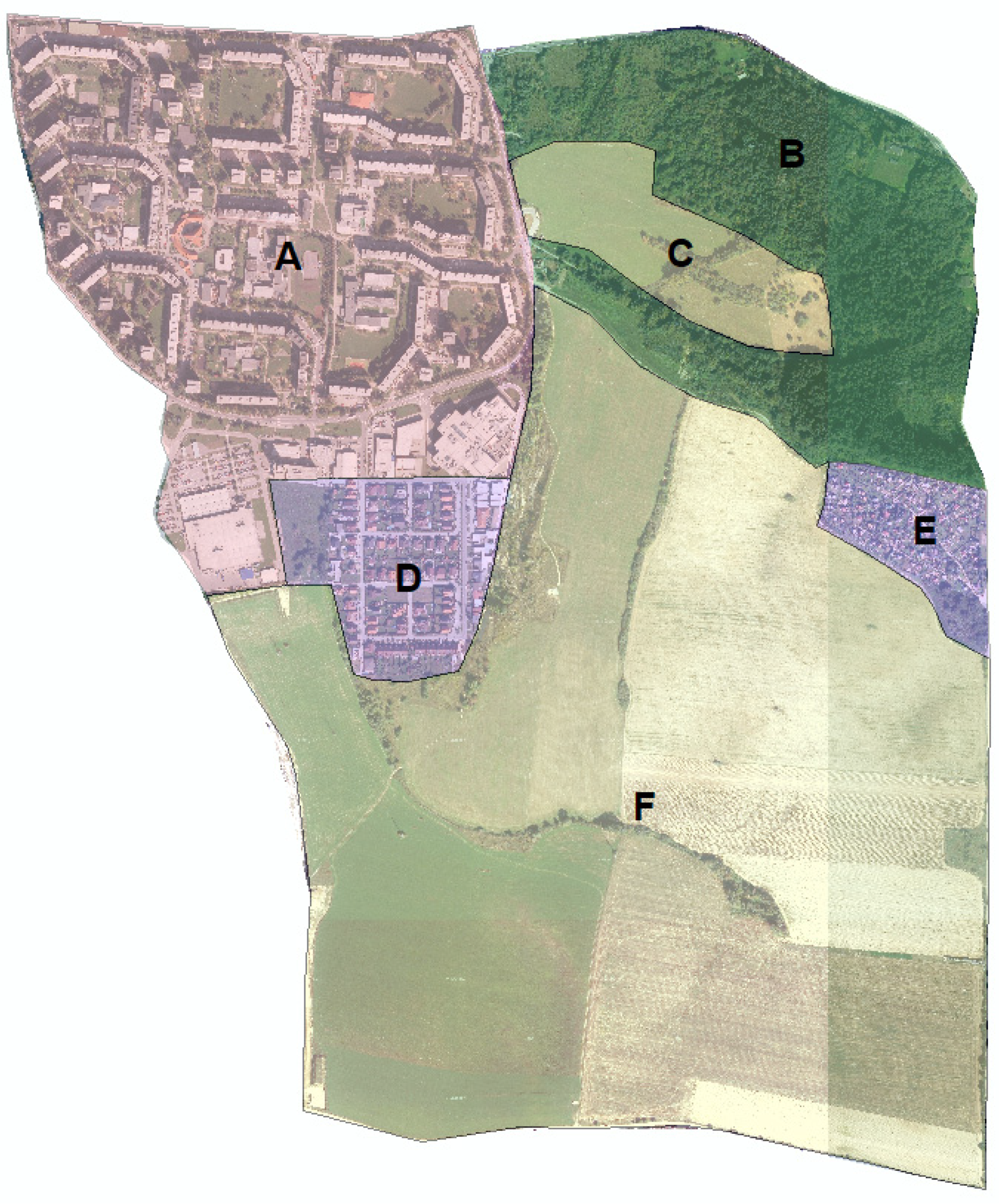
When the locality of interest is about to be chosen, a landscape with wide ranging features would be an appropriate choice [19]. A landscape part spectrum (an open country, forest areas, low built-up areas, habitation) is an ideal choice for the orthophoto-images post processing method for the working environment testing. Accordingly, the wider Solinky surroundings, which form the southern part of Žilina, were chosen. The measured area boundaries were defined as the main settlement catchment area. We may understand the settlement itself and the chosen non-urban part that has been traditionally connected with the settlement, under this term. The settlement extent and dimensions are adequate for the research purposes for the modern data acquisition and postprocessing testing. 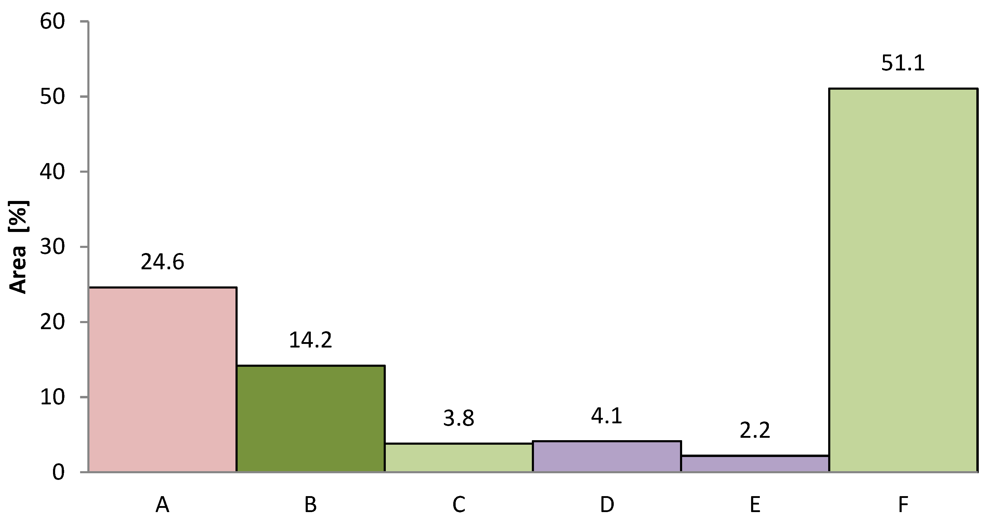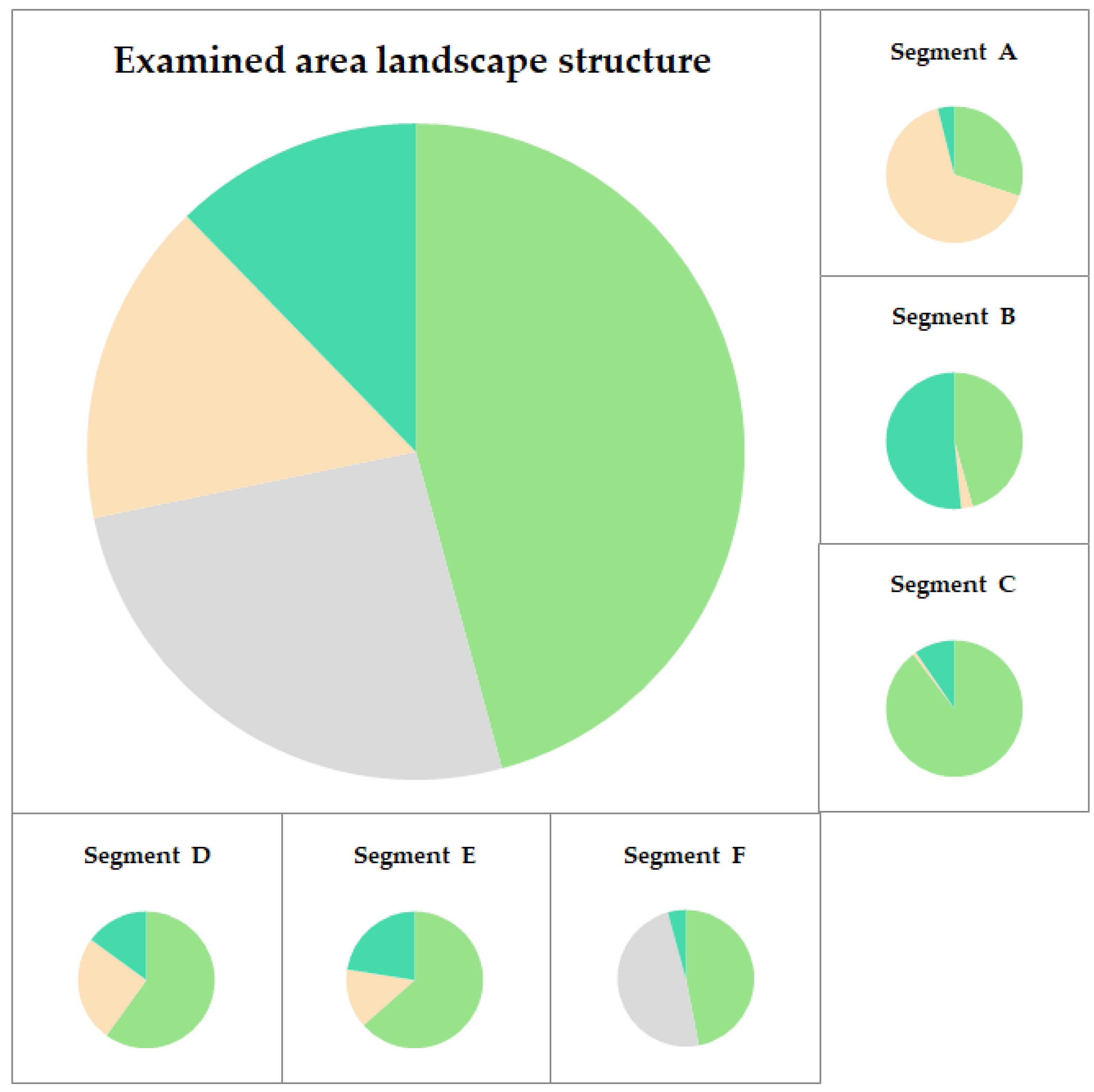In the Figure 1, the basic examined landscape features are depicted based on their use/purpose(s). The examined area includes several landscape features or types, starting with the high built-up areas, segment A (determined by boundaries of the housing estate) represents the settlement itself. The less built-up areas represented by the suburbs, segment D (determined by boundaries of cadastral area), respectively by the gardening areas. Segment E (defined by boundaries of area used for gardening in cadaster of real estates) and various natural feature types used for recreational and agricultural purposes, segments B, C and F (differenced visually for segments B and C and by the boundaries of agricultural usage for segment F). The single segments purpose and percentage are stated in the

Table 7. The examined locality segments types, description and percentage area.

Segment	Land Type	Description	Area (%)
A	settlement, high built-up area	housing and civic amenities	24.6
B	forest park	recreation, microclimate regulation, cultural and ecological purposes	14.2
C	meadows	agricultural utilization, partial recreation purposes	3.8
D	suburbs	low built housing construction, civic amenities	4.1
E	gardening area	recreation, agrotourism	2.2
F	agricultural segment	arable land and permanent grassland for the agricultural purposes	51.1

a graphically depicted in the Figure 2.

The examined locality overall area was 244.2 ha. For the following processing purposes, the correct measuring way and Unmanned Aerial Vehicle (UAV) method is necessary. The measuring method and measured data processing is listed in the following chapter section.

3.2. Aerial Photogrammetry by UAV

In the process of creating a detailed orthographic photograph of the earth’s surface were used only aircrafts. With the current trend of using Unmanned Aerial Vehicles (UAVs) in various applications, unmanned aerial vehicles have found application in this area as well [20]. For the purpose of research and experiment was used UAV DJi Mavic Pro. The experiment consisted of the following phases:

• Definition of the scanned area and orographic situation,
• Definition of way points (Figure 3—left),
• Pre-flight preparation,
• The experiment itself,
• Flight data analysis (Figure 3—right).

The flights were flown in the controlled area of Žilina Airport (LZZI) at a time when the area is in the category ATZ (Aerodrome Traffic Zone) and outside the descent planes GNSS [21], and ILS approach and within the applicable rules of flying and safety procedures [22] with UAV according to Decision no. 2/2019 of 14 November 2019. The front image overlaps of 75% and side overlaps of 65% were used in the imaging, the imaging speed was set to 8 m·s⁻¹. The total flight altitude was 120 m AGL (Above Ground Level) with direct visual contact of the operator. The total flight time was 27 min, during which 2 batteries were used, 487 photos were taken and an area of 115 acres (0.46 square kilometers) was covered.

For images collection was used default camera of DJI Mavic pro drone with following parameters:

• Sensor: 1/2.3” (CMOS), Effective pixels: 12.35 M (Total pixels:12.71 M),
• Lens: FOV 78.8° 26 mm (35 mm format equivalent) f/2.2, distortion < 1.5% Focus from 0.5 m to ∞,
• ISO Range: video: 100–3200, photo: 100–1600,
• Image Size: 4000 × 3000.

The total resolution while maintaining the current flight parameters was 3.3 cm of real distance in the image per pixel. In terms of the selection of the season and time during the day for the implementation of the flight plan [23], the period was selected according to the following parameters. The first most important parameter was imaging with the elimination of shadows [24] from buildings and vegetation. This fact could be avoided by two factors. By choosing a period with the sun as high as possible above the horizon and choosing light meteorological conditions. Aerial photography close to the date of the longest day provided optimal conditions. In terms of meteorological influence, the day was chosen when there were high cirrus cloud conditions in the sky. The cloud type provided lighting conditions and light diffusion that produced softer shadows than on a clear day. In addition to meteorological conditions and forecast [25] for chosen landscape area, the level of developed vegetation in the period without flowers and with leaves was also taken into account. The last factor was the period between precipitation and severe drought. It was the extremes in the supply of water to the ecosystem that caused problems in the subsequent evaluation of the area. One extreme was the formation of soaked soil [26] and the other was the sore dry vegetation. Both cases belong to an environment with vegetation, but by their nature during the evaluation they would be included in an area without vegetation.

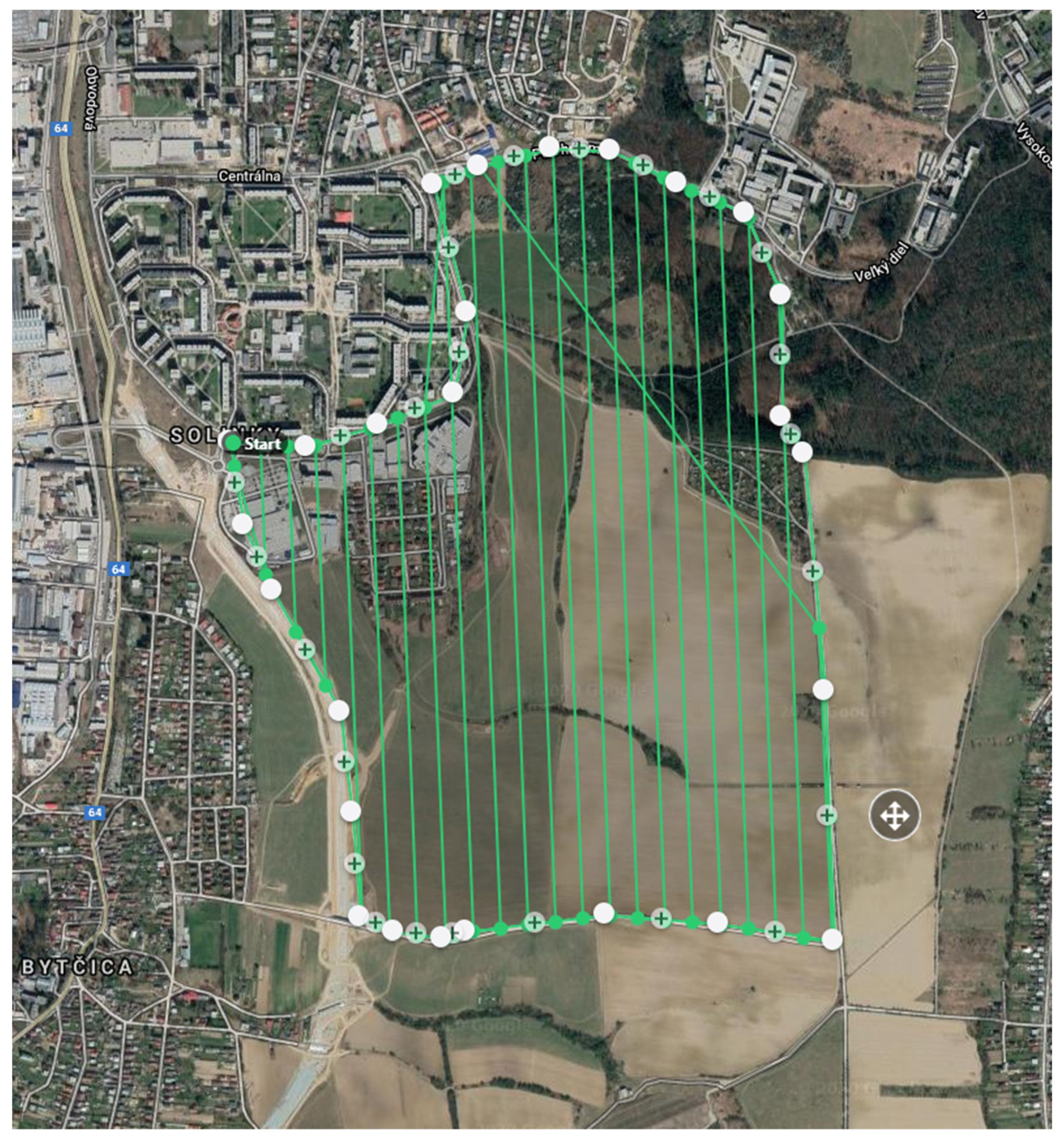
To complete the whole area of research, aerial work has been divided into two polygons. The first polygon was described in Figure 3 and its parameters were defined above. Due to the area of the second polygon (Figure 4), its relief and character, the flight and imaging conditions were adapted to the total flight time. While in the polygon covering the built-up area, the flight altitude was set to 120 m (AGL); when shooting the current polygon, it was 150 m (AGL). Again, all safety conditions were observed during the shooting in accordance with Regulation 2/2019 of the Transport Office of the Slovak Republic in the current conditions of ATZ (Aerodrome Traffic Zone) Žilina. The total aerial photography time of the second polygon was 58 min and a total of 4 batteries were used. The current area was recorded on 1159 images. The resolution of the polygon with the given parameters and a side overlap of 65% and a front overlap of 75% was 2.5 cm per pixel.

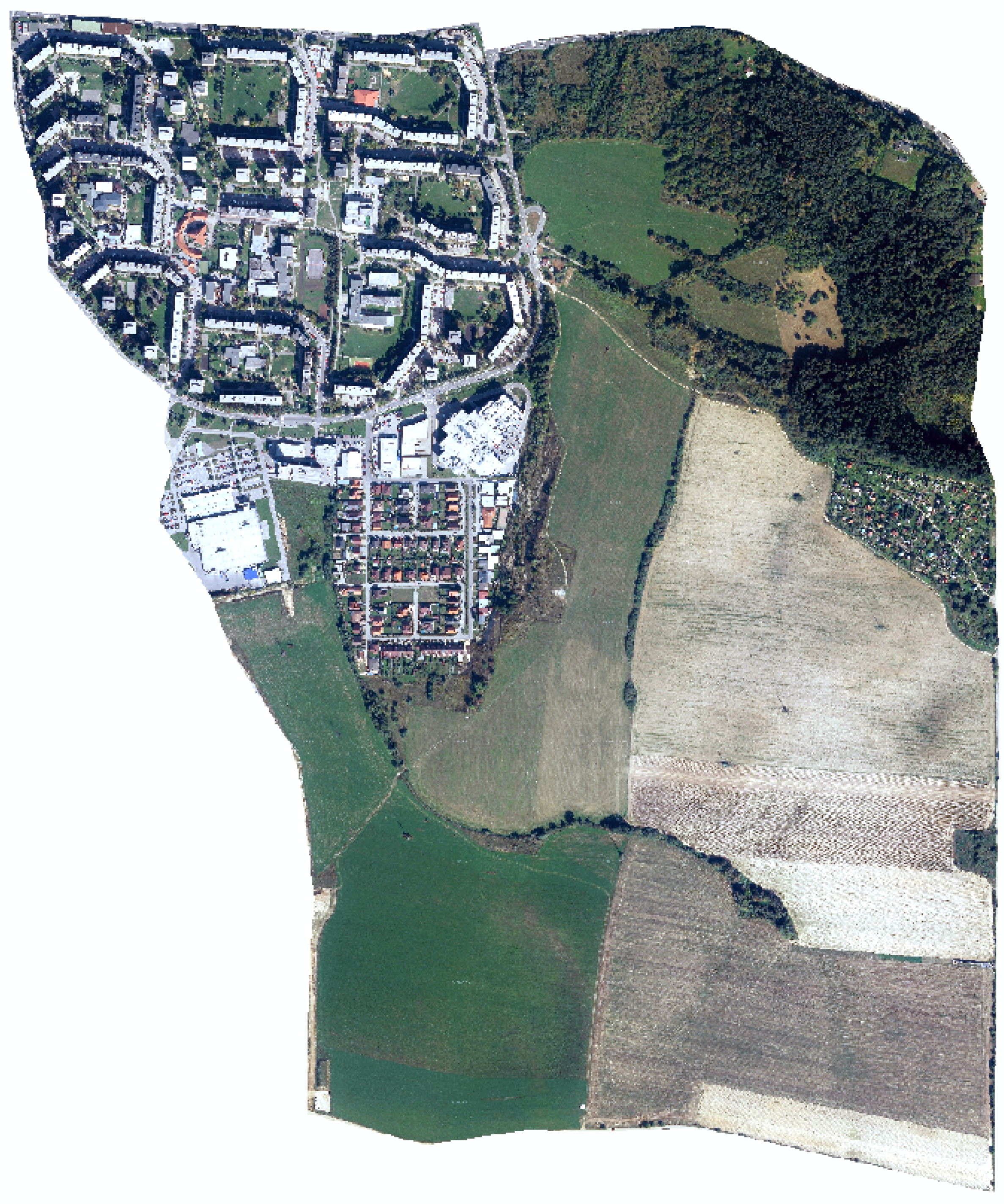
The final clipped area used in the next sections is displayed on the Figure 5.

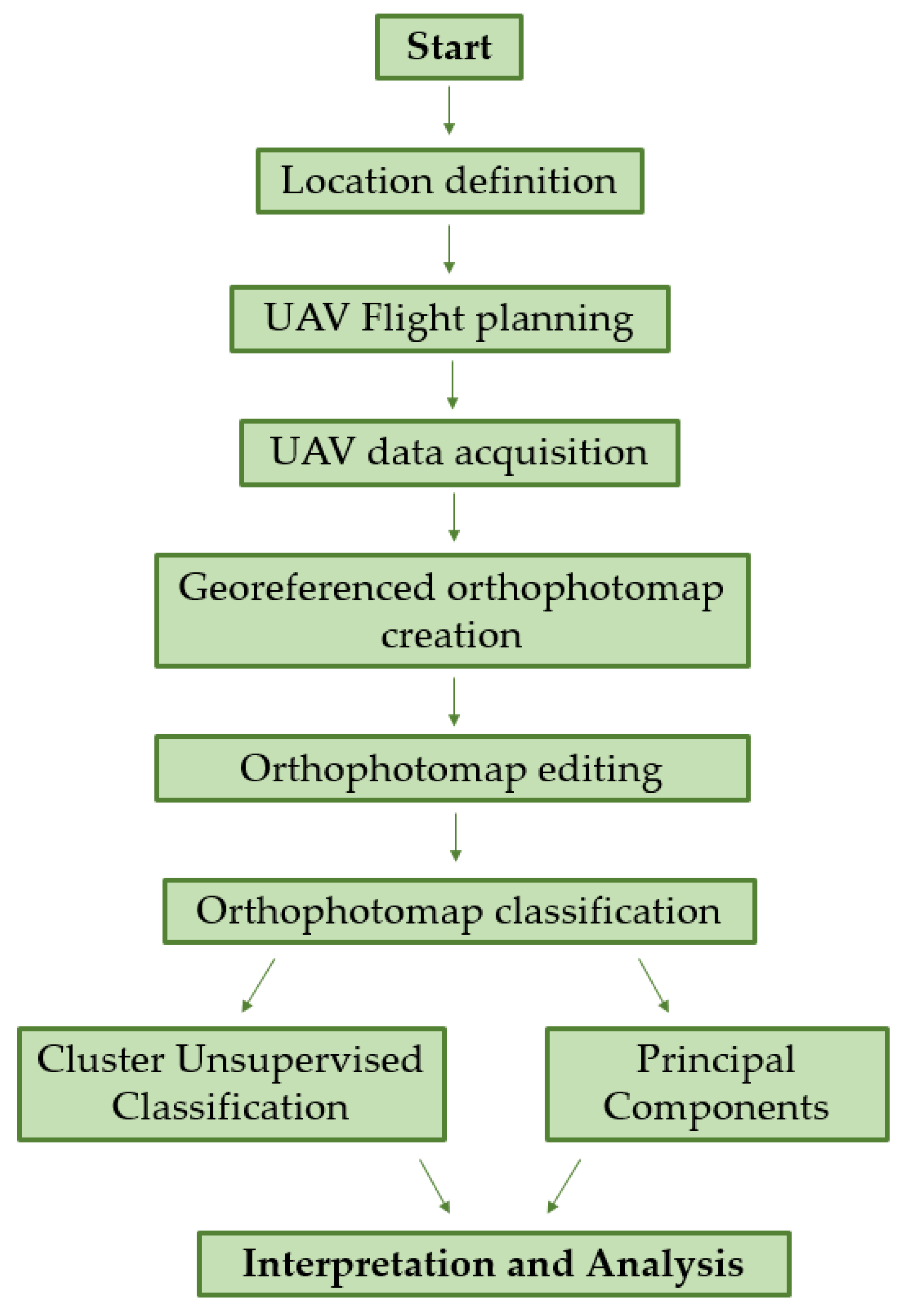
3.3. Postprocessing

The post processing contains various steps. The sample of postprocessing is presented in Figure 6 and it includes steps such as definition of location, which is measured (in our case using the UAV method), the final data must be edited and corrected, for next usage it has to be georeferenced [27,28,29,30]. After the preprocessing, data are able to be used for the aims, that are described below.

After the flight over the area, images processing and orthophoto-images creation, the orthophoto-images were used as the base for the next calculations. Individual orthophoto-images were reclassified in the program ArcMap environment using the toolbar Image Classification, specifically ISO Cluster Unsupervised Classification, as it meets our requirements for the locality of interest orthophoto-images division in the best way. For correct elimination of graphic errors such as shadows, before Cluster Unsupervised Classification, Principal Component was used.

The Principal Components tool is used to transform the data in the input bands from the input multivariate attribute space to a new multivariate attribute space whose axes are rotated with respect to the original space. The axes (attributed) in the new space are uncorrelated. The main reason to transform the data in a principal component analysis is to compress data by eliminating redundancy [16,17,18]. The result of using the tool is a multiband raster with the same number of bands as the specified number of components (one band per axis or component in the new multivariate space). The first principal component will have the greatest variance, the second will show the second most variance not described by the first, and so forth. Principal Components requires the input bands to be identified, the number of principal components into which to transform the data, the name of the statistics output file, and the name of the output raster [19]. The output raster will contain the same number of bands as the specified number of components. The number of components is the same number mentioned earlier. Each band will depict a component [31].

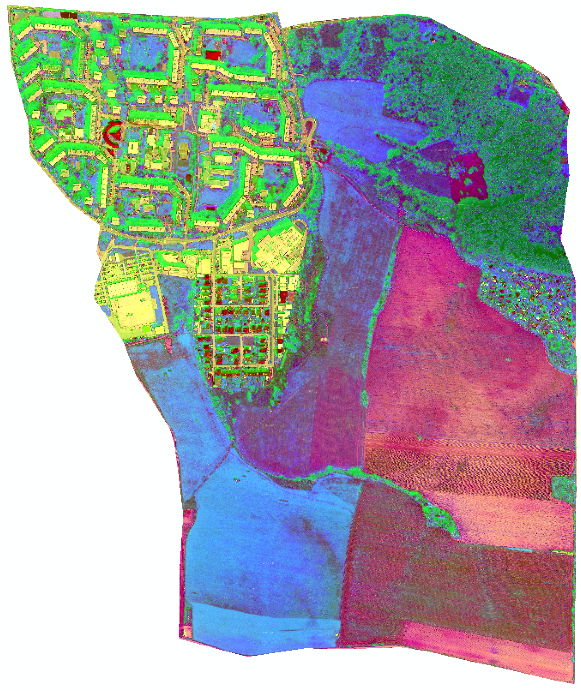
The result of the Principal Components reclassification (post-processing) is displayed in Figure 7. Without any other necessary editing it there is possible to see the differences between basic landscape structures such as built-up areas (mostly in yellow), permanent grasslands (mostly in blue), forest areas (mostly in green) and arable areas (mostly in purple).

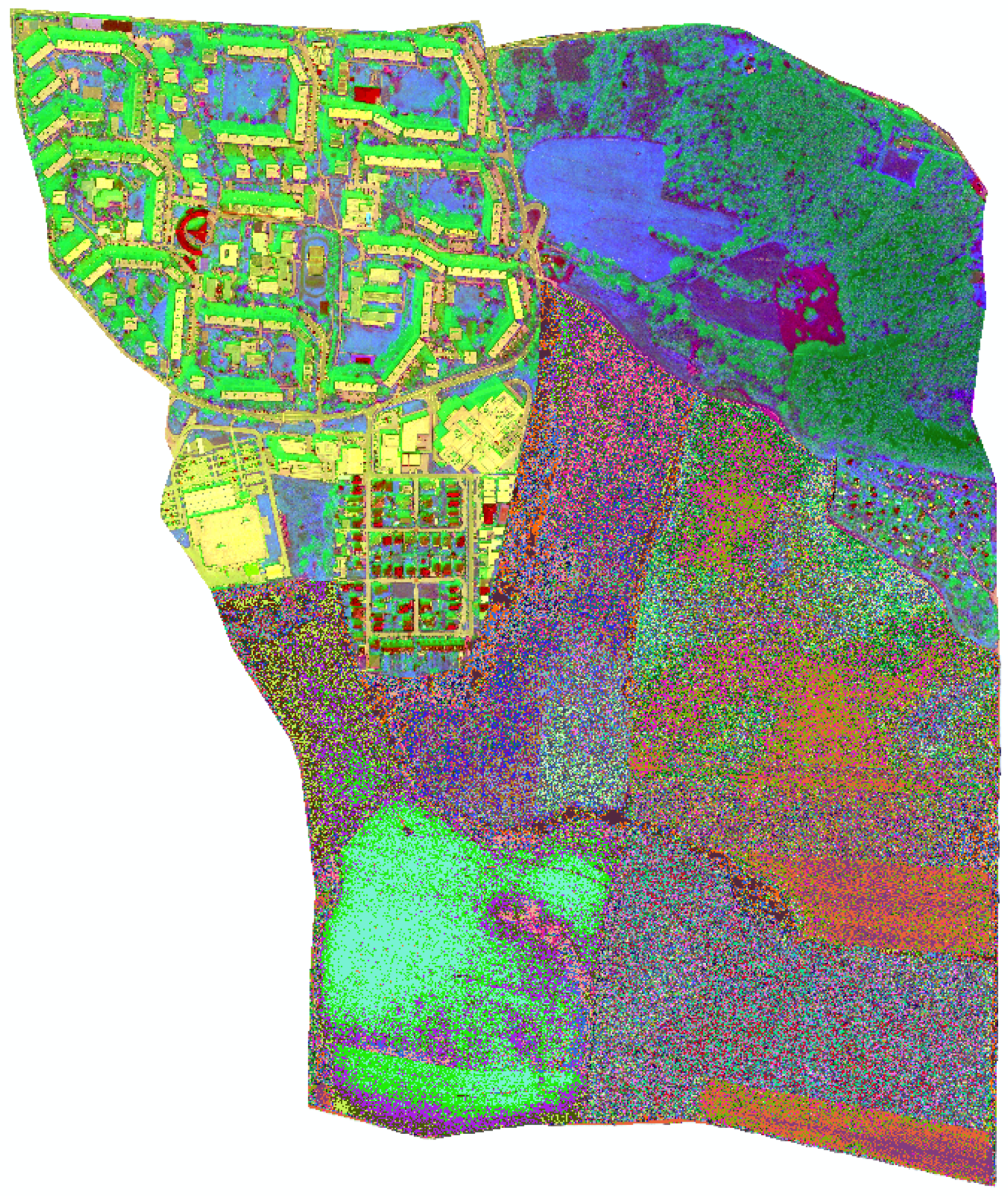
ISO Cluster Unsupervised Classification performs the reclassification of the input orthophoto-image using the Maximum Likelihood Classification tools. This algorithm is based on two principles: The cells in each class sample in the multidimensional space being normally distributed Bayes’ theorem of decision making [20]. To assign each cell to one of the classes the tool takes into consideration both the variances and covariances of the class signatures. If the distribution of a class sample is normal, a class can be characterized by the mean vector and the covariance matrix. These conditions enable determination of the cells membership to the class.

Within the ISO Cluster Unsupervised Classification application in the ArcMap environment [31] after choosing the georeferenced orthophoto-image [32,33], it is necessary to define the number of classes into which the orthophoto-image is about to be classified. The Minimum class size which defines the minimum number of cells in a valid class must be predefined too, together with the Sample interval. This is an interval used for sampling. The number of the intervals within the postprocessing of every single orthophoto-image had to be adopted according to the orthophoto-image content [12]. During the postprocessing the orthophoto-image was divided into the irregular shapes which delimit the landscape structure type. For explanation, in the section formed by the housing development with various roof types, respectively with the various facade color solutions, the misinterpretation may have occurred according to the wrong class determination as it is automatized. If low numbers of classes were used, some valuable structures could fade away in the settlement territory. 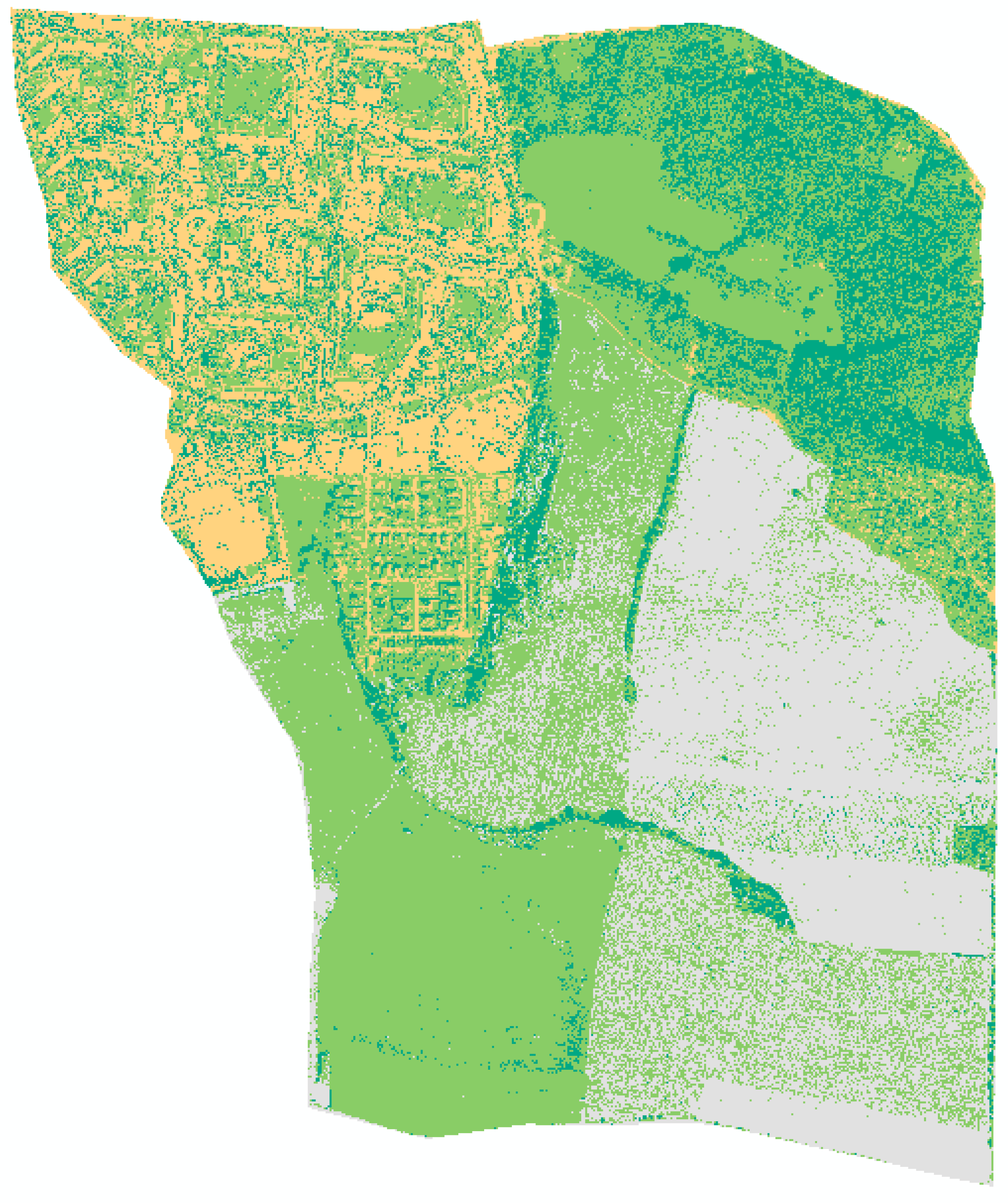In the Figure 8, the reclassified classes of the segment F are possible to be seen. After many experiments the most appropriate number of reclassified classes for built-up areas is 50 and for mostly monocultural areas is 25. The orthopohoto reclassification into four basic landscape structures is displayed in the Figure 9.

According to the reclassification into four basic landscape structures, the area of each land structure was calculated and graphical displayed in the Figure 10. The last step of the post image processing is the calculation of index CES, not only for whole examined area, but also in the separate segments The pixel classification was used due to working with UAV data presented by the orthophoto-image. For the first CES formula, there are no values for the categories, they are only divided into two groups, one is in final calculation the numerator, the other is the denominator, the final CES index presents the ratio of focused area. The index may reach values from 0 up to infinity. For the second CES formula, indexes for single landscape type structures were given as 0.20 for arable areas, 0.50 for temporary grasslands, 0.80 for built-up areas and 1.50 for forest areas. In this calculation, the areas percentage values are necessary. The CES₂ values may reach up to infinity as well. Within the CES₃ calculation, the index for temporary grasslands had to be classified differently for segments A, D, E, where its value was 0.50 which presents garden areas and in segments B, F the index value was 0.62 which presents meadows. The overall CES₃ value of examined locality was calculated as weighted arithmetic mean presented by value 0.59 for temporary grasslands. The index value for built-up areas was given as 0.00. for arable areas 0.14. In the CES₃ calculation, the index value for forest lands was given as 0.63 according to the tree types predominance in the examined areas. Within the CES₄ calculation, the built-up areas are defined as areas with no importance with index 0.00. The index value for arable areas was set as 1.50 that represents the compromise between the areas with low and very low importance. There is not a clearly defined area which can be called a small or large arable land. The index value for meadows is set as 3.00 and for forest areas 4.00 whereas the trees creating forests cannot be defined as natural with index 5.00.

According to the CES calculations using various formulas, single segments reached different CES values, which are object of interpretation. The final CES values are shown in the

Table 8. Final CES values of examined area and single segments.

		Segments
		A	B	C	D	E	F	Whole Examined Area
CES value	CES1	0.51	35.03	121.90	2.98	6.15	1.05	1.38
	CES2	0.40	45.12	90.82	2.60	5.85	3.06	2.30
	CES3	0.18	0.61	0.62	0.39	0.46	0.32	0.35
	CES4	1.06	3.43	3.07	2.39	2.81	2.31	2.25

below.

4. Results Interpretation

The CES₁ points out that segment A, represented by a highly built-up area, is defined as a territory intensively used for mainly large-scale agricultural production [35]; weakened auto-regulatory processes cause a certain ecological lability and all other segments, as well as the whole examined area, can be defined as an almost balanced landscape where the technical objects are relatively in accordance with the preserved natural structures according to Míchal [7]. After the calculation of CES₂, the interpretation is following: segment A is defined as a disturbed landscape, segments D, E, F represent landscapes with dominant natural features, segments B and C may be called natural landscapes, i.e., landscapes close to nature. The whole examined area may be presented as a landscape with dominant natural features. Interpretation based on CES₃ calculation defines segments A and F as unstable landscapes, segments D and E as low stable landscapes and segments B and C as medium stable landscape. The whole examined area is also defined as low stable landscape. Due to CES₄ calculation, segment A is classified as a low ecological stability area with definitions according to Pinto [35], segments D, E, F as medium ecological stability areas and segments B and C as high ecological stability area. The whole examined area is defined as medium ecological stability area.

5. Discussion

According to the above-mentioned calculation results, the CES index calculated based on various author philosophy, segment A represents an area with low ecological stability. In accordance with other authors, the definition is different, but the result is in principle the same. Segment A, separately, may be defined as an unstable area. If the other segments with temporary grasslands and forests in close proximity were not taken into consideration, then segment A would represent an area inappropriate for a high quality and healthy lifestyle, and this fact leads to discussion about the simple land adaptation or another types of landscape remediation. From a wider point of view, the whole examined area is mostly interpreted as a kind of landscape with medium ecological stability index. Segments B and C have the best results and are the reasons the index increases in every CES calculation. CES₃ deserves extra attention, whereas it rates the examined areas in the most critical way. It is the only qualification, that presents segment F as the same unstable area as the high built-up area A. There are also the biggest differences between this type of CES calculation and the others. The question is, which CES calculation is the correct one or captures the ecological stability as realistic as possible?

The aim of this paper was to demonstrate the possible use of UAV’s for CES calculation. This kind of calculation has never been used in this way. CES’s can be calculated from orthophoto-images and this fact makes calculations of CES without terrestrial method possible. This makes the calculations faster and more accessible when there are no terrestrial data sets that can make simple land adaptation less difficult and faster. This may be helpful in the moment of increasing the number of active simple land adaptations.

There are future plans for the study, to apply the possibilities of UAV data usage for CES calculation, due to the different character of wood during the year (such as determination of wood by deciduous trees and evergreen trees or Beeches that are also deciduous, but they only change the color of their leaves). The character of trees has also an impact on CES quality. A future study is going to focus on other areas, not only city areas but villages as well. The results of the research are going to be the basis for simple land adaptations and are also for future ecological and forestry issues.

6. Conclusions

This paper focuses on ecological stability of the landscape. The first part is devoted to legal legislation in this field and points out the different views for various authors to CES calculation. CES indexes presents ecological stability level and various authors show different ways of its calculation and interpretation. The question of correct calculation does not depend only on correct formula but also on the examined area borders and definition. In the case of choosing only strict urban area borders (represented in the paper by segment A), the result would define the examined area as ecological unstable but with different point of view, whereas the wider surroundings are taken into consideration (represented in paper by segments B–F), the results may change and the final CES value would define the examined area as more stable landscape. Additionally, the correct flight may lighten the postprocessing calculations. A flight at the correct time and conditions may avoid many complications. The complications may be represented by presence of shadows, the incorrect vegetation color (deciduous trees without leaves) which is also connected with the seasons, backsides of high buildings, inappropriate daylight during the flight. Another example of weather influence (puddles and mud after long-term rains). The method of using UAV’s in the case of imaging a small area of polygons was much more effective than with the use of civil aircraft. From the point of view of using resources to place the camera in the required flight level and path, this is an incomparably less demanding method. We are talking not only about the financing of aerial work, but also about human resources, fuel and operating costs and, last but not least, the provision of airworthiness management and maintenance [29]. Due to the considerable number of advantages, this study is an advocate of UAV use in specific situations. The use of unmanned aerial vehicles is particularly useful for smaller polygons and in areas where high mapping accuracy is required. In the case of scanning larger areas such as forests or large cities, a method of aerial photography from civil aircraft would be more effective. A number of advantages also include the disadvantages of using unmanned aerial vehicles, such as the risk of loss of signal and thus loss of the entire equipment, collision with ground objects and greater sensitivity to weather conditions. With the growing trend of implementing new technologies, the application of UAVs for the given purposes of orthographic imaging would not have been possible in the past. From the point of view of efficient use of resources, however, the given imaging was suitable and much simpler due to the above-mentioned criteria for the use of unmanned aerial vehicles and civil aircraft.

The correct interpretation does not depend only on precise borders definition but also on the correct CES index calculation formula used. The differences between the calculations according to the various formulas show the disunity of CES index interpretations and should be discussed with specialists from the related fields. The way forward is to choose the proper CES index qualification or to define new ways of CES determination.