New Decentralized Control of Mesh AC Microgrids: Study, Stability, and Robustness Analysis

Abstract

In this paper, we investigated the power sharing issues in mesh islanded microgrids that contain several distributed generators (DGs) and loads connected to different points of common coupling (PCC). Firstly, an improved decentralized droop control algorithm is proposed to achieve the active and reactive power sharing of different DGs in reconfigurable mesh islanded microgrids. Accurate power sharing was obtained even though line parameters or the mesh microgrid configuration were unknown. Secondly a state-space model of the whole mesh microgrid was developed, considering several generators with their decentralized controllers, line feeders, and dynamic loads. This model was used to design parameters of droop controllers, to study the asymptotic stability and the robustness properties of the system. All strategies and analyses were validated by simulation based on the generic microgrid detailed in the standard IEEE 9bus test feeder.

1. Introduction

Microgrids are able to integrate different distributed generator (DG) systems converting different types of renewable energy and to supply different types of loads. This gives a certain level of independence, allowing them to be connected or disconnected from the main grid. One of the challenges is to synchronize and connect all the distributed generators to an islanded microgrid, while providing the “plug and play” functionality and respecting the active and reactive power sharing between the different distributed generation units (DGs) [1,2]. Currently, the most used methods for power sharing and synchronization in literature are based on the droop control strategy [3,4,5,6,7,8]. However, most of the microgrids considered in these research works have only a single point of common coupling (PCC), which are connected to all DGs through converters and the loads like in Figure 1. In order to level up the independence of microgrids from the main grid by increasing the penetration rate of distributed generators in microgrids, the choice of mesh multi-PCC microgrids seems to be a good solution. However, the intermittency of renewable energy may cause more instability problems in mesh microgrids due to their higher level of complexity compared to microgrids with single points of common coupling.

In mesh multi-PCC reconfigurable microgrids, with many distributed generation sources (DGs) and loads randomly connected to different PCCs, classical synchronization methods and power sharing strategies based on droop control and used in mono-PCC microgrids are less efficient. Indeed, most droop methods assume that the transmission lines are purely inductive or resistive in nature which leads to a linear droop characteristic where active power sharing depends on either frequency or voltage magnitude. However, in microgrids with reconfigurable structure, the sources as well as the networks may become redundant. The changes in the network impedance whenever a branch or source is disconnected in a microgrid means that the active and reactive power cannot be totally decoupled. These changes affect the power sharing among the sources and reduce the stability of the microgrid for any disturbance [9,10].

Much research has focused on solutions that concern the active and reactive power sharing in droop-controlled mesh microgrids [11,12] either by using virtual impedance correction loop and a convergence acceleration strategy to compensate the offset created by the power line impedances and improve the reactive power sharing such as in ref [11], or by adopting a voltage compensation strategy to keep the bus voltage stable at the rated value and improve the reactive power sharing such as in ref [12]. However, only a few studies have focused on active and reactive power sharing in reconfigurable mesh microgrids such as in ref [10], where the authors propose the use of L1 adaptive methods for stable operation of a microgrid with wide range of R/X ratios.

Another problem is the possible unstable behavior of the microgrid caused by the interaction between the DGs and loads as well as the changes in the network configuration. The system stability depends on the type of loads being connected to the microgrid, especially the ones supplied through tightly regulated power converters. These loads behave as constant power loads (CPL) and may cause system instability [13,14,15]. In the literature, the main studies are based on linearization techniques [16]. The non-linear models of the considered power systems are linearized around an operating point and then studied using linear analysis tools. Moreover, linearization tools only predict the stability of the system for small perturbations [17,18] and cannot guarantee the system stability for large perturbations.

In this paper, a mesh microgrid constituting several PCCs connected to two DGs (DG1 with a nominal power of three megawatts and DG2 with a nominal power of two megawatts) through two transformers (6 kV/20 kV) as well as three loads (LOAD1 with a nominal power of one megawatt, LOAD2 with a nominal power of 1.2 megawatts, and LOAD3 with a nominal power of 1.5 megawatts) are considered. The different PCCs are interconnected with power supply lines, modeled by resistance, inductance and capacitance (RLC) circuits inspired by an IEEE 9-bus test feeder (Figure 2). All the microgrid data are presented in

Table 1. Parameters of the considered microgrid power lines.

Lines	Resistance (Ω)	Inductance (mH)	Capacitance (µF)	Points of Connections
Line 1	0.63	7.14	205	Bus 8–Bus 7
Line 2	2.55	11.4	230	Bus 5–Bus 7
Line 3	0.63	7.14	205	Bus 8–Bus 9
Line 4	2	7	180	Bus 9–Bus 6
Line 5	1.7	7.6	153.4	Bus 4–Bus 5
Line 6	1.7	7.6	153.4	Bus 4–Bus 6

and

Table 2. Sources and load powers.

Sources and Loads	Active Power (Mw)	Reactive Power (Mvar)	Phase to Phase Voltage (kV)	Point of Connection
Source 1	3	0.9	6	Bus 7
Source 2	2	0.9	6	Bus 9
Load 1	1.5	0.35	20	Bus 5
Load 2	1.2	0.25	20	Bus 6
Load 3	1	0.25	20	Bus 8

.

In order to ensure an accurate power sharing and to provide the “plug and play” function adapted to the considered multi-PCC mesh microgrid, a new droop control and synchronization strategies is applied, such as the one demonstrated in ref [19]. This new droop control in islanded mode consists of removing the decoupling between the active and reactive power caused by the line impedances and the change in the microgrid configuration. The first DG connected to the microgrid imposes its voltage and frequency. For other DGs, an adapted synchronization strategy is proposed and applied before their interconnection to the microgrid. The simulation results using a model developed in the Simscape feature of MATLAB/Simulink environment enabled the validation of the efficiency of this new droop control.

To study the stability of the microgrid, a state model of the entire meshed micro-grid was developed considering its power lines and loads including a CPL as well as its generators, with their decentralized controllers integrating modified droop algorithms. The comparison of the results obtained from the stablished state model and the developed model in Simscape environment confirm the validity of the proposed microgrid state model. This validated state model was then used to study the microgrid stability by calculating its Jacobean matrix and its eigenvalues at each operating point. Based on these results, the root locus, and eigenvalues sensitivity analysis, depending on the parameters of the established model, were performed. The latter made it possible to find the origin of different frequency components by observing the dynamic behavior of different state variables. The analysis of the system stability was then performed by observing the evolution of the system eigenvalues with respect to droop parameters and different load power variations. It will be shown that the system stability may be affected due to unadapted droop control parameters and/or CPL levels.

The established state-model was also used to verify the robustness of the considered mesh microgrid, including the new droop-control that ensured active and reactive power sharing to the modifications caused by the connection of DGs and large load variations (changes in network configuration).

To summarize, the main points of this paper are, firstly, the development of a new droop control strategy for power sharing especially reactive power in mesh islanded microgrids. Unlike in the solutions mostly used by authors for power sharing in reconfigurable mesh microgrids, this modified droop control strategy is decentralized, which means that it does not require any sort of communication between the DGs connected to the microgrids. Thanks to the non-linear term added to the classical droop control, the power coupling phenomenon created by the line impedances and the change in the microgrid configuration is removed. The modified droop control strategy was proven efficient for active and reactive power sharing in different microgrid structures. Additionally, a fast and efficient synchronization strategy did not affect the power sharing. The second major point is the development and validation of a state-space model describing the mesh microgrid and its control. This state-space model was used to study the microgrid stability especially in the presence of active loads such as CPLs. The state model was also used to test the robustness of the modified droop control under different microgrid configurations and different states of charge. The validated state-space model made the manipulation of the system so much easier and allowed many more studies to be carried out on the meshed microgrid. For example, one of many scenarios where the state-space model can be useful is when the CPL-injected power in the microgrid increases, and the state model can easily predict the right value of the capacitor that should be added to the PCC where the CPL is also connected. This means that many future studies can be conducted based on this developed and validated state-space model.

2. Power Sharing and Synchronization Strategies in Mesh Microgrids

2.1. Power Sharing Using Droop Control Strategies

The traditional droop strategy imposing the electrical pulsation and the RMS voltage of a distributed generator via Equations (1) and (2) is efficient in microgrids with a single PCC shown in Figure 1, only if the effect of power line impedance is ignored [4].

$${\omega }_i= {\omega }_n- m_i\left(P_i-P_{in}\right),$$

(1)

$$E_i= E_n- n_i\left(Q_i-Q_{in}\right)$$

(2)

$$\mathrm{With}:{ m}_i= \frac{{\Delta }_{\omega }}{P_{in}},{ n}_i=\frac{{\Delta }_E}{Q_{in}},$$

where $P_i$ and $Q_i$ are the measured values of the active and reactive power of the ith DG,$P_{in}$ and $Q_{in}$ are their nominal values, ${\omega }_n$ and $E_n$ are the nominal values of the pulsation and voltage of the ith DG, ${\Delta }_{\omega }$ and ${\Delta }_E$ are the permissible variations of pulsation and voltage, and $m_i$ and $n_i$ are the droop control coefficients. The active and reactive power sharing method is based on a droop control algorithm that sets the frequency and voltage amplitude at the associated PCC for each DG according to Equations (1) and (2).

This droop control does not ensure efficient reactive power sharing even in single PCC micro-grids due to the line impedances. A droop control strategy that has been proven effective for active and reactive power sharing in mono-PCC microgrids (3) and (4) was applied to the complex mesh microgrid in Figure 2, and considering one of the PCC voltages as reference potential of the studied microgrid. The simulation results are presented in Figure 3 and Figure 4.

$${\delta }_i=\int \left(K_a\left({\delta }_{\mathit{in}}-{\delta }_L\right)-m_i\left(P_i-P_{\mathit{in}}\right)\right).dt,$$

(3)

$$E_i=\int \left(K_e\left(E_{\mathit{in}}-E_L\right)-n_i\left(Q_i-Q_{\mathit{in}}\right)\right).dt,$$

(4)

The proposed angular droop aims to indirectly control the voltage at the PCC and its phase to be equal to the nominal values (i.e., $E_{\mathit{in}}$ and ${\delta }_{\mathit{in}}$). The added integrators can minimize the static error between the feedback signal and the corresponding nominal values. By choosing identical $K_a$ and $K_e$ for each generator, an accurate active and reactive power sharing is achieved which no longer depends on the system impedance and is unaffected by the digital errors and disturbances [9].

In practice, real microgrids can have several PCCs, interconnected by several supply lines with non-negligible impedances. In order to study such a microgrid, a slightly modified IEEE 9bus test feeder is considered, composed of two DGs and three loads, interconnected by RLC lines (Figure 2). It can be noticed that the application of the droop method, based on Equations (3) and (4), on the multi-PCC microgrid of Figure 2 leads to a perfect active power sharing when the second DG is connected at 5 s (Figure 3a). However, the reactive power sharing when the second DG is connected is not achieved (Figure 3b). It can also be remarked that unacceptable disturbing active and reactive power peaks occur due to the lack of synchronization (Figure 3a,b at 5 s).

In mesh microgrids, each line, connecting the ith PCC to the jth, has a non-negligible inductance (${\lambda }_{i,j}$) and resistance (${\rho }_{i,j}$), leading to a line voltage drop between these two PCCs that creates a coupling between the active power ($P_{i,j}$) and reactive power ($Q_{i,j}$) exchanged between ith and jth PCCs, according to Equation (5):

$$\Delta E={\rho }_{i,j}{I}_{i,j}cos\phi +j{\lambda }_{i,j}\omega I_{i,j}\sin \phi =\frac{{\rho }_{i,j}{P}_{i,j}+j{\lambda }_{i,j}{Q}_{i,j}}{E_i},$$

(5)

where φ is the phase shift between the phase voltage ${\overline{E}}_j$ and the phase current $\overline{I_{i,j}}$.

To achieve an efficient reactive power sharing in this type of mesh microgrids, the voltage equation in (2) is modified by adding a decoupling term (see Equation (7)) removing the coupling phenomenon between active and reactive power [12]. This coefficient, called $J_i$, is estimated using a PI controller, forcing the suppression of the error ${\epsilon }_i$ defined in Equation (8). In steady state, when the error ${\epsilon }_i$ tends to zero, the reactive power sharing is well ensured between the DGs. This approach allows the primary control of the voltage of the ith DG, regardless of the operating point of the loads. It should be noted that $E_{ref}$ in Equation (8) is the measured value of one of the PCC voltages of the studied mesh microgrid acting as the pilot node and considered as its reference potential. The rated voltage of this pilot node is called $E_n$.

$${\omega }_i={ \omega }_n-{ m}_i\left(P_{fi}-P_{in}\right),$$

(6)

$$E_i= E_n-{ n}_i\left(Q_{fi}-Q_{in}\right)-J_i\left(P_{fi}-P_{in}\right),$$

(7)

$$\mathrm{With}: m_i= \frac{{\Delta }_{\omega }}{P_{in}},{ n}_i=\frac{{\Delta }_E}{Q_{in}} \mathrm{and} \{\begin{array}{c}{J}_i=K_I\int {\epsilon }_{i}dt\\ {\epsilon }_i=\left[-\left(\frac{E_{ref}}{E_n}-1\right)-\left(\frac{Q_i}{Q_{in}}-1\right)\right]\end{array},$$

(8)

In the absence of information on $E_{ref}$ the coefficient J is set to 0 and we return to the classical droop.

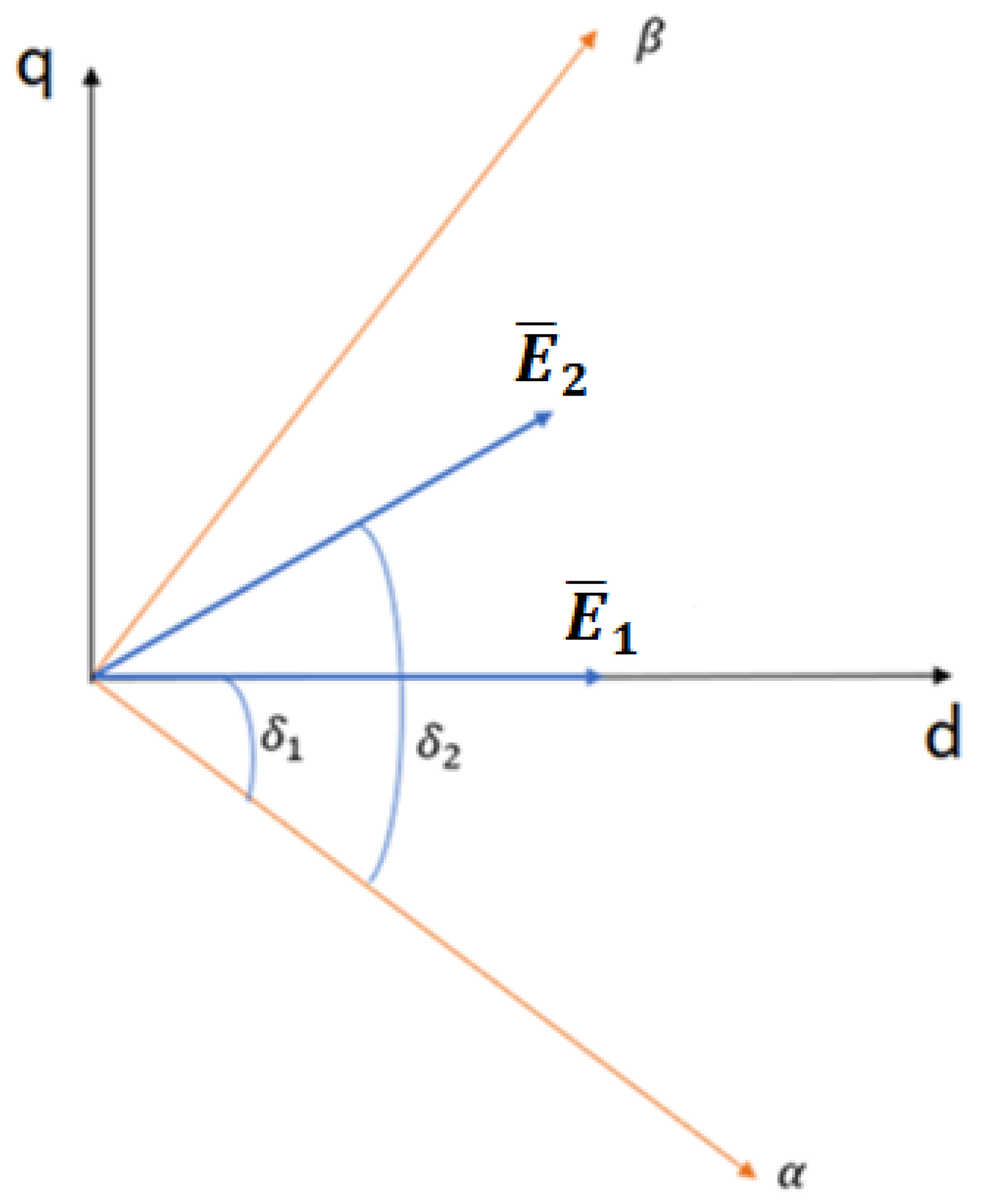
2.2. Synchronization Strategy in Mesh Islanded Microgrid

Due to the complexity of the mesh microgrids and the intermittency of renewable energies, DGs frequently connect to and disconnect from the microgrid, so a fast and efficient synchronization method is required. To achieve the synchronization of the ith DG to the ith PCC before their interconnection, the voltage amplitude $E_{pcci}$, the pulsation ${\omega }_{pcci}$ and the phase ${\mathsf{\theta }}_{pcci}$ of the ith PCC must be approximately equal to those of the ith DG $\left(E_{DGi},{\omega }_{DGi},{\mathsf{\theta }}_{DGi}\right)$ [2]. To achieve this objective, the errors between the amplitudes, pulsations, and phases of both sides (the ith DG and the ith PCC) are forced to zero by adding pure integral controllers to the ith DG droop control, as shown in Equations (9) and (10) [19]. It should be noted that the binary coefficient $B_i$ in these equations is equal to one only during the synchronization interval, and equal to zero otherwise. For the pulsation and phase synchronization, the pure integrators are added to the pulsation droop control, Equation (9), and for the voltage synchronization, the pure integrator is added to the voltage droop control, Equation (10).

$${\omega }_i={ \omega }_n-{ m}_i\left(P_{fi}-P_{in}\right)-\left[K_{ai}\int \left({\omega }_{DGi}-{\omega }_{pcci} \right)+K_{bi}\int \left({\mathsf{\theta }}_{DGi}-{\mathsf{\theta }}_{pcci}\right)\right]B_i,$$

(9)

$$E_i= E_n-{ n}_i\left(Q_{fi}-Q_{in}\right)-J_i\left(P_{fi}-P_{in}\right)-\left[K_{ei}\int \left(E_{DGi}- E_{pcci}\right)\right]B_i,$$

(10)

To prove the efficiency of the proposed synchronization and power sharing strategies, the mesh microgrid in Figure 2 is modeled using the Simscape toolbox of Matlab/Simulink. Source 1 and Source 2 of Figure 2 are modeled by two controllable voltage sources shown in Figure 4, connected to two different PCCs and controlled by $E_{ab{c}_{refi}}$, which was generated using the modified droop strategy described by Equations (9) and (10), a power calculation bloc, a power filter, park transform and inverse park transform, as explained in the equivalent synoptic diagram describing a droop-controlled DGi in Figure 5. The main microgrid parameters are listed in Table 1. The powers of sources and loads are listed in Table 2.

Based on this Simscape model, the efficiency of the proposed synchronization and power sharing strategies assumed in Equations (9) and (10) is evaluated. Figure 6a and 6b show the evolution of the active and reactive powers delivered by DG1 and DG2. In the beginning, the first DG (DG1) imposes the frequency of the microgrid as well as the voltages of each PCC; up to t = 5 s, DG1 supplies the loads connected to the microgrid. The second generator (DG2) is synchronized during the interval 1–5, and then it is connected to the microgrid at t = 5 s. The power-sharing of the active and reactive powers are ensured in steady state without being affected by the synchronization procedure. In addition, compared to the previous results shown in Figure 3a,b, the power peaks appearing after the connection of DG2 to the microgrid are considerably attenuated. It should be noted that these performances are maintained with a higher number of DGs connected to the microgrid, even though the results are not presented in this paper.

In order to highlight the effect of the loss of the information on $E_{ref}$, a simulation test was made using the developed model in Simscape environment, and the results are shown in Figure 5. It consists of connecting both DGs to the microgrid at 0 s using the control strategy defined in Equations (6) and (7). The information on $E_{ref}$ is lost at 4 s and becomes available again at 8 s, and in this scenario Figure 7a,b show the evolution of the active and reactive powers, respectively. The active power sharing is not affected by the loss of information on $E_{\mathrm{ref}}$ because it only depends on the frequency, being the same in all the microgrid PCCs. However, the reactive power sharing is totally lost when the information on $E_{\mathrm{ref}}$ is absent, but it is easily regained when the information on $E_{\mathrm{ref}}$ becomes available again.

Even though the considered microgrid including its loads and DGs are well controlled, the synthesis of the droop control parameters is not based on a methodical approach; they are tuned by trial-and-error method using Simscape.

This method cannot guarantee the system stability when the parameters of the load change or additional dynamical constant power loads (CPL) are connected to the microgrid. For example, when a CPL is added to the microgrid it is not evident to foresee the system stability with the variation of its absorbed active power. Figure 8 shows that, as previously, the first DG1 imposes the frequency of the microgrid as well as each PCC voltage of up to t = 5s and supplies the R–L loads connected to the microgrid. The second generator (DG2) is synchronized and connected to the microgrid at t = 5 s. A dynamic CPL is connected parallel to load 1 (see Figure 2) at t = 7 s, absorbing an active power of 120 kW and zero reactive power. The active power absorbed by this CPL is increased to 500 kW at t = 8 s. It can be remarked that the connection of the CPL absorbing 120 kW does not impact the stability, but when its absorbed power increases to 500 kW the system becomes unstable. Hence, for each modification, the trial-and-error method should be applied again in order to find the eventual new values of the microgrid control parameters which may ensure its stability. In order to overcome this constraint, one solution consists of establishing the state-model that represents the microgrid including its control and studying the microgrid stability by calculating its Jacobean matrix and its eigenvalues at each operating point, as is detailed in the next section.

3. System Modeling for Its Stability Analysis

Due to the interaction between the DGs and the loads, the stability of the microgrids is strongly influenced. Therefore, to study the stability and robustness of the droop-controlled microgrid, a complete mathematical dynamic model of the whole system is established in this section.

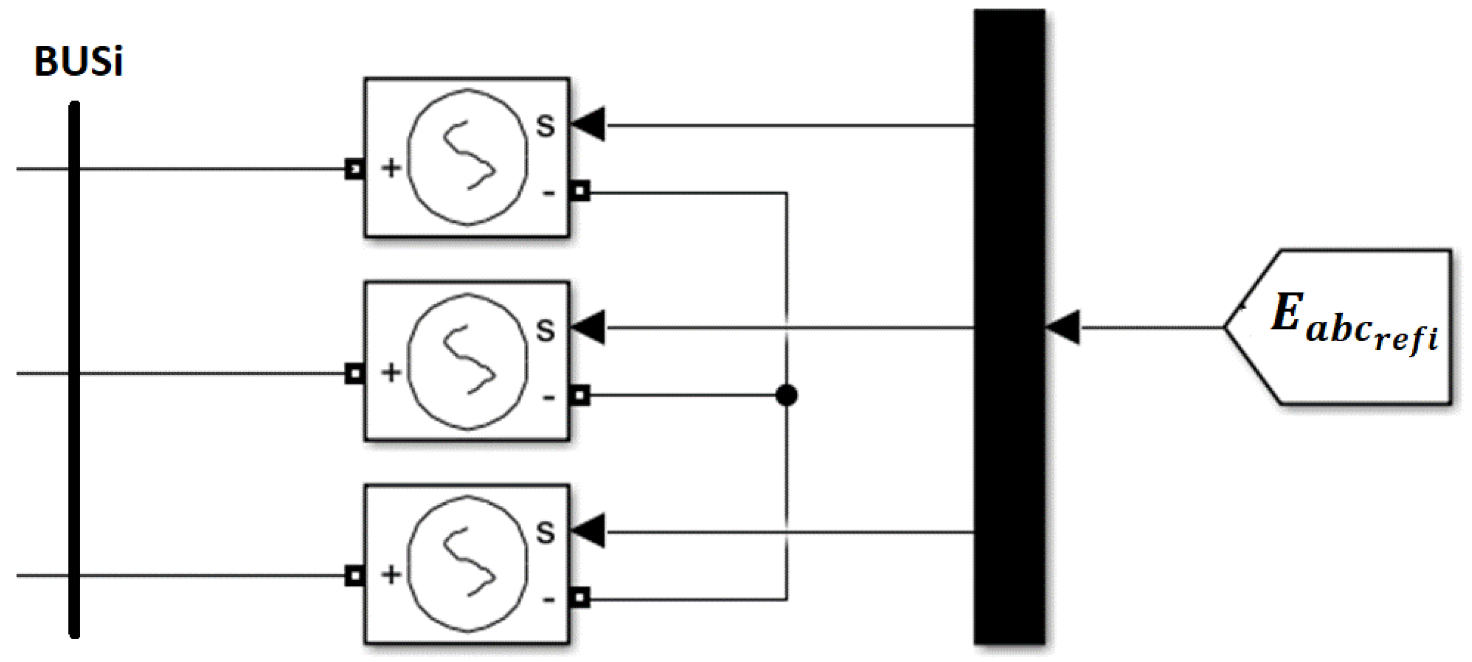
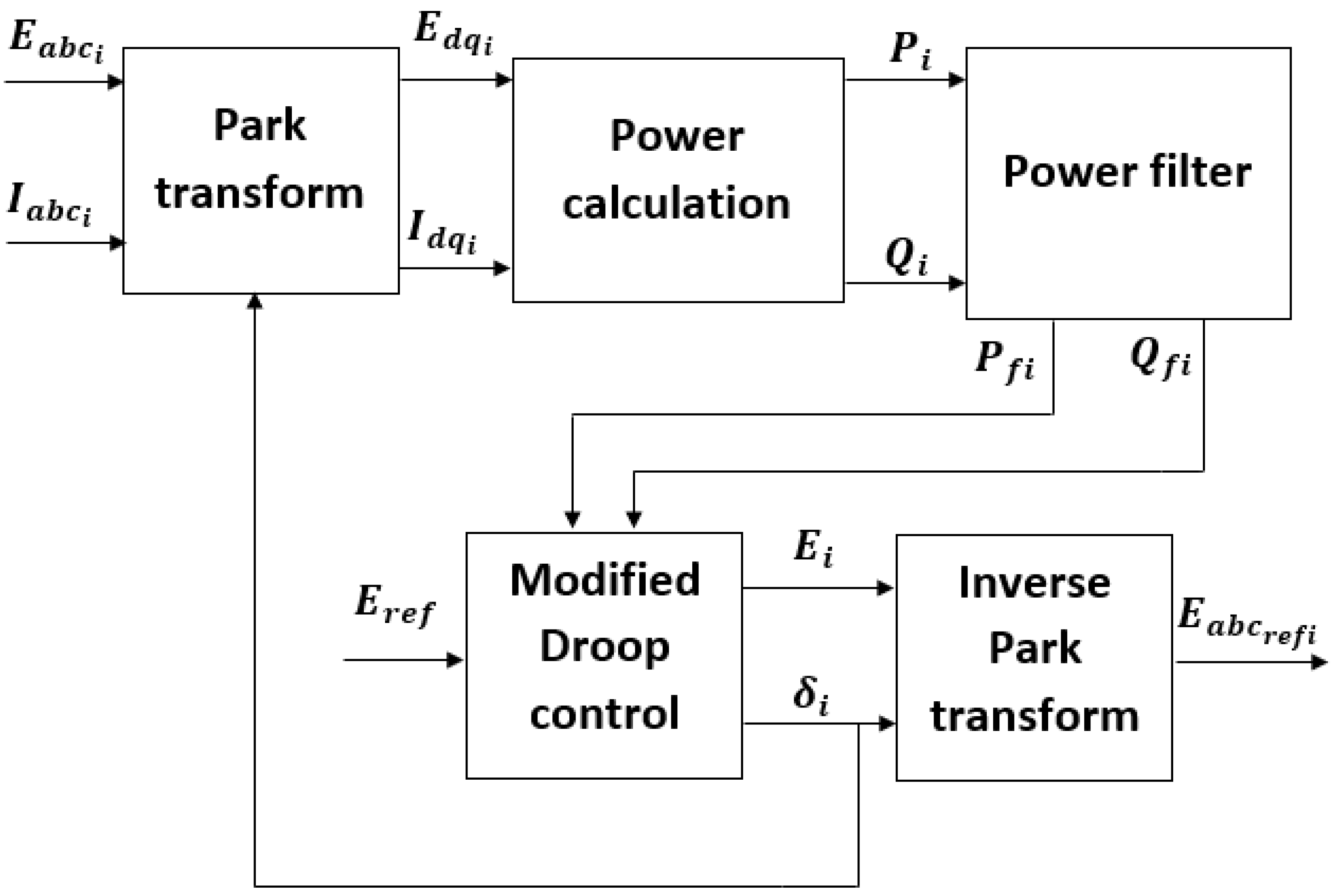
3.1. State-Space Model of a Distributed Generator (DG)

The equations describing the behavior of the ith DG are presented on the equivalent synoptic diagram of Figure 9. It is composed of four cascaded blocs for which the relationship between their outputs and inputs are presented in the following.

In the first bloc (Figure 9), the ith DG measured voltages ($E_{i_d}$, $E_{i_q}$) and currents ($i_{di}$, $i_{qi}$) are used to calculate the instantaneous active and reactive powers using classical Equations (11) and (12).

$$P_i=E_{i_d} . i_{i_d}+E_{i_q} . i_{i_q}$$

(11)

$$Q_i=E_{i_q} .i_{i_d}-E_{i_d} . i_{i_q}$$

(12)

In the second bloc, the instantaneous active and reactive powers ($P_i$ and $Q_i$) are filtered using a first-order low-pass filter to obtain the average (filtered) values $P_{fi}$ and $Q_{fi}$ using Equations (13) and (14). It should be emphasized that the cut-off frequency ${\omega }_f$ of the filter is related to the dynamics of the droop control-loop.

$$\frac{d}{dt}{P}_{fi}={\omega }_f\left(P_i-P_{fi}\right)={\omega }_f\left(P_i-P_{fi}\right)$$

(13)

$$\frac{d}{dt}{Q}_{fi}={\omega }_f\left(Q_i-Q_{fi}\right)={\omega }_f\left(Q_i-Q_{fi}\right)$$

(14)

The third bloc applies the modified droop control in Equations (6)–(8), using $P_{fi}$ and $Q_{fi}$ to achieve the active and reactive power sharing.

The fourth bloc models the delay imposed by the voltage source inverter (VSI), controlling the ith DG output voltages by means of a second-order filter. This filter has a faster dynamic compared to the external droop control loop ${\omega }_c\gg {\omega }_f$. The relationship between the output voltage of the ith DG and its voltage reference is expressed by the transfer function defined in Equation (15):

$$\frac{E_{i_{dq}}}{E^{\ast }{}_{i_{dq}}}=\frac{{\omega }_c{}^2}{s^2+2\xi {\omega }_c.s+{\omega }_c{}^2},$$

(15)

3.2. Microgrid Structure and Modeling

Figure 10 shows a microgrid inspired from the IEEE 9bus test feeder that differs slightly from the microgrid of Figure 2 and contains an additional CPL. In fact, this type of load is increasingly present in microgrids and imposes more severe constraints to the system stability. The considered microgrid is composed of two DGs powering three classical inductive loads, modeled by serial R–L circuits, and a CPL load. They are interconnected by RLC power lines to represent a mesh multi-PCC microgrid. The line connecting the $PC{C}_i$ and $PC{C}_j$ have a resistance $r_{ij}$, an inductance $l_{ij}$, and a capacitance of $c_{ij}$. Their values are determined knowing the distance between the considered PCCs. The capacitance $c_{ij}$ is connected to the $PC{C}_j$.

In order to study the considered microgrid having two DGs, the state equations are given using a common reference frame for expressing the different variables. The used d–q reference frame is defined in a way that its d-axis is oriented toward the first DG voltage vector (${\overline{E}}_1$ Figure 11). Then, the d-axis is shifted by ${\delta }_1$ with respect to the $\alpha$-axis, where ${\delta }_1$ is the argument of the DG1 voltage vector (${\overline{E}}_1=E_1{e}^{j{\delta }_1}=E_{1_{\alpha }}+j{E}_{1_{\beta }}$). The rotating d–q reference frame turns with an electrical speed of ${\omega }_1=\frac{d{\delta }_1}{dt}$ with respect to the fixed reference frame $\alpha -\beta$. When the different DGs are synchronized and connected to the microgrid, their pulsations vary simultaneously. Then, the pulsations of the DG1 and DG2 voltages (${\omega }_1=\frac{d{\delta }_1}{dt}$ and ${\omega }_2=\frac{d{\delta }_2}{dt}$) are the same (i.e., ${\omega }_1$ = ${\omega }_2$ = ${\omega }_{com}$)). Knowing that the phase voltages of DG1 and DG2 (connected to PCC1 and PCC2) have the RMS values of $E_1$ and $E_2$, the $\alpha -\beta$ components of ${\overline{E}}_1$ and ${\overline{E}}_2$ are obtained using the Concordia transformation $T_{32}^t$ in (16) and (17):

$$\left(\begin{array}{c}{E}_{1_{\alpha }}\\ E_{1_{\beta }}\end{array}\right)=T_{32}^t\left[\begin{array}{c}{E}_{1_a}\\ E_{1_b}\\ E_{1_c}\end{array}\right]=\left(\begin{array}{c}\sqrt{3}.E_1.\cos {\delta }_1\\ \sqrt{3}.E_1.\sin {\delta }_1\end{array}\right) \mathrm{and} \left(\begin{array}{c}{E}_{2_{\alpha }}\\ E_{2_{\beta }}\end{array}\right)=T_{32}^t\left[\begin{array}{c}{E}_{2_a}\\ E_{2_b}\\ E_{2_c}\end{array}\right]=\left(\begin{array}{c}\sqrt{3}.E_2.\cos {\delta }_2\\ \sqrt{3}.E_2.\sin {\delta }_2\end{array}\right)$$

(16)

$$\mathrm{where}: T_{32}^t=\sqrt{\frac{2}{3}}·\left[\begin{array}{ccc}1& -\frac{1}{2}& -\frac{1}{2}\\ 0& \frac{\sqrt{3}}{2}& -\frac{\sqrt{3}}{2}\end{array}\right],$$

(17)

Then, Equations (18) and (19) give the relationship between the d–q components of the voltage vectors at PCC₁ and PCC₂ and their $\alpha -\beta$ components.

$$\mathrm{DG}1: \{\begin{array}{c}\left(\begin{array}{c}{E}_{1_d}\\ E_{1_q}\end{array}\right)=P\left(-{\delta }_1\right).\left(\begin{array}{c}{E}_{1_{\alpha }}\\ E_{1_{\beta }}\end{array}\right)=\left(\begin{array}{cc}\cos {\delta }_1& \sin {\delta }_1\\ -\sin {\delta }_1& \cos {\delta }_1\end{array}\right).\left(\begin{array}{c}\sqrt{3}.E_1.\cos {\delta }_1\\ \sqrt{3}.E_1.\sin {\delta }_1\end{array}\right)\\ \left(\begin{array}{c}{E}_{1_d}\\ E_{1_q}\end{array}\right)=\left(\begin{array}{c}\sqrt{3}.E_1\\ 0\end{array}\right)\end{array},$$

(18)

$$\mathrm{DG}2: \{\begin{array}{c}\left(\begin{array}{c}{E}_{2_d}\\ E_{2_q}\end{array}\right)=P\left(-{\delta }_1\right).\left(\begin{array}{c}{E}_{2_{\alpha }}\\ E_{2_{\beta }}\end{array}\right)=\left(\begin{array}{cc}\cos {\delta }_1& \sin {\delta }_1\\ -\sin {\delta }_1& \cos {\delta }_1\end{array}\right).\left(\begin{array}{c}\sqrt{3}.E_2.\cos {\delta }_2\\ \sqrt{3}.E_2.\sin {\delta }_2\end{array}\right)\\ \left(\begin{array}{c}{E}_{2_d}\\ E_{2_q}\end{array}\right)=\left(\begin{array}{c}\sqrt{3}.E_2.\cos \left(\delta \right)\\ \sqrt{3}.E_2.\sin \left(\delta \right)\end{array}\right)\mathrm{with}: \delta ={\delta }_2-{\delta }_1\end{array},$$

(19)

Equation (20) presents a network model of N power lines of a mesh microgrid, interconnecting its $PC{C}_i$ and $PC{C}_j$, where $i$and$j\in \left[1, 2, \dots , N\right]$ and $i\ne j$ (Figure 10).

$$\{\begin{array}{l}\frac{d}{dt}{i}_{i{j}_d}=\frac{1}{l_{ij}}\Delta E_{i{j}_d}-\frac{r_{ij}}{l_{ij}}{i}_{i{j}_d}+{\omega }_{com}{i}_{ijq}\\ \frac{d}{dt}{i}_{i{j}_q}=\frac{1}{l_{ij}}\Delta E_{i{j}_q}-\frac{r_{ij}}{l_{ij}}{i}_{i{j}_q}+{\omega }_{com}{i}_{ijd}\\ \mathrm{where}: \Delta Ei{j}_d=(E_{i_d}-E_{j_d}) \Delta Ei{j}_q=(E_{i_q}-E_{j_q})\end{array},$$

(20)

$E_{i_d}$ and $E_{i_q}$ are the d–q components of $PC{C}_i$ voltage. The loads considered in this work were serial passive R–L loads and an active CPL (Figure 10). With the sum of the current connected to $PC{C}_i$ being zero (Kirchhoff current law), Equation (21) relates to all PCCs except the ones connected to the DGs for which the voltages are imposed by their droop controllers.

$$\{\begin{array}{c}\frac{d}{dt}{E}_{i_d}=\frac{1}{C_i}\left(-i_{Load{i}_d}-i_{CPL{i}_d}+{\sum }_j{i}_{j{i}_d}\right)+{\omega }_{com} . E_{i_q}\\ \frac{d}{dt}{E}_{i_q}=\frac{1}{C_i}\left(-i_{Load{i}_q}-i_{CPL{i}_q}+{\sum }_j{i}_{j{i}_q}\right)-{\omega }_{com} . E_{i_d}\end{array},$$

(21)

It should be noted that ${\sum }_j{i}_{ji}$ in Equation (17) is the sum of the currents of the power lines connected to $PC{C}_i$. $i_{CPLid}$ and $i_{CPLiq}$ are the d–q components of the current absorbed by the active $CP{L}_i$. The non-linear Equation (22) allows the determination of these components knowing the active and reactive powers $P_{CPLi}$ and $Q_{CPLi}$ absorbed by $CP{L}_i$.

$$\{\begin{array}{l}\left(\begin{array}{c}{P}_{CPLi}\\ Q_{CPLi}\end{array}\right)=\left(\begin{array}{cc}{E}_{i_d}& E_{i_q}\\ E_{i_q}& -E_{i_d}\end{array}\right).\left(\begin{array}{c}{i}_{CPLid}\\ i_{CPLiq}\end{array}\right)\\ \left(\begin{array}{c}{i}_{CPLid}\\ i_{CPLiq}\end{array}\right)=\frac{1}{{E_{i_d}}^2+{E_{i_q}}^2}.\left(\begin{array}{cc}{E}_{i_d}& E_{i_q}\\ E_{i_q}& -E_{i_d}\end{array}\right).\left(\begin{array}{c}{P}_{CPLi}\\ Q_{CPLi}\end{array}\right)\end{array},$$

(22)

The d–q components of the R–L load current connected to $PC{C}_i$ ($i_{Load{i}_d} and i_{Load{i}_q}$) can be determined using Equation (23):

$$\{\begin{array}{c}\frac{d}{dt}{i}_{Load{i}_d}=\frac{1}{L_{Loadi}}\left(E_{i_d}-R_{Loadi} . i_{Load{i}_d} \right)+{\omega }_{com }. i_{Load{i}_q}\\ \frac{d}{dt}{i}_{Load{i}_q}=\frac{1}{L_{Loadi}}\left(E_{i_q}-R_{Loadi} . i_{Load{i}_q} \right)-{\omega }_{com }. i_{Load{i}_d}\end{array},$$

(23)

where $R_{Loadi}$ and $L_{Loadi}$ represent the resistance and inductance of the RL load.

The overall model of the microgrid presented in Figure 10 including its control, defined by the previous equations, has 40 state variables which constitute the elements of the state vector $x$, described in the following (24):

$$\begin{gathered} {\left[x\right]}^T= [i_{{13}_d} i_{{13}_q} i_{{23}_d} i_{{23}_q} i_{{25}_d} i_{{25}_q} i_{{14}_d} i_{{14}_q} i_{{56}_d} i_{{56}_q} i_{{46}_d} i_{{46}_q} E_{1_d} E_{1_q} E_{2_d} E_{2_q} E_{3_d} E_{3_q} E_{4_d} E_{4_q} E_{5_d} \\ {E}_{5_q} E_{6_d} E_{6_q }{i}_{Load{3}_d} i_{Load{3}_q} i_{Load{4}_d} i_{Load{4}_q} i_{Load{5}_d} i_{Load{5}_q} P_{f1} Q_{f1} P_{f2} Q_{f2} \delta {\dot{E}}_{1_d} {\dot{E}}_{1_q} {\dot{E}}_{2_d} {\dot{E}}_{2_q} J_i], \end{gathered}$$

(24)

Considering the non-linear Equations (7), (11), (12), (19) and (21), the overall microgrid model is non-linear and can be finally put into the following form:

$$\dot{x}=f\left(x\right) \mathrm{with} f:R^n\to R^n, n=40,$$

(25)

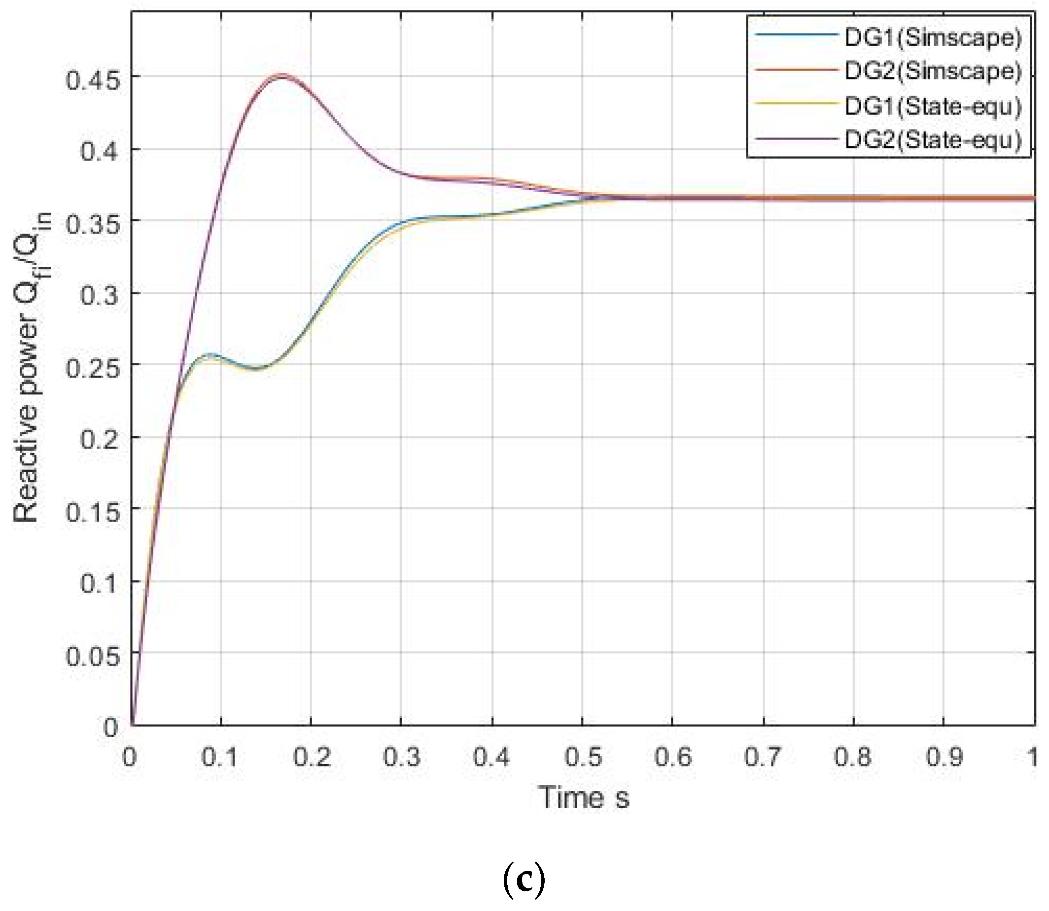
3.3. Validation of the State Model

The results concerning the evolution of the microgrid active and reactive powers, obtained under the same conditions using the Simscape model and the established state model, were used to validate the established state model. The same simulation scenario was considered for obtaining the simulation results using both models. Both DGs were connected to the microgrid at 0 s. The simulation results of both considered models are presented in Figure 12a,b, illustrating the evolution of the active and reactive powers of DG1 and DG2. Both models led to similar results; therefore, the established state model is considered validated. Thus, it can be used for studying the microgrid stability, integrating its control. To further confirm the validity of the developed model, Figure 12c shows a zoomed-in view of the transitory state after the connection of both DGs at 0 s.

4. Mesh Microgrid Stability and Robustness of its Control

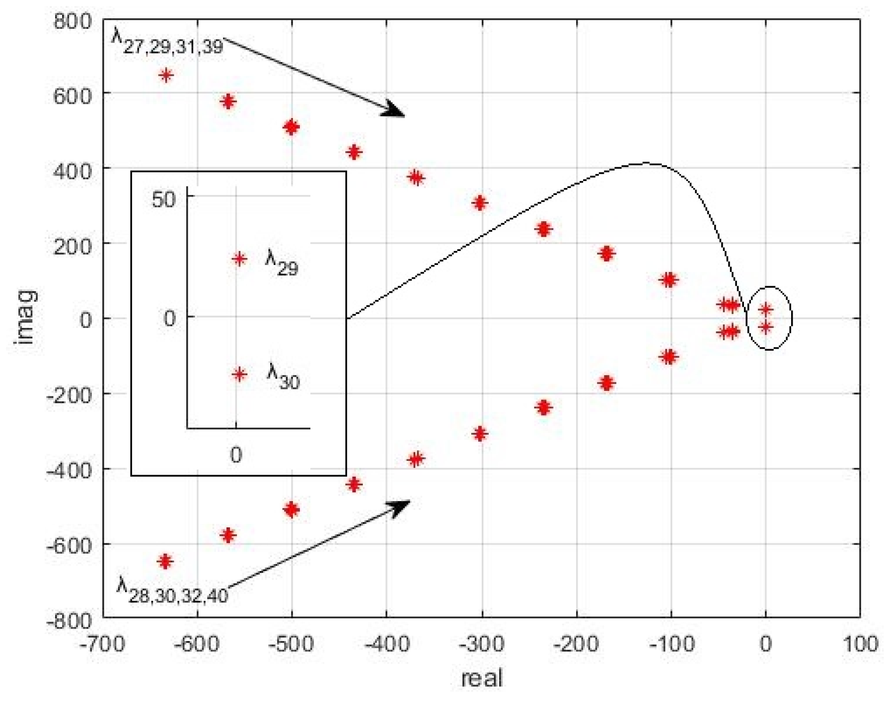
4.1. Jacobian Matrix Eigenvalues

In order to study the stability of the microgrid, defined by the continuous nonlinear differential system (24), and to analyze its dynamic behavior, which is affected by several control parameters, an eigenvalue sensibility analysis was performed by means of the calculation of the eigenvalues of the Jacobian matrix ${\left(\frac{\partial f}{\partial x}\right)}_{x_0}$ at the operating point $f\left(x_0\right)=0$. The system, i.e., the microgrid, will be asymptotically stable around the operating point $x_0$ if the real parts of all eigenvalues are strictly negative.

The system parameters are given in

Table 3. Parameters of the considered microgrid power lines.

Lines	Resistance (Ω)	Inductance (mH)	Capacitance (µF)	Points of Connection
Line 13	0.63	7.14	205	PCC1–PCC3
line 23	0.63	7.14	205	PCC2–PCC3
line 14	2.55	11.4	230	PCC1–PCC4
line 25	2	7	180	PCC5–PCC2
line 56	1.7	7.6	153.4	PCC5–PCC6
line 46	1.7	7.6	153.4	PCC4–PCC6

,

Table 4. Parameters of the considered microgrid power loads.

Serial RL Loads	Resistance (Ω)	Inductance (H)
Load 1	376.47	0.2496
Load 2	319.467	0.1765
Load 3	252.8977	0.1564
Load CPL	Pc = 100 KW	Qc = 0 VAR

and

Table 5. Parameters of the considered DGs.

DGs	Rated Active Power (MW)	Rated Reactive Power (Mvar)	Rated Phase to Phase Voltage (kV)	Cut-Off Frequency Power Calculation Filter (rad/s)	Cut-Off Frequency Second Order Filter (rad/s)	Damping Factor	Permissible Variations of Pulsation (for Droop Control)	Permissible Variations of Voltage (for Droop Control)
DG1	$P_{1n}=3$	$Q_{1n}=0.9$	$20$	${\omega }_{f1}=20$	${\omega }_{c1}=1000$	$\xi =0.7$	${\Delta }_{\omega }=0.5$	${\Delta }_E=6$
DG2	$P_{2n}=2$	$Q_{2n}=0.9$	$20$	${\omega }_{f2}=20$	${\omega }_{c2}=1000$	$\xi =0.7$	${\Delta }_{\omega }=0.5$	${\Delta }_E=6$

. The classical loads were modelled by serial R–L loads. The values of R and L were chosen depending on the operating point of these loads. The CPL was defined by constant values of its absorbed active and reactive powers, which may vary depending on its chosen operating point. The parameters of the DGs corresponded to their rated powers (available powers) and the parameters imposing the dynamic behavior of their control (${\omega }_f$, ${\omega }_c$, $\xi$, permissible variations of pulsation ${\Delta }_{\omega }$ and voltage ${\Delta }_E$).

The eigenvalues of the system at the considered operating point, corresponding to the parameters of the loads and DGs given in Table 4 and Table 5, are shown in

Table 6. Eigenvalues under nominal operating condition.

$\lambda$	$Value$
${\lambda }_{1,2}$	$-287\pm 37,510i$
${\lambda }_{3,4}$	$-287\pm 36,756i$
${\lambda }_{5,6}$	$-53\pm 26,120i$
${\lambda }_{7,8}$	$-54\pm 26,562i$
${\lambda }_{9,10}$	$-484\pm 26,915i$
${\lambda }_{11,12}$	$-484\pm 27,669i$
${\lambda }_{13,14}$	$-360\pm 15,598i$
${\lambda }_{15,16}$	$-360\pm 14,843i$
${\lambda }_{17,18}$	$-1766\pm 377i$
${\lambda }_{19,20}$	$-1488\pm 377i$
${\lambda }_{21,22}$	$-1564\pm 377i$
${\lambda }_{23,24}$	$-86\pm 377i$
${\lambda }_{25,26}$	$-254\pm 377i$
${\lambda }_{27,28}$	$-701\pm 714i$
${\lambda }_{29,30}$	$-700\pm 714i$
${\lambda }_{31,32}$	$-700\pm 714i$
${\lambda }_{33,34}$	$-9\pm 26i$
${\lambda }_{35}$	$-4.4089$
${\lambda }_{36}$	$-17.0790$
${\lambda }_{37}$	$-19.9387$
${\lambda }_{38}$	$-20.0041$
${\lambda }_{39,40}$	$-700\pm 714i$

. It can be observed that four of the Jacobian matrix eigenvalues are the negative real numbers, and that the other 36 eigenvalues are two by two the complex conjugate numbers, having negative real parts.

All of the Jacobian matrix eigenvalues have negative real parts, therefore the microgrid including its DG’s control and loads can be considered as a stable system around the considered operating point. The study of the considered mesh microgrid stability around other operating points can also be conducted based on the established state model.

In order to perform the sensitivity analysis and find the origin of different frequency components, depending on the parameters of the established model, the parameters of the different constituents of the microgrid, including its control parameters were modified separately. In the following sections, the evolution of eigenvalue trajectories with variation of the parameters of each microgrid constituent is discussed to verify their impact on the system stability.

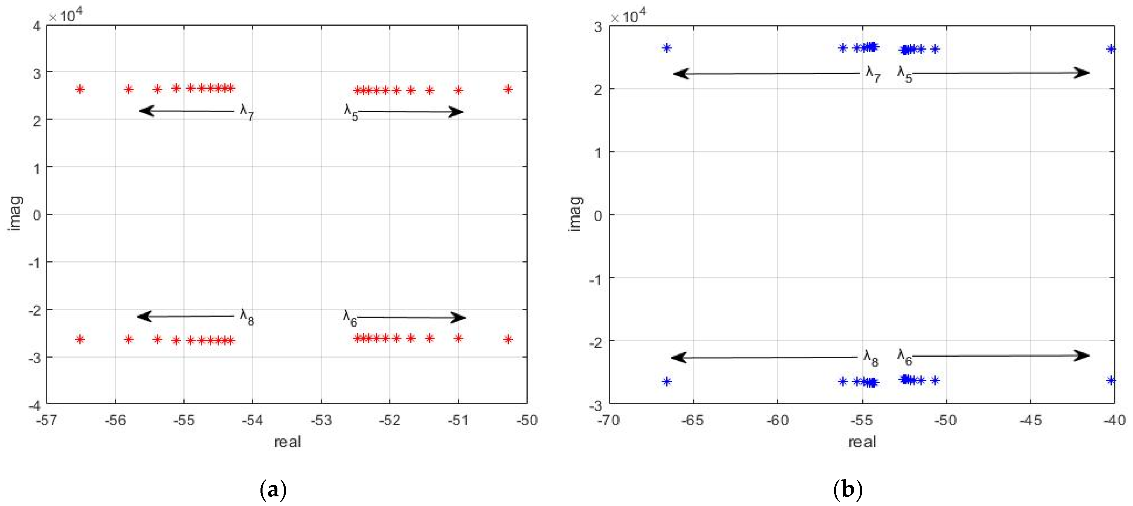
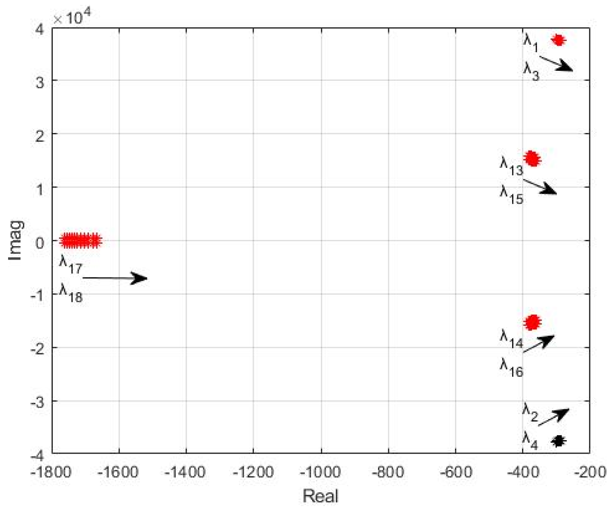
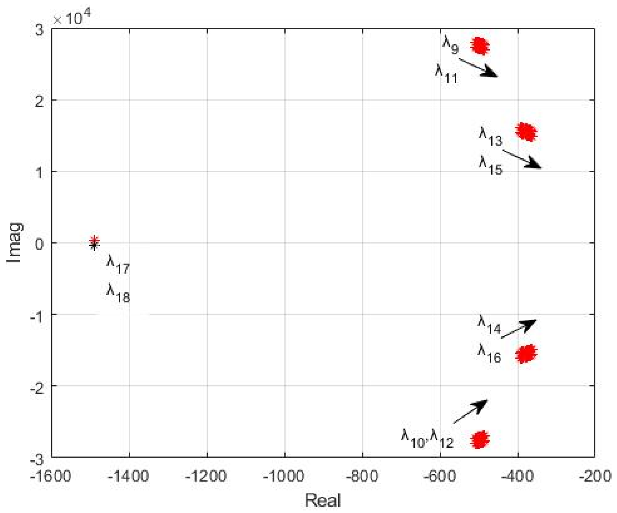
4.2. Eigenvalue Trajectory and Sensibility Analysis for Different Values of Power Line Parameters

To vary the parameters of the 6 power lines of the microgrid, the values of the lengths of all of these power lines are modified by 10 steps of 10% (for each line, from its initial length to two times this length), the Jacobean matrix eigenvalues are determined, and their evolution shown on Figure 13. The variation of the parameters of the power lines only impacts the eigenvalues ${\lambda }_1$ to ${\lambda }_{12}$, which are two by two complex conjugate numbers; the other eigenvalues ${\lambda }_{13}$ to ${\lambda }_{40}$ do not vary significantly with the evolution of the power line parameters. The real parts of the impacted eigenvalues (${\lambda }_1$ to ${\lambda }_{12}$) become closer to zero but remain sufficiently negative to not impact system stability when the line parameters are increased within the considered interval. However, if the lengths of the power lines become excessively long, the real parts of the impacted eigenvalues may become positives and cause system instability.

4.3. Eigenvalue Trajectory and Sensibility Analysis for Different Values of DG Parameters

The same approach as in Section 4.2. is used to study the impact of other parameters that may contribute to the instability of the system. For the considered DGs, the parameters which may impact the system stability are the cut-off frequency ${\omega }_f$ for power calculation (Equations (13) and (14)), the value of the filter’s cut-off frequency ${\omega }_c$ of the second order filter (Equation (15)), as well as the frequency drop ${\Delta }_{\omega }$ and the voltage drop ${\Delta }_E$ in Equations (6)–(8).

First, the cut-off frequency ${\omega }_f$ is modified in 10 steps (from its initial value to 10 times this value), the Jacobean matrix eigenvalues are determined, and their evolutions are illustrated in Figure 14. The variation of ${\omega }_f$ impacts the real negative eigenvalues ${\lambda }_{35}, {\lambda }_{36},{\lambda }_{37} \mathrm{and} {\lambda }_{38}$ as well as the eigenvalues ${\lambda }_{33},{\lambda }_{34}$ which are two complex conjugate numbers. The other eigenvalues do not vary significantly with the evolution of ${\omega }_f$. It can be seen that when ${\omega }_f$ increases, the eigenvalues ${\lambda }_{33}$, ${\lambda }_{34}$,${\lambda }_{36}$, ${\lambda }_{37}$ and ${\lambda }_{38}$ are shifted to the left while ${\lambda }_{35}$ moves very slightly toward zero, but its value does not change considerably and stays largely negative (from −4 to −3.6). The system always remains stable when ${\omega }_f$ increases, but the system dynamics become increasingly faster.

To examine the impact of ${\omega }_c$ in Equation (13), representing the delay imposed by the voltage source inverter (VSI) controlling the DG, on the system stability, its value is largely decreased (from its initial value 1000 rad/s to 50 rad/s). The eigenvalues most sensitive to the variation of ${\omega }_c$ are ${\lambda }_{27}$ to ${\lambda }_{32}$ as well as ${\lambda }_{39}$ and ${\lambda }_{40}$, which are two by two of the complex conjugate numbers. As shown in Figure 15, the real parts of the impacted eigenvalues move to the right when ${\omega }_c$ decreases and tend to be positive when ${\omega }_c$ becomes inferior to 50 rad/s, which causes the system instability.

To validate these results, the Simscape simulations were made to verify that any value of ${\omega }_c$ inferior to 50 rad/s can cause system instability. The results of the first simulation, made using the Simscape model with ${\omega }_c$= 50 rad/s, are illustrated on Figure 16a, and those of the second simulation with ${\omega }_{c }=45 \mathrm{rad}/s$ are shown on Figure 16b. These results confirm the system stability for ${\omega }_c$> 50 rad/s, as predicted by the stability analysis based on the established state model.

To evaluate the impact of droop control parameters on the system stability, the frequency drop ${\Delta }_{\omega }$ is increased in 10 steps (from its initial value to 10 times this value). The eigenvalues mostly impacted by this variation are ${\lambda }_{23}$ to ${\lambda }_{26}$ as well as ${\lambda }_{33}$ and ${\lambda }_{34}$ which are two by two complex conjugate numbers. As shown in Figure 17 when ${\Delta }_{\omega }$ increases the eigenvalues ${\lambda }_{23}$ to ${\lambda }_{26}$ move toward the left, while ${\lambda }_{33}$ and ${\lambda }_{34}$ move toward the right side of the real axis and become positive for ${\Delta }_{\omega } \ge 5$rad/s. By following the same approach as Simscape, simulations were made to verify that any value of ${\Delta }_{\omega }$ superior or equal to 5 rad/s can cause the system instability. The results of the first simulation, made using the Simscape model with ${\Delta }_{\omega } = 4.5$ rad/s, are illustrated In Figure 18a, and those of the second simulation with ${\Delta }_{\omega } = 5$ rad/s are shown In Figure 18b. These results confirm the system instability for ${\Delta }_{\omega } \ge 5$rad/s, as predicted by the stability analysis based on the established state model.

The voltage drop ${\Delta }_E$ is the last parameter of the DGs for which its impact on the system stability is studied. This has been done by varying ${\Delta }_E$ from its initial value to 10 times this value. The eigenvalues mostly impacted by this variation are ${\lambda }_{23}$ and ${\lambda }_{24}$, which are the complex conjugate numbers with a negative real part as well as ${\lambda }_{36}$ which is a real negative number. When the voltage drop increases, Figure 19 shows that ${\lambda }_{36}$ moves to the left while ${\lambda }_{23}$ and ${\lambda }_{24}$ move slightly to the right but remain negative. Thus, contrary to ${\Delta }_{\omega }$, the voltage drop ${\Delta }_E$ has a negligible impact on the system stability.

4.4. Eigenvalue Trajectory and Sensibility Analysis for Different Values of Load Parameters

In order to explain the effect of load variation on system stability, a study of the variation of dominant eigenvalue trajectories under different load conditions is established. Starting with the CPL type, Figure 20a,b show the trajectory of the eigenvalues under the effect of the change in active $P_c$ and reactive $Q_c$ powers absorbed by the CPL. As the active power or the reactive power absorbed by the CPL increases up to 120 kW (with fixed $Q_c=0$) and 72 kVAr (with fixed $P_c=100$ kW), respectively, the eigenvalues ${\lambda }_5$ to ${\lambda }_8$ are the most sensitive to the change of $P_c$ or $Q_c$ of the CPL. The other eigenvalues do not vary with the evolution of $P_c$ or $Q_c$. When the active power ($P_c$) absorbed by the CPL increases from 100 kW up to 120 kW (with fixed $Q_c=0$), the eigenvalues ${\lambda }_7$ and ${\lambda }_8$ move to the left far away from zero while ${\lambda }_5$ and ${\lambda }_6$ move toward the right but remain sufficiently negative. In the same manner, when the reactive power ($Q_c$) absorbed by the CPL increases from zero up to 72 kVAr (with fixed $P_c=100$ kW), the eigenvalues ${\lambda }_7$ and ${\lambda }_8$ move to the left while ${\lambda }_5$ and ${\lambda }_6$ move toward the right. For the considered intervals of the active power and reactive power, the real part of ${\lambda }_5$ and ${\lambda }_6$ remains sufficiently negative and the system stability is not affected. However, when the active power $P_c$ or the reactive power $Q_c$ become greater than certain limits, the real parts of the eigenvalues ${\lambda }_5$ and ${\lambda }_6$ become positive which causes system instability. For example, when $Q_c$ is fixed to zero, the limit value of active power $P_c$ absorbed by the CPL is 124.5 kW, beyond this value, the real part of the eigenvalues ${\lambda }_5$ and ${\lambda }_6$ becomes positive (Figure 21a for $P_c =124\mathrm{kW}$ and $P_c = 126\mathrm{kW}$) and the system cannot be considered asymptotically stable around the considered operating point. In the same manner, when $P_c$ is fixed to 100 kW, the limit value of reactive power $Q_c$ absorbed by the CPL is 74.3 kVAr; beyond this value, the real part of the eigenvalues ${\lambda }_5$ and ${\lambda }_6$ becomes positive (Figure 21b for $Q_c = 73 \mathrm{kVAr}$ and $Q_c = 74 \mathrm{kVAr}$).

To confirm the results concerning the stability limits imposed by the CPL, the Simscape simulations were made for two values of the CPL active power, one less than the active power limit ($P_c = 124 \mathrm{kW}$) and another one higher than this limit ($P_c = 125\mathrm{kW}$) and the results are shown in Figure 22a,b. These results are in perfect accordance with the conclusions drawn from the established state model relating to the impact of the CPL on the stability of the considered system.

In order to maintain the microgrid stability for higher values of active power absorbed by the CPL, one solution consists of adding a capacitor to the PCC to which the CPL is connected. Then, the established state model can be used to dimension the necessary capacitor value for the required CPL active power. For the considered microgrid, the CPL is connected to PCC3, and based on the above analysis, the system stability is affected when the CPL active power becomes higher than 124$\mathrm{kW}$. The latter active power limit can be augmented; for example, to $P_c$= 620$\mathrm{kW}$ by imposing an adapted value to the capacitor connected to PCC3. This value can be determined using the established state model.

When $Q_c=0$, the limit value of active power $P_c$ absorbed by the CPL becomes 620 kW when the capacitor $c_3$ is modified from 0.4 µF to 2 µF. Figure 23 shows that the real part of the eigenvalues ${\lambda }_5$ and ${\lambda }_6$ is negative for $P_c=620 \mathrm{kW}$ and positive for $P_c=625 \mathrm{kW}$. Then the microgrid stability is ensured up to $P_c=620 \mathrm{kW}$. This result is in perfect accordance with the Simscape simulation results shown in Figure 24a,b. Hence, the stability analysis based on the established state model can be used as a powerful tool to adjust mesh microgrids to guarantee their stability when their loads or even their architectures change.

Concerning the serial R–L loads in the microgrid, the impact of their variations on the system stability is studied by analyzing the evolution of the eigenvalues mostly impacted by the change under constant power factor of each RL-load connected to a given PCC. In fact, the power factor of classical loads is usually higher than 0.92 and its variation can be neglected. For the three serial RL-loads of the considered microgrid shown in Figure 10, Figure 25, Figure 26 and Figure 27 show the evolution of the eigenvalues mostly impacted by varying (from initial value to 50% of this value) the impedances of RL-load3, RL-load4 and RL-load5 under constant power factor, respectively. The most impacted eigenvalues in this case are ${\lambda }_1$ to ${\lambda }_{12}$, which correspond to line current equations and ${\lambda }_{13}$ to ${\lambda }_{20}$ as well as ${\lambda }_{25}$ and ${\lambda }_{26}$, which correspond to the PCC voltage equations. It can be noticed that when the value of each RL-load decreases under constant power factor, the eigenvalues mostly impacted move to the right but remain sufficiently negative and do not impact the system stability as long as the load variation is within the indicated power range.

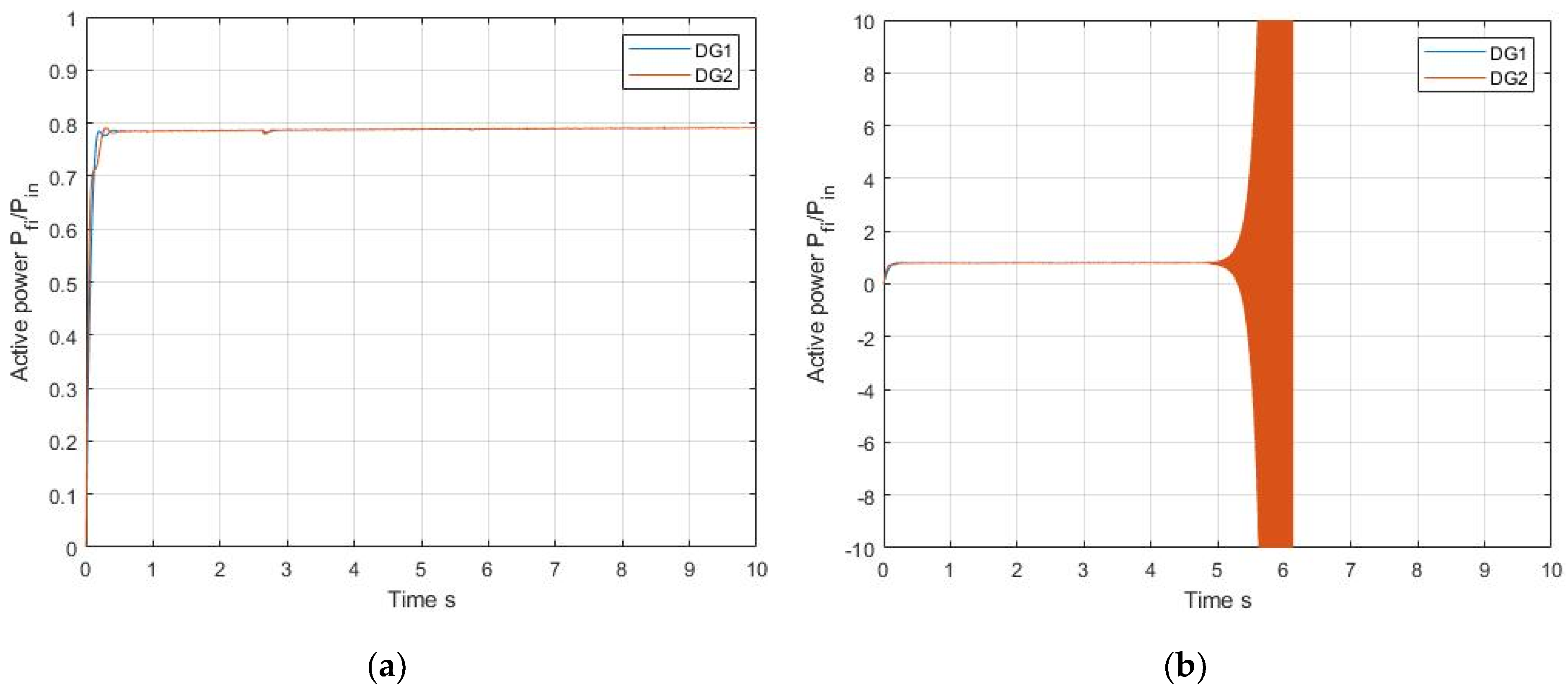
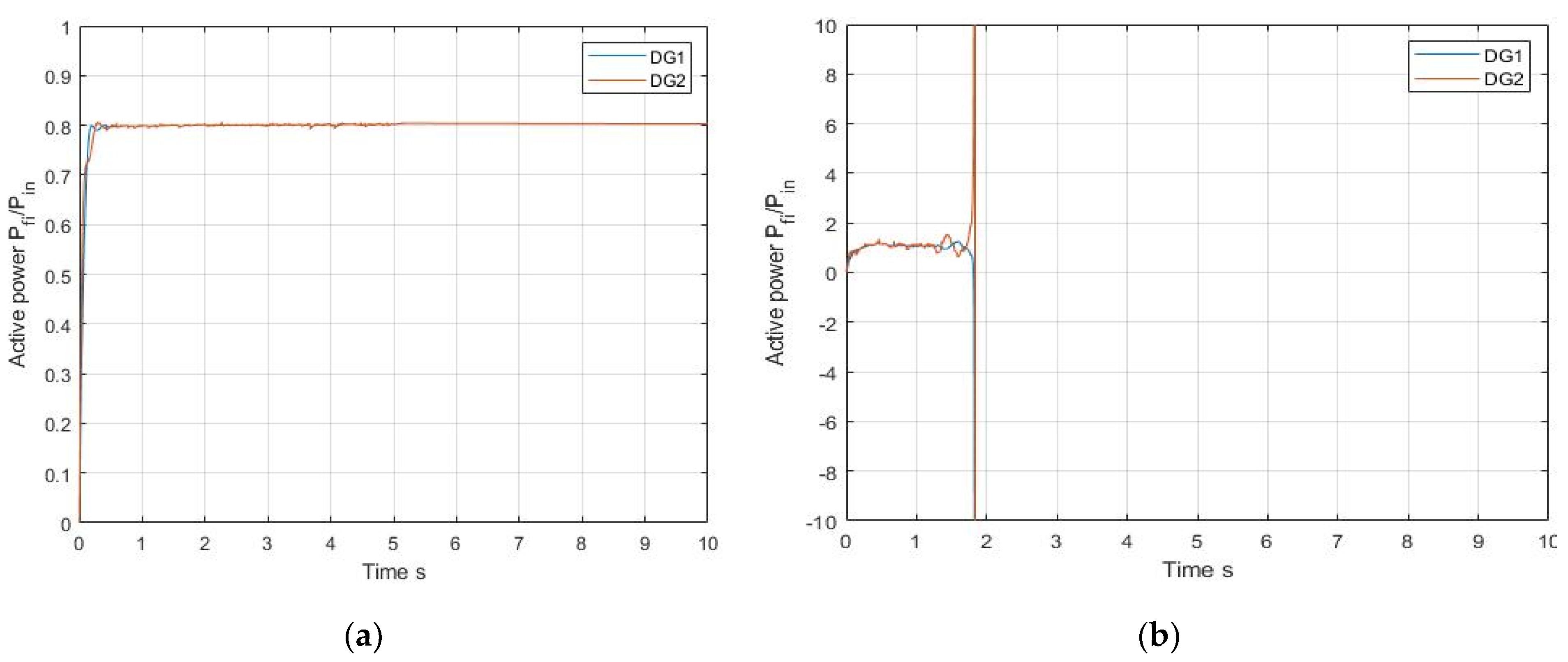
4.5. Mesh Microgrid Control Robustness

Based on the established and validated state-model, including the modified droop-control that ensures active and reactive power sharing, the considered mesh microgrid control robustness with respect to the modifications caused by the connection of DGs and large load variations is studied. In this simulation, at 0 s, the first DG sets the frequency of the microgrid and the voltages of the PCCs while only the first RL load is connected. Then, the second DG is interconnected to the microgrid at 5 s after being synchronized from 1 s to 5 s. At 8 s, the second RL load is also connected, applying a high positive load step to the microgrid. Finally, at 11 s, the CPL load absorbing an active power of 100 kW is also connected to the microgrid to verify its effect on the active and reactive power sharing.

Due to the modified droop control strategy given by Equations (9) and (10), the active and reactive power sharing is ensured (Figure 28a,b). The convergence of the reactive power of the two DGs under different load conditions is convincingly verified in Figure 28b. In addition, and as foreseen by the stability analysis based on the state-model, the microgrid stability is ensured in different microgrid structure configuration when the CPL active power load does not exceed 124 kW.

5. Discussion

An improved droop control strategy for synchronization and power sharing was applied on a mesh multi-PCC islanded microgrid. With only the information on the measured RMS voltage value at a pilot node, this strategy has proven its efficiency for fast synchronization as well as active and reactive power sharing between all microgrid DGs. This makes the mesh multi-PCC microgrid eligible to the “plug and play” feature.

In order to study the microgrid stability and its droop control robustness, a state model of the complete system has been proposed and validated based on simulation results achieved using both the Simscape model and proposed state-model. Then, the stability analysis of the considered non-linear system at each operating point was performed using the Jacobean matrix of the state model. In practice, the dynamic behavior of different state variables and the origin of different frequency components were found by studying the evolution of the system eigenvalues with respect to the parameters of the power lines, DGs and different loads. It was found that the most influent system parameters on its stability were the DGs control parameters and the CPL active power level.

In addition, it has been shown through an example that the established state model, which allows the study of system stability, can be used as a powerful tool to adjust certain mesh microgrid parameters to guarantee its stability when the absorbed active power level of its CPLs becomes too high. Finally, the validated microgrid state-model, including the modified droop-control that ensures active and reactive power sharing, also achieved mesh microgrid control robustness with respect to the modifications caused by the connection of DGs and large load variations, which means that the new droop control is always effective under different network configurations.

The developed modified droop control strategy can be adapted and used for power sharing in grid-connected mesh microgrids, and the synchronization strategy can also be adapted for a seamless transfer from an islanded microgrid to a grid-connected microgrid. As mentioned in the Introduction, the developed and validated state-space model can be the base for many future studies in mesh microgrids.

References

1. El-Khattam, W.; Salama, M.M. Distributed generation technologies, definitions and benefits. Electr. Power Syst. Res. 2004, 71, 119–128. [Google Scholar] [CrossRef]
2. Zhang, L.; Harnefors, L.; Nee, H.-P. Power-Synchronization Control of Grid-Connected Voltage-Source Converters. IEEE Trans. Power Syst. 2010, 25, 809–820. [Google Scholar] [CrossRef]
3. Haizhen, X.; Xing, Z.; Fang, L.; Debin, Z.; Rongliang, S.; Hua, N.; Wei, C. Synchronization strategy of microgrid from islanded to grid-connected mode seamless transfer. In Proceedings of the IEEE International Conference of IEEE Region 10 (TENCON 2013), Xi’an, China, 22–25 October 2013. [Google Scholar]
4. Tayaba, U.B.; Roslan, M.A.B.; Hwai, L.J.; Kashif, M. A review of droop control techniques for microgrid. Renew. Sustain. Energy Rev. 2017, 76, 717–727. [Google Scholar] [CrossRef]
5. Xiaofei, X.; Hong, L.; Zhipeng, L. Research on new algorithm of droop control. In Proceedings of the Chinese Control and Decision Conference (CCDC), Guiyang, China, 25–27 May 2013. [Google Scholar]
6. Huang, X.; Wang, K.; Qiu, J.; Hang, L.; Li, G.; Wang, X. Decentralized Control of Multi-Parallel Grid-Forming DGs in Islanded Microgrids for Enhanced Transient Performance. IEEE Access 2019, 7, 17958–17968. [Google Scholar] [CrossRef]
7. Han, H.; Hou, X.; Yang, J.; Wu, J.; Su, M.; Guerrero, J.M. Review of Power Sharing Control Strategies for Islanding Operation of AC Microgrids. IEEE Trans. Smart Grid 2016, 7, 200–215. [Google Scholar] [CrossRef] [Green Version]
8. Moussa, H.; Shahin, A.; Martin, J.-P.; Pierfederici, S.; Moubayed, N. Optimal angle droop for power sharing enhancement with stability improvement in islanded microgrids. IEEE Trans. Smart Grid 2017, 9, 5014–5026. [Google Scholar] [CrossRef]
9. Dheer, D.K.; Kulkarni, O.V.; Doolla, S.; Rathore, A.K. Effect of Reconfiguration and Meshed Networks on the Small-Signal Stability Margin of Droop-Based Islanded Microgrids. IEEE Trans. Ind. Appl. 2018, 54, 2821–2833. [Google Scholar] [CrossRef]
10. Trivedi, A.; Singh, M. Adaptive Droop Control for AC Microgrid with Small Mesh Network. IEEE Trans. Ind. Electron. 2018, 65, 4781–4789. [Google Scholar] [CrossRef]
11. Zhu, Y.; Zhuo, F.; Shi, H. Accurate power sharing strategy for complex microgrid based on droop control method. In Proceedings of the IEEE 10th International Symposium on Power Electronics for Distributed Generation Systems (PEDG), Xi’an, China, 3–6 June 2019. [Google Scholar]
12. Jiao, J.; Guo, S.; Tan, C.; Xue, Y.; Hua, X. Research on Improved Droop Control Method of DC Microgrid Based on Voltage Compensation. In Proceedings of the 2020 5th International Conference on Power and Renewable Energy (ICPRE), Shanghai, China, 12–14 September 2020; pp. 391–395. [Google Scholar] [CrossRef]
13. Jusoh, A.B. The instability effect of constant power loads. In Proceedings of the National Power and Energy Conference PECon 2004, Kuala Lumpur, Malaysia, 29–30 November 2004; pp. 175–179. [Google Scholar]
14. Cespedes, M.; Xing, L.; Sun, J. Constant-power load system stabilization by passive damping. IEEE Trans. Power Electron. 2011, 26, 1832–1836. [Google Scholar] [CrossRef]
15. Marx, D.; Magne, P.; Nahid-Mobarakeh, B.; Pierfederici, S.; Davat, B. Large signal stability analysis tools in DC power systems with constant power loads and variable power loads—A review. IEEE Trans. Power Electron. 2012, 27, 1773–1787. [Google Scholar] [CrossRef]
16. Kabalan, M.; Singh, P.; Niebur, D. Large signal Lyapunov-based stability studies in microgrids: A review. IEEE Trans. Smart Grid 2016, 8, 2287–2295. [Google Scholar] [CrossRef]
17. Bottrell, N.; Prodanovic, M.; Green, C.T. Dynamic stability of a microgrid with an active load. IEEE Trans. Power Electron. 2013, 28, 5107–5119. [Google Scholar] [CrossRef] [Green Version]
18. Rasheduzzaman, M.; Mueller, J.A.; Kimball, W.J. An accurate small-signal model of inverter- dominated islanded microgrids using dq reference frame. IEEE J. Emerg. Sel. Top. Power Electron. 2014, 2, 1070–1080. [Google Scholar] [CrossRef]
19. Hennane, Y.; Martin, J.; Berdai, A.; Pierfederici, S.; Meibody-Tabar, F. Power Sharing and Synchronization Strategies for Multiple PCC Islanded Microgrids. Int. J. Electr. Electron. Eng. Telecommun. 2020, 9, 156–162. [Google Scholar] [CrossRef]
Figure 1. Microgrid with one point of common coupling (PCC).
Sustainability 13 02243 g001
Figure 2. IEEE 9 bus test feeder.
Sustainability 13 02243 g002
Figure 3. Evolution of the distributed generator (DG) active (a) and reactive (b) powers (first DG supplies the microgrid up to 5 s, the second DG is connected to the microgrid at 5 s).
Sustainability 13 02243 g003
Figure 4. Scheme of the controllable voltage sources DG1 and DG2.
Sustainability 13 02243 g004
Figure 5. Equivalent synoptic diagram describing a droop-controlled DGi.
Sustainability 13 02243 g005
Figure 6. Evolution of the DG active (a) and reactive (b) powers (first DG supplies the microgrid up to 5 s, the second DG is connected to the microgrid at 5 s).
Sustainability 13 02243 g006
Figure 7. Evolution of the DG active (a) and reactive (b) powers (both DGs are connected at 0 s).
Sustainability 13 02243 g007
Figure 8. Evolution of the DG active power under different state of charge (first DG supplies the microgrid up to 5 s, the second DG is connected to the microgrid at 5 s).
Sustainability 13 02243 g008
Figure 9. Equivalent synoptic diagram describing a droop-controlled DGi.
Sustainability 13 02243 g009
Figure 10. IEEE 9bus test feeder.
Sustainability 13 02243 g010
Figure 11. Reference frames α β and d q.
Sustainability 13 02243 g011
Figure 12. Simulation results obtained using Simscape and the mathematical state-model. Both DGs were connected to the microgrid at 0 s. (a) Evolution of the DGs per unit active powers. (b) Evolution of the DGs per unit reactive powers. (c) Zoomed-in view of the per unit reactive powers around 0 s.
Sustainability 13 02243 g012aSustainability 13 02243 g012b
Figure 13. Evolution of eigenvalues corresponding to the change in line parameters.
Sustainability 13 02243 g013
Figure 14. Evolution of eigenvalues corresponding to the change in ω f ( 20 < ω f < 200 ( rad / s ) with ω f increasing).
Sustainability 13 02243 g014
Figure 15. Evolution of eigenvalues corresponding to the change in ω c ( 50 < ω c < 1000   ( rad / s ) with ω c decreasing).
Sustainability 13 02243 g015
Figure 16. Evolution of the DG active power (Simscape model (both DGs are connected at 0 s)): (a) with ω c = 50   rad / s . (b) with ω c = 45   rad / s .
Sustainability 13 02243 g016
Figure 17. Evolution of eigenvalues corresponding to the change in Δ ω ( 0.5   <   Δ ω   <   5.5   ( rad / s ) ) with Δ ω increasing.
Sustainability 13 02243 g017
Figure 18. Evolution of the DGs active power (Simscape model, both DGs connected at 0 s): (a) Δ ω   = 4.5 rad/s and (b) Δ ω   = 4.5.
Sustainability 13 02243 g018
Figure 19. Evolution of Eigenvalues with the change in voltage drop 6   <   Δ E   <   70 ( V ) with Δ V increasing.
Sustainability 13 02243 g019
Figure 20. Evolution of eigenvalues with the change of the CPL active and reactive power: (a) P c increasing 100 ( kW )   <   P c   <   120 ( kW ) and Q c   =   0 ; (b) Q c increasing 0   <   Q c   <   72 ( kVAr ) and P c   =   100   kW .
Sustainability 13 02243 g020
Figure 21. Evolution of the eigenvalues with the change of the CPL active or reactive power around their limited values: (a) active power variation from P c   =   124   kW to P   c =   126   kW when Q c   =   0 ; (b) reactive power variation from Q c   =   73   kVAr to Q c   =   74   kVAr when P c   =   100   kW .
Sustainability 13 02243 g021
Figure 22. Evolution of the DGs active power (Simscape model with both DGs connected at 0 s): (a) P c = 124   kW . (b) P c = 125   kW .
Sustainability 13 02243 g022
Figure 23. Evolution of the eigenvalues with the change of the CPL active power around its limited value from P c = 620   kW to P c = 625   kW when Q c = 0 .
Sustainability 13 02243 g023
Figure 24. Evolution of the DGs active power (Simscape model with both DGs connected at 0 s): (a) P c     = 620   kW . (b) P c   = 625   kW .
Sustainability 13 02243 g024
Figure 25. Evolution of eigenvalues corresponding to the decrease in RL-load3 under constant power factor: 175   <   R Load 3   <   376 ( Ω ) and 0.13   <   L Load 3   <   0.25 ( H ) .
Sustainability 13 02243 g025
Figure 26. Evolution of eigenvalues corresponding to the decrease in RL-load4 under constant power factor:   155 < R Load 4 < 319 ( Ω ) and 0.085 < L Load 4 < 0.17 ( H ) .
Sustainability 13 02243 g026
Figure 27. Evolution of eigenvalues corresponding to the decrease in RL-load5 under constant power factor: 126 < R Load 5 < 252 ( Ω ) and 0.077 < L Load 5 < 0.1564 ( H ) .
Sustainability 13 02243 g027
Figure 28. Evolution of the DG active (a) and reactive (b) powers under different states of charge.
Sustainability 13 02243 g028