Sustainable Fault Diagnosis of Imbalanced Text Mining for CTCS-3 Data Preprocessing

Abstract

At present, the method for fault diagnosis and maintenance of the CTCS-3 (Chinese Train Control System Level 3) electronic equipment relies too heavily on expert knowledge. Moreover, the use of historical fault data is not valued. This paper proposes a sustainable fault diagnosis model based on imbalanced text mining. First, to process fault data from the field recorded in natural language, natural language processing technology is used to extract fault feature words. Then, a term frequency-inverse document frequency model is used to transform the fault feature words extracted from the database into vectors. It is worth noting that imbalance in the fault samples affects the accuracy of this sustainable fault diagnosis model. To solve this problem, we use the borderline-synthetic minority over-sampling technique in the step of predicting train fault components, we also use the backpropagation neural network we proposed and the naive Bayesian model which is commonly used as a classification model, to compare the prediction accuracy of these two algorithms. The experimental results perform well, which proves that the fault diagnosis method using the backpropagation neural network can further assist engineers to complete timely repair and maintenance work. The research in this paper has played a very important role in technical support for intelligent train dispatching and command, and will also play a positive role in technical support for the automatic operation of urban rail transit under the prevention and control of the new coronavirus.

1. Introduction

China’s railway construction and technological development have made gratifying achievements, such as the rapid extension of railway operation mileage, continuous improvement of train speeds, and the gradual increase of train operation density. However, if a train accident was to occur in this high-density and high-speed environment, the consequences would be catastrophic. With the continuous development of communication technology, computer technology, and electronic information technology, decentralized and self-regulating centralized dispatching systems are increasingly being perfected. With their unique advantages, such systems play an important role in modern railway transportation command.

The Chinese Train Control System Level 3 (CTCS-3) is widely used in Chinese high-speed railways, and it is a safety-critical system for train operation. If one of the modules fails, a threat is posed to train operation safety. Therefore, timely and effective fault detection and maintenance are particularly important. However, many faults cannot be diagnosed on the basis of their fault phenomenon. When a fault occurs, the corresponding fault phenomenon can only be recorded by the drivers, and the faulty components are repaired when the train returns to the depot, leading to a long fault diagnosis cycle and affecting the operational efficiency of the railway. Hence, the study of train control system failures is particularly important for the efficient operation of the entire railway transportation system.

Many fault diagnosis methods have been developed for train control systems in recent years. For certain specific component failures, Shangguan Wei et al. [1] proposed a method that combines rough set theory and a neural network algorithm. This method overcomes the weakness of neural networks when dealing with high-noise data, and has been applied to the fault diagnosis process of the on-board Balise transmission module (BTM) unit. Zihui Zuo et al. [2] proposed a fault diagnosis method based on an adaptive neuro-fuzzy inference system and use it in the wireless connection timeout fault diagnosis process of the CTCS. Jiang Liu et al. [3] proposed a rule-based fault diagnosis approach that detects the characteristics of different fault modes in the speed and distance unit, identifies the fault and offers suggested maintenance measures.

Fault diagnosis methods based on Bayesian networks are often used in fault detection over the entire CTCS. Jingjing Zhao et al. [4] proposed a Bayesian fuzzy inference net real-time internal fault diagnostic system for the CTCS-3 train control system, and their experimental results verified the effectiveness and feasibility of the method. Xiao Liang et al. [5] proposed a fault diagnosis method based on a Bayesian network. With the reduction of fault symptoms based on rough set theory, the complexity of the training model is reduced. Further, with a combination of expert knowledge and fault data training, the improved Bayesian network integrates the correlation between the fault symptoms into the model. Yu Cheng et al. [6] proposed a fault diagnosis model based on a dynamic Bayesian network for high-speed train control systems. The maintenance data of a high-speed train control system was used to verify the feasibility of the proposed algorithm.

For data preprocessing, Bin Chen et al. [7] analyzed the fault data of on-board systems recorded in natural language using text mining. A custom dictionary was constructed for word segmentation, and because these authors used the character matching method, fault text chains, and the construction method were defined in order to process the fault recording files. Wang Feng et al. [8] proposed a bilevel feature extraction-based text mining method that integrates features extracted at both syntax and semantic levels with the aim to improve the fault classification performance and to adapt to the text recording method of fault data in the railway maintenance industry. Qi Kang et al. [9] proposed a new under-sampling scheme by incorporating a noise filter before executing resampling. Furthermore, this paper also summarized the relationship between data imbalanced ratio and algorithm performance. Q. Kang et al. [10] proposed a distance-based weighted under-sampling scheme for support vector machines. However, most methods only analyze specific fault types or only focus on the fault diagnosis process without preprocessing the data, as this is not useful for the maintenance of the railway system.

Different fault detection methods are also applied to other devices. Himadri Lala et al. [11] used an empirical mode decomposition (EMD)-based approach along with an artificial neural network (ANN) for the analysis of real-time arc signals. The results obtained by the application of EMD and ANN successfully classified the arcing events by support vector machine and Kth nearest neighbor machine learning techniques. Kou Lei et al. [12] proposed a fault diagnosis method based on a deep feedforward network to reduce the dependence on the fault mathematical models. Xiaoyue Yang et al. [13] proposed an optimal fractional-order method for transient fault diagnosis in the traction control system which can suppress background noise and amplifies the faulty party of the signal. In [14], a knowledge-driven and data-driven novel fault diagnosis approach was proposed The robustness performance of the sustainable fault diagnosis classifier is improved by using Concordia transform and random forests fault technique. Zhongxu Hu et al. [15] proposed a new data-driven fault diagnosis method based on compressed sensing (CS) and improved multiscale network (IMSN). CS is used to reduce the amount of raw data, and the IMSN is established for learning and obtaining deep features. In [16], a group of long short-term memory (LSTM) models were trained by a time-series representation of the vibration signal collected from a compressor. Compared with classical approaches, the LSTM-based model shows a remarkable improvement in performance. Tao Zhou et al. [17] proposed a model that merges a weighted score fusion scheme into the deep neural network to adaptively determine the optimal weights for each feature stream. Lu Wei et al. [18] proposed a new normal behavior modeling (NBM) method to predict wind turbine electric pitch system failures using supervisory control and data acquisition (SCADA) information. K. Zhong et al. [19] presented a systematic overview of data-driven fault prognosis for industrial systems. According to different data characteristics, corresponding failure prediction methods are explained.

The fault diagnosis proposed in this paper is one of the important artificial intelligent technologies. This paper takes the initiative in putting forward a data preprocessing method for real-time fault diagnosis and location by the CTCS-3 on-board system. First, fault data recorded in the natural language form is processed by NLP (Natural Language Processing) to extract fault feature words. Then, the term frequency-inverse document frequency (TF-IDF) weighting method is used to vectorize the fault data according to the extracted fault features. Due to the imbalanced characteristics of the data, the borderline-synthetic minority over-sampling technique (SMOTE) algorithm is then used to synthesize the data in the minority sample set to improve the accuracy of the results. Finally, a backpropagation (BP) neural network is used to predict the fault components as a classifier. This paper proves the feasibility of the model and demonstrates its efficacy in fault diagnosis.

2. Data Resources

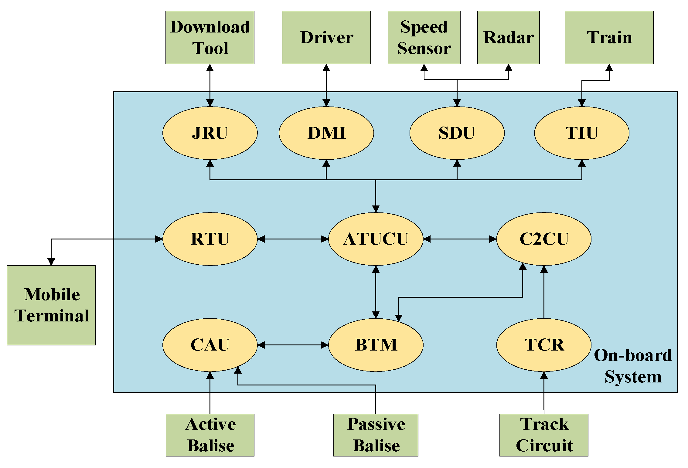
The system structure of the fault data streams from the CTCS-3 physics architecture is shown in Figure 1. The Vital Computer Unit (VCU), BTM, Track Circuit Reader (TCR), Speed and Distance unit (SDU), Driver-Machine Interface (DMI), Train Interface Unit (TIU), Juridical Recorder Unit (JRU), GSM-R Wireless Communication Unit (RTU), Vital Digital Input/Output (VDX), Safe Transmission Unit (STU-V) and other units work together to complete the functions of the on-board system. The VCU includes the CTCS-3 level control unit (ATPCU), the CTCS-2 level control unit (C2CU), Speed and Distance Process (SDP), and the Train Security Gateway (TSG). The Train Interface Equipment (TIE) includes VDX, the Multifunction Vehicle Bus (MVB), relay, and so on, and implements data transfer and information exchange. In this paper, Compact Antenna Unit (CAU) faults are classified as BTM faults.

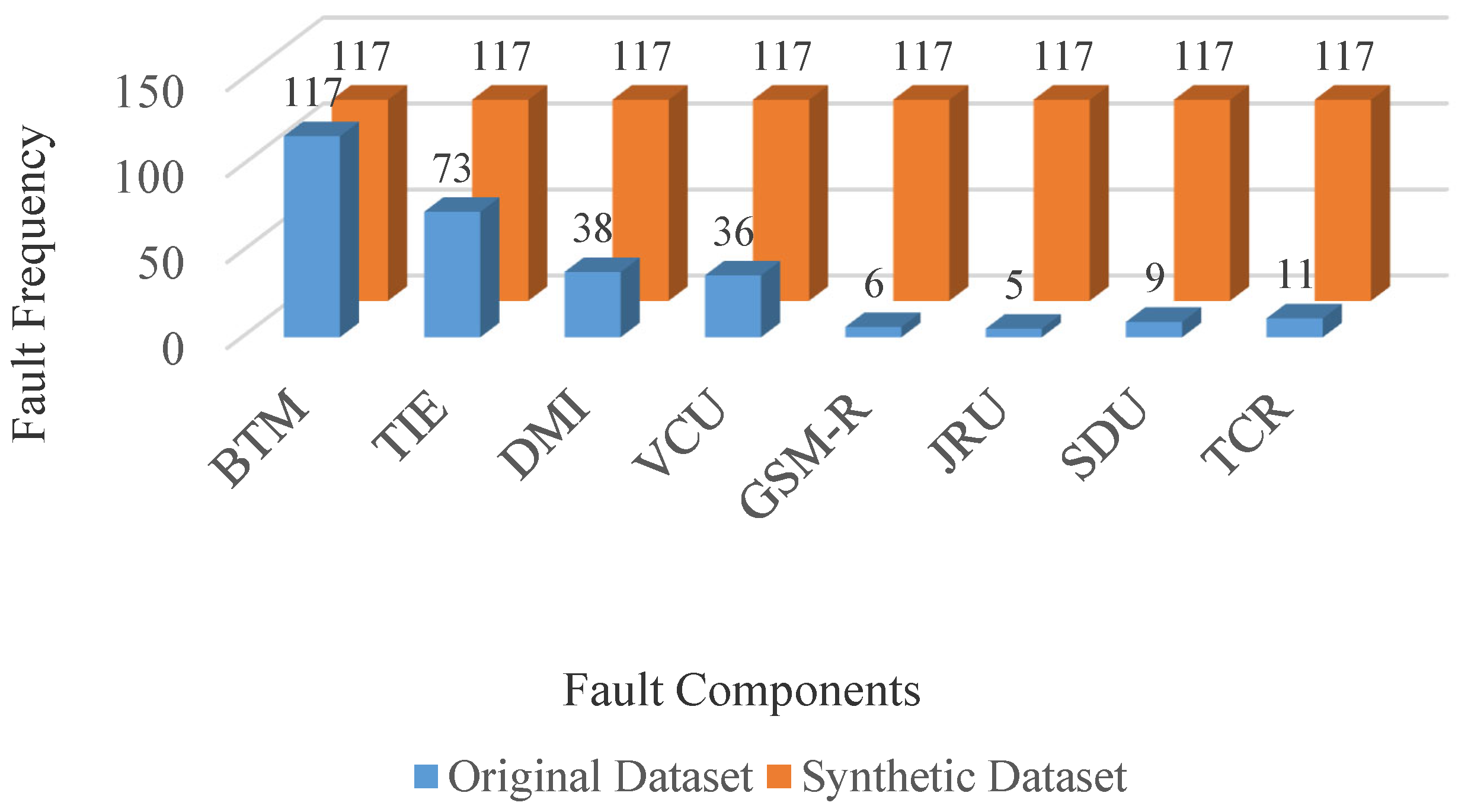
From the existing 295 fault data of the fault data streams from the CTCS-3 physics architecture, fault components are mainly divided into the following eight categories; the corresponding fault components and failure frequencies are shown in Figure 2.

3. Natural Language Processing

In the collection and storage of fault data streams from the CTCS-3 physics architecture, there are fewer samples for the parameters of the same system unit, and the error characteristics of the data obtained are not obvious. If the original data processing (such as signal estimation and detection, parameter operation, etc.) cannot generate the correct feature analysis and classification, this may result in misjudgment and incorrect operation of the CTCS-3. To reduce bias and improve the consistency and effectiveness of the system data identification, automatic preprocessing of the data sourced from the CTCS-3 is necessary.

Fault data from train control systems are primarily recorded by field staff and maintenance engineers in natural language form. These records, as shown in

Table 1. Fault records.

Number	Fault Description	Faulty Component	Causes of Failure	Treatment
1	When the GXXXX train was driving at 7:30 in XXX station, the driver reported that the communication between Host and DMI is interrupted, the ATP (Automatic Train Protection) crashed, and could not start normally multiple times	Train interface unit	Emergency BFB (Brake Feedback Relay) failure	Replace the faulty relay

, include the time and place of the fault that occurred, the train number, a description of the fault phenomenon, and the faulty components. Since the fault data described in natural language has no uniform format, it is difficult for the computer to directly analyze its semantics and process it accordingly. Therefore, preprocessing the fault data is the first problem to be solved.

Text preprocessing is the basis of feature extraction. First, a custom thesaurus is constructed based on expert knowledge, then the stop words dictionary is built, as shown in

Table 2. Demonstration of stop words dictionary and custom dictionary.

Stop Word Dictionary	Custom Dictionary
And	Balise message error
Beijing	Speed sensor failed
Guangzhou	Host and DMI communication is interrupted
Block	Restart and recovery
Driver	Braking test failed

. The custom thesaurus is necessary to supplement the segmentation dictionary in the process of Chinese word segmentation and guarantees the accuracy of the segmentation when encountering professional words. The stop words dictionary is used to delete the words irrelevant to fault features. The fault text is then segmented into discrete entries according to the segmentation dictionary. Meanwhile, the stop words in the lexicon are removed and the feature words are retained. Finally, the related synonyms are merged, and the frequency of words is calculated to obtain the feature lexicon. Because there is an enormous number of feature words in the feature lexicon after segmentation, expert knowledge and word frequency can be used to screen out feature words that may represent fault symptoms. The feature lexicon is shown in

Table 3. Fault feature words.

Number	Feature Words	Number	Feature Words
1	ATP failure	13	Cannot start normally
2	ATP crash	14	From C3 to C2
3	Change system to restart	15	Blank screen
4	BTM failure	16	Balise message missing
5	Balise message error	17	JRU failure
6	Trigger emergency brake	18	SDU failure
7	Parking	19	Speed sensor failure
8	Communication between host and DMI is interrupted	20	Common brake failure
9	CTCS-2 failure	21	Braking test failed
10	ATPCU failure	22	Wireless connection Timeout
11	Trigger common brake	23	Braking
12	Message full of zeros from Balise	24	TCR failure

.

4. Feature Extraction and Vectorization

In this section, all of the fault texts are vectorized using the TF-IDF technique based on the keywords extracted above, and 295 24-dimensional vector data are generated. TF-IDF is a common statistical weighting method, widely used in information retrieval and text analysis. TF denotes “term frequency”, that is, the frequency of entries appearing in the text. In this study, the entries are the 24 fault feature words extracted above. The process can be presented as:

$$T{F}_{i,j}=\frac{n_{i,j}}{{{\displaystyle \sum }}_k{n}_{k,j}+1}$$

(1)

where $n_{i,j}$ is the number of times the word $w_i$ appears in the document $d_j$ and ${\displaystyle \sum }_k{n}_{\begin{array}{c}k,j\\ \end{array}}$ is the sum of the occurrences of all the words in the document $d_j$. Adding 1 to the denominator is to keep the denominator from being zero.

IDF indicates the inverse document frequency. The formula is as follows:

$$ID{F}_i=log\frac{N}{k_i+1}$$

(2)

where $k_i$ is the number of documents containing the word $w_i$ and $N$ is the number of documents in corpus D. Adding 1 to the denominator is to avoid the case where the denominator is zero.

Combing the term frequency and the inverse document frequency, which means using $ID{F}_i$ to adjust $T{F}_{i,j}$, yields the weight of the word $w_i$ in the document $d_j$:

$$W_{j,i}=T{F}_{i,j}\times ID{F}_i$$

(3)

Each document can form a vector with the word weight of the fault feature words.

$$d_j=\left[W_{j,1} W_{j,2} W_{j,3 }\cdots W_{j,n}\right]$$

(4)

After the above steps, 295 text data become the following matrix:

$$W_{j,i}={\left[\begin{array}{cccccccccc}0& 0.180& 0.150& 0& 0.106& 0& \cdots & 0& 0.199& 0\\ 0.145& 0& 0& 0& 0.084& 0& \cdots & 0& 0& 0.286\\ 0& 0& 0& 0.233& 0.103& 0& \cdots & 0& 0& 0\\ ⋮& ⋮& ⋮& ⋮& ⋮& ⋮& \ddots & ⋮& ⋮& ⋮\\ 0.131& 0& 0& 0.097& 0& 0& \cdots & 0& 1.80& 0\\ 0& 0.185& 0.154& 0& 0.109& 0& \cdots & 0& 0& 0\\ 0.108& 0& 0.112& 0& 0& 0& \cdots & 0& 0& 0.268\end{array}\right]}_{295\times 24}$$

(5)

5. Imbalanced Learning

One of the main limitations of the fault detection model is the imbalance in the fault dataset. The classification error rate in the classifier for minority classes is very high. To solve this problem, we used the borderline-SMOTE algorithm.

The borderline-SMOTE algorithm [20] is based on SMOTE [21]. SMOTE generates synthetic minority samples to over-sample the minority class. The procedure of the SMOTE algorithm is as follows:

Step 1: For each sample X in the category with few samples, obtain its k-nearest neighbors in the same category by Euclidean distance.

Step 2: According to the sample imbalance ratio, the over-sampling rate is set. Several samples are randomly selected from the k-nearest neighbors according to the over-sampling rate.

Step 3: New synthetic examples are generated along the line between the minority example and its selected nearest neighbors.

Most classification algorithms emphasize finding the borderline of each class as accurately as possible during the training process. Data on the borderline and nearby are more likely to be misclassified than data further away from the borderline and are thus more important for accurate classification. The borderline-SMOTE algorithm only synthesizes examples for the borderline minority data. The basic procedure of the borderline-SMOTE algorithm is as follows:

Assume that the whole dataset is T, the minority sample set is P, and the majority sample set is N.

$$P=\left\{p_1,p_2,\cdots ,p_{pnum}\right\}, N=\left\{n_1,n_2,\cdots ,n_{nnum}\right\}$$

(6)

where $pnum$ is the number of samples in the minority class and $nnum$ is the number of samples in the majority class.

Step 1: For each sample $p_i$ in the minority sample set P, its m-nearest neighbors in the dataset T are calculated. The number of majority samples among the m-nearest neighbors is marked as $m^{\prime }$.

Step 2: If $m^{\prime }$= m, which means the m-nearest neighbors of $p_i$ are all majority samples, we can conclude that $p_i$ is a noise point. If $\frac{m}{2}\le m^{\prime }<m$, which means the number of majority samples in m-nearest neighbors is larger than the number of minority ones, $p_i$ is defined as easily misclassified data and should be put into the DANGER dataset. If $0\le m^{\prime }<\frac{m}{2}$, the classification of $p_i$ is clear and $p_i$ will not participate in the following steps.

Step 3: The samples in the DANGER dataset are all the borderline data belonging to the minority class.

$$DANGER=\left\{p_1^{\prime },p_2^{\prime },\cdots ,p_{dnum}^{\prime }\right\}, 0\le dnum\le pnum$$

(7)

For each data point in DANGER, calculate its k-nearest neighbors in the minority dataset P.

Step 4: $s\times dnum$ synthetic samples are generated from the data in DANGER, where s is an integer between 1 and k. For each $p_i^{\prime }$, s nearest neighbors are randomly selected from its k-nearest neighbors in P. First, the differences $di{f}_j$ between $p_i^{\prime }$ and its s nearest neighbors are calculated. Second, multiply $di{f}_j$ by the random number $r_j$ between 0 and 1. Finally, s new minority data will be generated between $p_i^{\prime }$ and its neighbors:

$$syntheti{c}_j=p_i^{\prime }+r_j\times di{f}_j, j=1,2,3,\cdots ,s$$

(8)

Repeat the above process for each $p_i^{\prime }$ in the DANGER dataset to obtain $s\times dnum$ synthetic samples.

The borderline-SMOTE algorithm is used to generate the minority samples, and the original data volume is expanded from 295 to 936. The result is shown in Figure 3.

6. Sustainable Fault Diagnosis

One of the main limitations of the fault detection model is the imbalance in the fault dataset. The classification error rate in the classifier for minority classes is very high. To solve this problem, we used the borderline-SMOTE algorithm.

A BP neural network is a multilayer feedforward neural network trained according to the error BP algorithm and is the most widely used neural network.

The standard BP neural network structure usually consists of three layers: the input layer, hidden layer, and output layer. For a single hidden layer neural network, $x\in R^{n_x}, h\in R^{n_h}, o\in R^{n_o}$ are usually used to represent the input layer, the hidden layer, and the output layer. $W_1\in R^{n_x\times n_h}$ and $W_2\in R^{n_h\times n_o}$ represent the connecting weights between the input layer and the hidden layer, and the hidden layer and the output layer, respectively. The BP neural network can be written as follows:

$$h=f_1\left(W_1^{T}x+b_1\right)$$

(9)

$$o=f_2\left(W_2^{T}h+b_2\right)$$

(10)

where $b_1\in R^{n_h}$,$b_2\in R^{n_o}$ are biases and $f_1$, $f_2$ are the activation functions.

In this study, the input layer and the hidden layer use the rectified linear unit (ReLU) function as the activation function. The form of the ReLU function is as follows:

ReLU(z) = max(0,z)

(11)

The ReLU function is continuous; in practice, it works well, and the calculation speed is rapid. The most important thing is that the ReLU function has no maximum output value, so it is helpful in eliminating the problem of gradient descent.

The output layer uses the soft-max function as the activation function. The form of the soft-max function is as follows:

$$\sigma {\left(Z\right)}_j=\frac{e^{z_j}}{{{\displaystyle \sum }}_{k=1}^K{e}^{z_k}}, j=1,2,\cdots K$$

(12)

where Z is the K-dimensional vector $\left(z_1,z_2,\cdots ,z_k\right)$.

6.1. Loss Function

A loss function is usually used to evaluate the differences between the predicted value of the model and the real value. In addition, the loss function is also the objective function of the optimization problem in the neural network. The process of neural network training or optimizing is also the process of minimizing the output value of the loss function. In this study, a cross-entropy loss function is applied. The form of the cross-entropy loss function is as follows:

$$L={\displaystyle \sum }_{i=1}^N{y}^{\left(i\right)}log{\widehat{y}}^{\left(i\right)}+\left(1-y^{\left(i\right)}\right)log\left(1-{\widehat{y}}^{\left(i\right)}\right)$$

(13)

where ${\widehat{y}}^{\left(i\right)}$ is the predicted label and $y^{\left(i\right)}$ is the original label.

6.2. Dropout

To avoid over-fitting, dropout [22] has been proposed to improve the performance of neural networks by preventing the combination of feature detectors. Thus, in the forward propagation step, each unit is retained with a fixed probability p independent of other units. In this study, p is set to 0.5. Since when p = 0.5, the number of network structures randomly generated by dropout is the greatest. This avoids over-reliance on certain local features and makes the model more generalizable.

After using dropout, the process is as follows:

Step 1: Units in the two hidden layers of the neural network are randomly deleted with a fixed probability of 0.5, and the input and output neurons remain unchanged.

Step 2: The input data is forwardly propagated through the modified neural network, obtaining the loss through the loss function. The obtained loss is propagated backward through the modified network. Then, the parameters on the remaining units are updated according to the stochastic gradient descent method, but the parameters of the deleted units are maintained.

Step 3: Repeat the above process.

In general, the BP neural network process is divided into three phases:

Step 1: Input the data, propagate the data forward, passing it through the hidden layer from the input layer, and finally reaching the output layer.

Step 2: Use the cost function to measure the loss of the network.

Step 3: The loss propagates backward, from the output layer to the hidden layer, then finally to the input layer, traversing each layer to measure the error contribution of each connection. Then, the connection weights and thresholds of each layer are sequentially adjusted to reduce the error.

7. Results and Discussion

In order to prove the reliability of the BP neural network we proposed, we perform a comparison in this section.

7.1. Neural Network

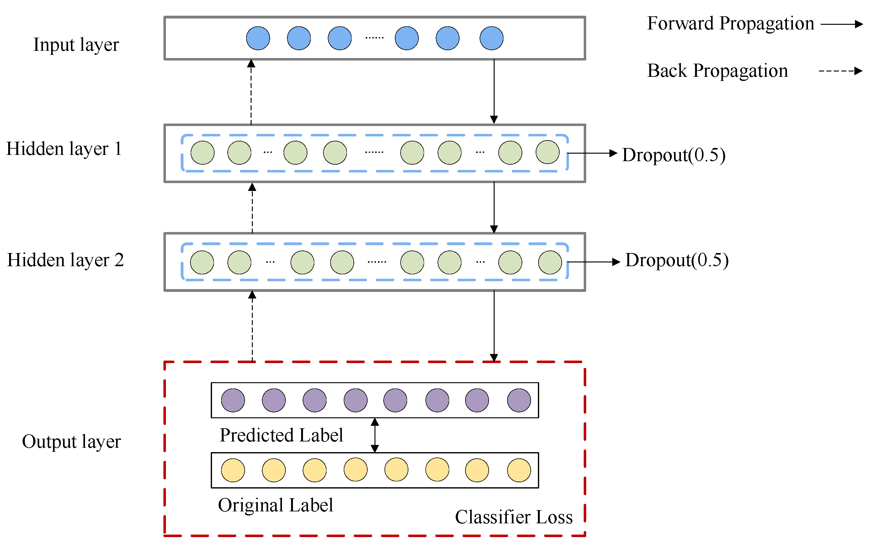
The 936 samples that have been processed were divided and 50% of the sample set was used as a training set to train the classifier, 30% of the sample set was used as the test set, to test the classification result, and 20% of the sample set was used as a validation set. The constructed neural network framework is shown in Figure 4.

For generally simple data sets, one or two hidden layers are usually sufficient [23]. Besides, the model with 2 hidden layers can represent an arbitrary decision boundary to arbitrary accuracy with rational activation functions [24]. Thus, we applied a neural network with two hidden layers. As for the number of neurons in the hidden layer, it often relies on trial-by-error to adjust in actual application. After several attempts, we determined the number of neurons in the hidden layer.

The learning curve of the BP neural network is shown in Figure 5. It can be seen from the figure that there is no over-fitting or under-fitting in the model. Moreover, the classifier shows good overall accuracy.

The main aim of this study is to identify the fault location from the fault phenomena recorded in natural language through the NN (Neural Network) classifier, which is a multi-classification problem. In general, a confusion matrix is used to assess the classification performance of the classifier. In the confusion matrix, the predicted labels of samples are compared to their original labels to show whether they are correctly classified.

The confusion matrix showing the diagnostic accuracy of the model is shown in Figure 6. As can be seen from the figure, the diagnostic accuracy of both the BTM and VCU fault components is relatively low. The other types of fault components achieve better diagnostic accuracy.

The generalizability of the classifier is evaluated based on the confusion matrix. Widely used metrics include:

$$Recall=\frac{TP}{TP+FN}$$

(14)

$$Precision=\frac{TP}{TP+FP}$$

(15)

$$f1-measure=\frac{2\times precision\times recall}{precision+recall}$$

(16)

where: TN: True Negative, TP: True Positive, FN: False Negative, and the recall statistic indicates the accuracy of correct classification of a certain type. Precision indicates the accuracy of the classification result. The f1 measure is a comprehensive evaluation index given by recall and precision; when the f1 value is high, the experimental model is ideal.

The performance metrics for evaluating the generalization performance of the classifiers based on the confusion matrix are shown in

Table 4. The performance metrics of the BP neural network.

Fault Components	Precision	Recall	f1-Score
BTM	0.60	0.91	0.72
DMI	0.89	0.86	0.88
GSM-R	1.00	0.97	0.99
JRU	0.94	1.00	0.97
SDU	0.97	0.97	0.97
TCR	0.91	0.97	0.94
TIE	0.83	0.58	0.68
VCU	0.71	0.74	0.72
Average	0.86	0.86	0.86

.

7.2. Naive Bayesian Model

Since the Naive Bayesian model is one of the most widely used classification models and the Naive Bayesian model is also widely used in fault diagnosis fields, we use Naive Bayesian for the final step, and the results will be compared with the BP neural network to prove the superiority of our proposed method. Because the Naive Bayesian model is only used as a comparison item, it will not state the principle of the model too much, but only show the classification results of the model.

Figure 7 shows the Naive Bayesian network structure derived from data. The confusion matrix showing the classification results and the performance metrics of the Naive Bayesian model is shown in Figure 8 and

Table 5. The performance metrics of the naive Bayesian model.

Fault Components	Precision	Recall	f1-Score
BTM	0.28	1	0.18
DMI	0.89	0.23	0.11
GSM-R	1.00	0.90	0.85
JRU	1.00	0.98	0.97
SDU	1.00	0.43	0.31
TCR	0.97	0.95	0.88
TIE	0.54	0.21	0.04
VCU	0.73	0.78	0.43
Average	0.80	0.68	0.47

.

As is shown in Table 5, the precision value of some key components, like BTM and VCU, is low, which means the prediction result is unreliable.

7.3. Comparison of Results

From the results, it can be concluded that:

(1) The method we propose is feasible. From the perspective of prediction accuracy and the average value of the three indicators (precision, recall, and f1-score), the prediction effect of the BP neural network is far better than that of naive Bayesian, which further confirms the reliability of the method we have proposed.

(2) Both classification models have a high probability of correctly classifying BTM faults (recall), which are 0.91 and 1 respectively. However, the precision values of both models are small. The precision value obtained by the BP neural network is 0.6, while the value obtained by the naive Bayesian model is 0.28, which further proves the superiority of the BP neural network performance and the relative reliability of classification results.

(3) The recall values of the TIE fault obtained by the two classification models are small, which means the possibility of a TIE fault is correctly classified is low. The recall value obtained by the BP neural network is 0.58, while the value obtained by the naive Bayesian model is 0.21. However, the precision value obtained by the BP neural network is very high, reaching 0.83. In other words, the prediction results for TIE faults obtained by the BP neural network are highly reliable.

(4) The recall and precision values of the DMI, GSM-R, JRU, SDU, TCR, and VCU faults obtained by the BP neural network are more balanced, and the prediction performance for these faults is ideal.

(5) The average values for the precision, recall, and f1-score of all fault components obtained by the BP neural network are 0.86, 0.86, and 0.86, respectively. While, the values obtained by the naive Bayesian model are 0.80, 0.68, and 0.47. Based on the results shown above, we can draw a conclusion that the model we proposed may be considered for fault analysis and diagnosis.

8. Conclusions

We have proposed a solution for sustainable fault diagnosis in the CTCS on-board equipment, based on imbalanced text mining. The reason why the method we proposed is sustainable is that this trained model can be used in other CTCS-3 fault data sets with good accuracy and facilitate the development of operation and maintenance work. In addition, when more data can be collected in the future, the model will be continuously trained by more data to further improve accuracy, which is also a manifestation of sustainability. The fault diagnosis problem is formulated as a classification problem. First, the fault data described in natural language is preprocessed, the fault features extracted, and the feature thesaurus is created. Next, the feature words are extracted from the fault data according to the feature thesaurus using TF-IDF and converted into vectors. Following this step, due to the imbalance of the fault dataset, the borderline-SMOTE algorithm is used to generate synthetic minority samples to avoid the negative effect of imbalance on classification performance. Finally, the fault data are classified using a BP neural network to determine the fault components. The results show that the overall performance of the classifier is relatively stable compared with the naive Bayesian model, and the average values of precision, recall, and f1-score are 0.86, 0.86, and 0.86 respectively. Therefore, the model can be used for fault diagnosis analysis.

There are several plausible directions for future research. First, we will collect more data and add more samples to the database to cover more failure types. Second, we will refine the cause of the fault using sufficient data to locate the fault specifically. The ultimate goal is to realize an intelligent fault diagnosis method for the CTCS on-board equipment, improve the maintenance efficiency of the high-speed railway signaling system, and ensure the safety of train operations. During the period of the new coronavirus epidemic, higher requirements are put forward for the automatic management of train operations. The fault diagnosis method can effectively support the automatic operation of urban rail transit.

References

- Shangguan, W.; Zhang, J.; Feng, J.; Cai, B. Fault diagnosis method of the on-board equipment of train control system based on rough set theory. J. China Railw. Soc. 2017, 40, 1–6. [Google Scholar]
- Zuo, Z.; Wang, K.; Wei, Y.; Zhao, X. Wireless connection timeout fault diagnosis of Chinese train control system using adaptive neuro-fuzzy inference system. In Proceedings of the 2017 Chinese Automation Congress (CAC), Jinan, China, 20–22 October 2017. [Google Scholar]
- Liu, J.; Cai, B.; Wang, J. A fault detection and diagnosis method for Speed Distance Units of high-speed train control systems. In Proceedings of the 2016 35th Chinese Control Conference (CCC), Chengdu, China, 27–29 July 2016; pp. 10258–10263. [Google Scholar] [CrossRef]
- Zhao, J.; Zheng, W. Study of fault diagnosis method based on fuzzy Bayesian network and application in CTCS-3 train control system. In Proceedings of the 2013 IEEE International Conference on Intelligent Rail Transportation Proceedings, Beijing, China, 30 August–1 September 2013; pp. 249–254. [Google Scholar] [CrossRef]
- Liang, X.; Wang, H.F.; Guo, J. Bayesian network based fault diagnosis method for on-board equipment of train control system. J. China Railw. Soc. 2017, 39, 93–100. [Google Scholar]
- Cheng, Y.; Xu, T.; Yang, L. Bayesian network based fault diagnosis and maintenance for high-speed train control systems. In Proceedings of the 2013 International Conference on Quality, Reliability, Risk, Maintenance, and Safety Engineering (QR2MSE2013), Emeishan, China, 15–18 July 2013; pp. 1753–1757. [Google Scholar]
- Bin, C.; Baigen, C.; Wei, S. Text mining in fault analysis for on-board equipment of high-speed train control system. In Proceedings of the 2017 Chinese Automation Congress (CAC), Jinan, China, 20–22 October 2017; pp. 6907–6911. [Google Scholar]
- Wang, F.; Xu, T.; Tang, T.; Zhou, M.; Wang, H. Bilevel Feature Extraction-Based Text Mining for Fault Diagnosis of Railway Systems. IEEE Trans. Intell. Transp. Syst. 2017, 18, 49–58. [Google Scholar] [CrossRef]
- Kang, Q.; Chen, X.; Li, S.; Zhou, M. A Noise-Filtered Under-Sampling Scheme for Imbalanced Classification. IEEE Trans. Cybern. 2017, 47, 4263–4274. [Google Scholar] [CrossRef] [PubMed]
- Kang, Q.; Shi, L.; Zhou, M.; Wang, X.; Wu, Q.; Wei, Z. A Distance-Based Weighted Undersampling Scheme for Support Vector Machines and its Application to Imbalanced Classification. IEEE Trans. Neural Netw. Learn. Syst. 2018, 29, 4152–4165. [Google Scholar] [CrossRef] [PubMed]
- Lala, H.; Karmakar, S. Detection and Experimental Validation of High Impedance Arc Fault in Distribution System Using Empirical Mode Decomposition. IEEE Syst. J. 2020, 14, 3494–3505. [Google Scholar] [CrossRef]
- Kou, L.; Liu, C.; Cai, G.-W.; Zhang, Z.; Zhou, J.-N.; Wang, X.-M. Fault diagnosis for three-phase PWM rectifier based on deep feedforward network with transient synthetic features. ISA Trans. 2020, 101, 399–407. [Google Scholar] [CrossRef] [PubMed]
- Yang, X.; Yang, C.; Yang, C.; Peng, T.; Chen, Z.; Wu, Z.; Gui, W. Transient fault diagnosis for traction control system based on optimal fractional-order method. ISA Trans. 2020, 102, 365–375. [Google Scholar] [CrossRef] [PubMed]
- Kou, L.; Liu, C.; Cai, G.; Zhou, J.; Yuan, Q.; Pang, S. Fault diagnosis for open-circuit faults in NPC inverter based on knowledge-driven and data-driven approaches. IET Power Electron. 2020, 13, 1236–1245. [Google Scholar] [CrossRef]
- Hu, Z.-X.; Wang, Y.; Ge, M.-F.; Liu, J. Data-Driven Fault Diagnosis Method Based on Compressed Sensing and Improved Multiscale Network. IEEE Trans. Ind. Electron. 2019, 67, 3216–3225. [Google Scholar] [CrossRef]
- Cabrera, D.; Guamán, A.; Zhang, S.; Cerrada, M.; Sánchez, R.-V.; Cevallos, J.; Long, J.; Li, C. Bayesian approach and time series dimensionality reduction to LSTM-based model-building for fault diagnosis of a reciprocating compressor. Neurocomputing 2020, 380, 51–66. [Google Scholar] [CrossRef]
- Zhou, T.; Wang, Y.; Wang, C.-X.; Salous, S.; Liu, L.; Tao, C. Multi-Feature Fusion Based Recognition and Relevance Analysis of Propagation Scenes for High-Speed Railway Channels. IEEE Trans. Veh. Technol. 2020, 69, 8107–8118. [Google Scholar] [CrossRef]
- Wei, L.; Qian, Z.; Zareipour, H. Wind Turbine Pitch System Condition Monitoring and Fault Detection Based on Optimized Relevance Vector Machine Regression. IEEE Trans. Sustain. Energy 2020, 11, 2326–2336. [Google Scholar] [CrossRef]
- Zhong, K.; Han, M.; Han, B. Data-driven based fault prognosis for industrial systems: A concise overview. IEEE/CAA J. Autom. Sin. 2020, 7, 330–345. [Google Scholar] [CrossRef]
- Han, H.; Wang, W.Y.; Mao, B.H. Borderline-SMOTE: A new over-sampling method in imbalanced data sets learning. In Advances in Intelligent Computing, Proceedings of the International Conference on Intelligent Computing, ICIC 2005, HeFei, China, 23–26 August 2005; Part I; Springer: Berlin/Heidelberg, Germany, 2005; pp. 878–887. [Google Scholar]
- Chawla, N.V.; Bowyer, K.W.; Hall, L.O.; Kegelmeyer, W.P. SMOTE: Synthetic minority over-sampling technique. J. Artif. Intell. Res. 2002, 16, 321–357. [Google Scholar] [CrossRef]
- Srivastava, N.; Hinton, G.; Krizhevsky, A.; Sutskever, I.; Salakhutdinov, R. Dropout: A Simple Way to Prevent Neural Networks from Overfitting. J. Mach. Learn. Res. 2014, 15, 1929–1958. [Google Scholar]
- Reed, R.; Marks, R.J., II. Neural Smithing—Supervised Learning in Feedforward Artificial Neural Networks. Pattern Anal. Appl. 2001, 4, 73–74. [Google Scholar]
- Lecun, Y.; Bengio, Y.; Hinton, G. Deep Learning. Nature 2015, 521, 436–444. [Google Scholar] [CrossRef] [PubMed]