Article

Feasibility of Different Weather Data Sources Applied to Building Indoor Temperature Estimation Using LSTM Neural Networks

by
Martín Pensado-Mariño
1,*,
Lara Febrero-Garrido
2,
Pablo Eguía-Oller
1 and
Enrique Granada-Álvarez
1
1
GTE Research Group, Department of Mechanical Engineering, Heat Engines and Fluids Mechanics, Industrial Engineering School, University of Vigo, Maxwell, s/n, 36310 Vigo, Spain
2
Defense University Center, Spanish Naval Academy, Plaza de España s/n, 36920 Marín, Spain
*
Author to whom correspondence should be addressed.
Sustainability 2021, 13(24), 13735; https://doi.org/10.3390/su132413735
Submission received: 25 October 2021 / Revised: 3 December 2021 / Accepted: 5 December 2021 / Published: 13 December 2021
(This article belongs to the Topic Sustainable Smart Cities and Smart Villages)

Abstract

:
The use of Machine Learning models is becoming increasingly widespread to assess energy performance of a building. In these models, the accuracy of the results depends largely on outdoor conditions. However, getting these data on-site is not always feasible. This article compares the temperature results obtained for an LSTM neural network model, using four types of meteorological data sources. The first is the monitoring carried out in the building; the second is a meteorological station near the site of the building; the third is a table of meteorological data obtained through a kriging process and the fourth is a dataset obtained using GFS. The results are analyzed using the CV(RSME) and NMBE indices. Based on these indices, in the four series, a CV(RSME) slightly higher than 3% is obtained, while the NMBE is below 1%, so it can be deduced that the sources used are interchangeable.

1. Introduction

In the coming decades, the number of inhabitants of large cities will continue to rise to around 70% by 2050, according to United Nations (UN) information [1]. For the European Union (EU), the building sector represents an energy expenditure of approximately 40% of the energy produced [2]. In the case of the United States (US), this percentage increases to about 50% [3]. This energy is mainly used in heating, ventilation and air conditioning (HVAC) systems [4]. Managing adequately the energy used in these systems will lead to a reduction in emissions and consumption.
This growth will entail the challenge of making more efficient buildings to have sustainable cities. The application of energy simulation technologies like EnergyPlus or TRNSyS has been generalised in the last few years [5,6,7]. These tools make it possible to carry out sensitivity analyses that result in a better utilization of energy. Nevertheless, the construction of this model requires detailed knowledge about the system and, in spite of it, may present a gap in the actual building due to uncertainties and inaccuracies in the construction [8]. In this context, the application of Artificial Intelligence (AI) provides a reliable alternative in terms of speed and accuracy [9]. There is a wide variety of applications, overall using Machine Learning and Deep Learning algorithms, where these models have proved their effectiveness learning complex patterns and modelling non-linear relationships [10,11,12]. As a disadvantage, these models require a large amount of data about the system they are modelling.
A very widespread application of Machine Learning in the field of energy efficiency in which these models have proven their effectiveness is in the modelling of the thermal comfort conditions [13] and the control of the installations [14,15]. Attoue et al. [16], using a recurrent structure based on an MLP (Multilayer perceptron) Neural Network were capable of reaching a coefficient of correlation (R) above 0.8 for a 4-h horizon. They also highlight the existing time-dependency inherent in the system. This time dependency requires a neural network called Recurrent Neural Network (RNN). These networks allow information from previous steps to persist, so that this memory is taken into account to obtain the next time step. Xu et al. [17] compared the performance of three Machine Learning models and two Deep Learning models and concluded that LSTM models have advantages over the rest of he forecasting models, showing a slight increase of the R 2 value. Long Short-Term Memory (LSTM) neural networks are a type of RNN developed by Hochreiter [18] to solve the disappearance gradient problem, by allowing gradients flow unchanged. However, LSTM networks can still suffer the explosive gradient problem. Other authors increased the precision of LSTM models using Convolutional layers (CNN) [19] and adaptive hyperparameter configurations [20].
A point in common for all models is the utilization of weather data. Weather conditions have a great influence on the prediction of internal conditions. The implantation of Internet of things (IoT) in buildings, to collect information about the indoor conditions and facilities behaviour, may contribute to reducing the gap between the energy model and the real building. This technology is applicable to both new and existing buildings, with different strategies for monitoring it depending on the objectives [21,22]. However, in the case of outdoor conditions its applicability is less. The measurement of meteorological conditions has more restrictive requirements. Traditionally, Typical Meteorological Years (TMY) [23] have been used, based on statistics. Currently, the availability of other data sources takes time leading TMY to disuse and increasing the utilization of more accurate options. The most appropriate strategy to pursue would be gathering in-site measurements. However, the measurement of weather conditions requires the installation of expensive equipment that must fulfil certain technical criteria that cannot always be reached. In this case, the simplest way is to use data collected by a nearby weather station. However, there is not always some near the emplacement, besides that, the further away it is from the building the less the accuracy will be. To mitigate this problem, interpolation between several stations can be a solution. Interpolation techniques, such as Thin Plate Spline (TPS) [24] and Nearest Neighbour (NN) [25], amend the lack of precision caused by the position of the weather station. An interpolation technique that has been well received to tackle problems like this is kriging, with various examples on this field [26,27]. Another inconvenience that comes with the use of weather stations is that often the data are not public, which limits their use. In this context, the option of using Numerical Weather Prediction (NWP) models with open access outputs like Global Forecast System (GFS) or Global Data Assimilation System (GDAS) arises. More information about GFS and GDAS physics can be found in [28]. This source differs from the previous sources in that the data will no longer come from a measurement but is a weather forecast.
The intention of this work is to develop a comparative framework for different sources of meteorological data. For this purpose, the LSTM Neural Network will be fed with the data of the building under study together with the meteorological conditions from different sources. These sources will be analysed to detect the possible weaknesses of each method. By obtaining the metrics of Coefficient of Variation of the Root Mean Square Error (CV(RMSE)), Normalized Mean Bias Error (NMBE) y R 2 is intended to evaluate the accuracy and strengths of each of them.

2. Materials and Methods
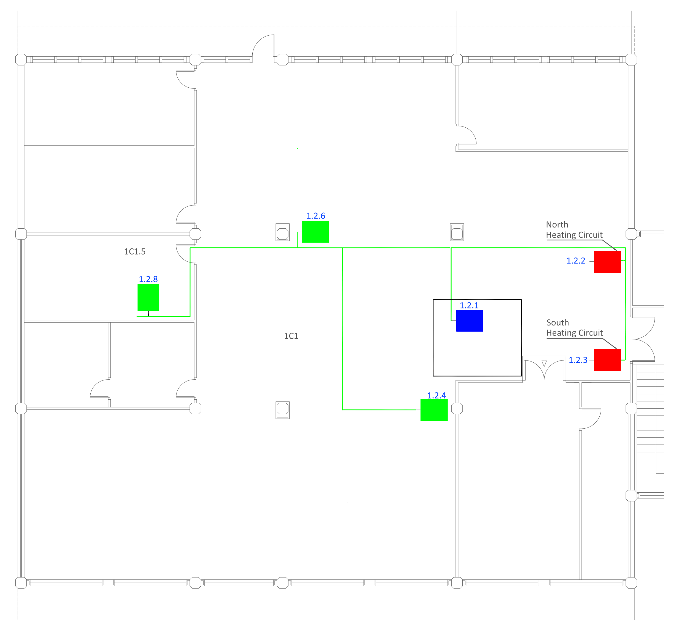
2.1. Building Data

The building under study is the Rectorate of the University of the Basque Country (UPV/EHU), located in the north of Spain. This building, which is used as an office building, is divided into three blocks (west, center and east) composed of four floors. This work is centered on the first floor of the west block (Figure 1). The building was retrofitted in 2017 and monitors the indoor conditions and the consumption of thermal and electrical installations. First floor sensors can be divided into three groups: in Figure 1, the group of sensors that measure indoor conditions (temperature, relative humidity and CO 2 in parts per million) are marked in green, and the blue and red squares indicate the electrical and thermal consumption sensors, respectively. Data are used in hourly frequency.
The variables for which more than one sensor is mounted are used as a single composite series with the average values.

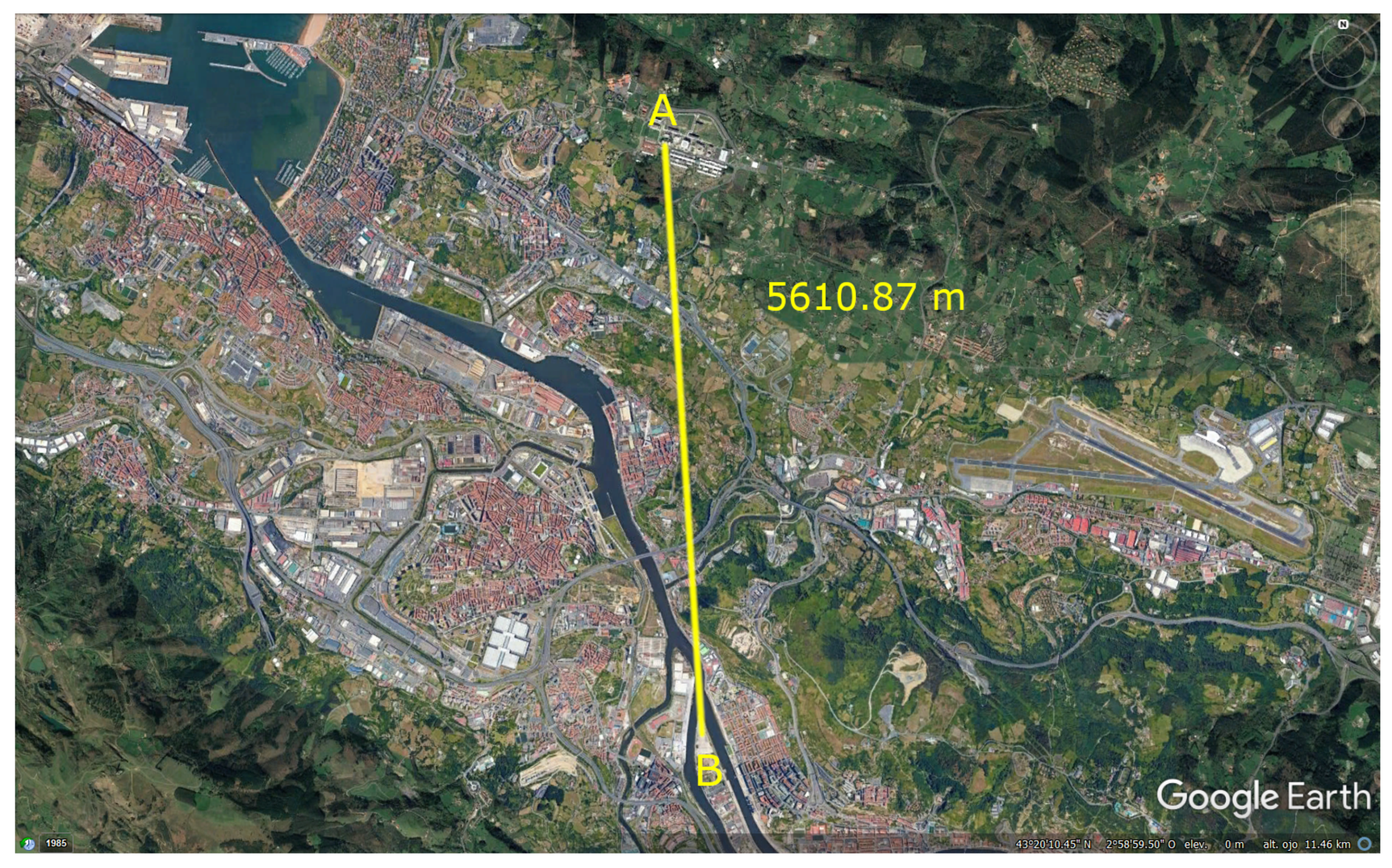
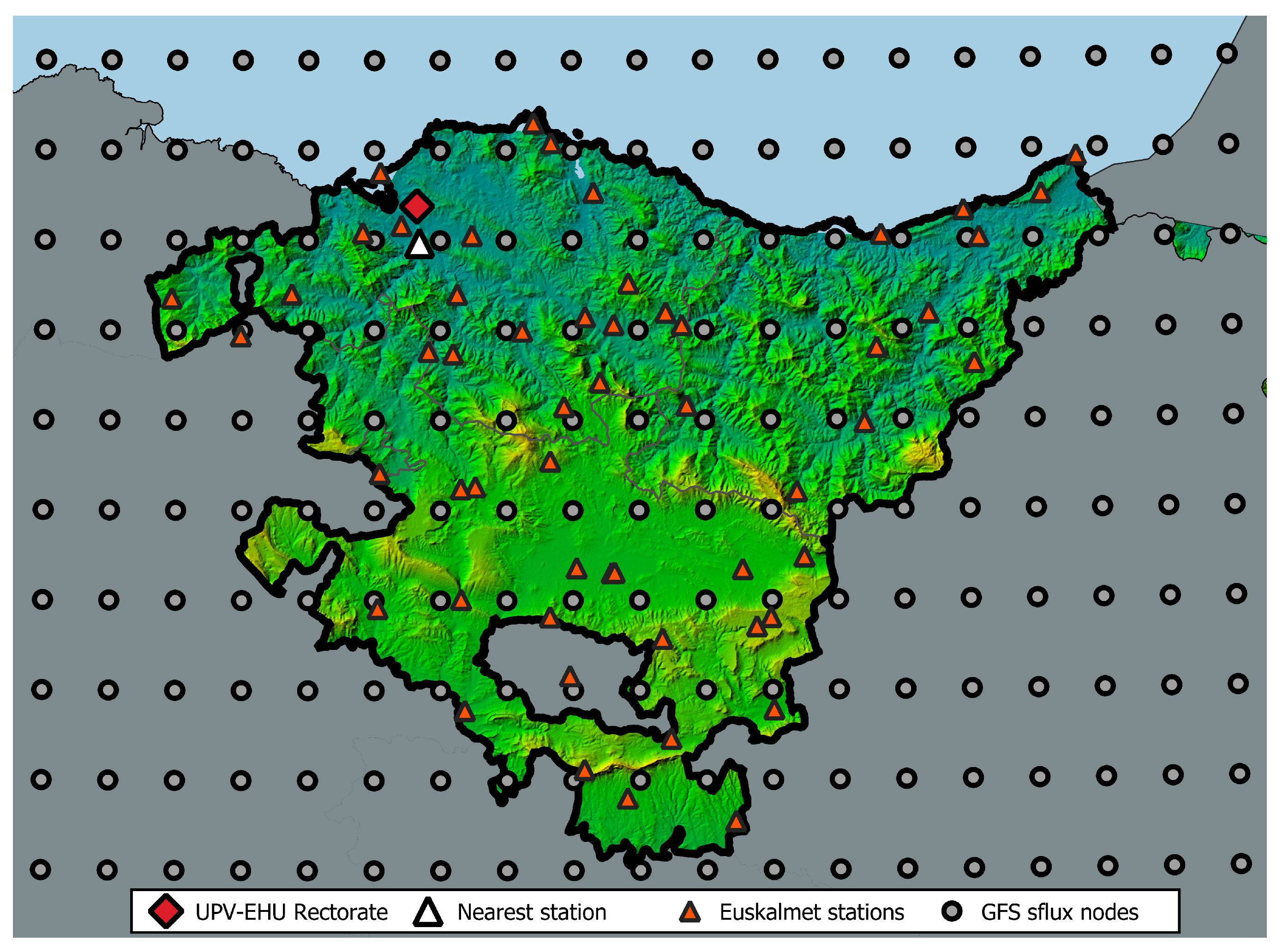
2.2. Meteorological Data

Meteorological data are obtained from four sources, two of which are based on measurements, while the other two are based on mathematical models.
The first source based on measurements is the building itself (building series), which has mounted a set of sensors on the roof to measure the weather conditions of temperature, wind speed, rain (yes or no), relative humidity, solar irradiance, and luminosity, but only temperature, relative humidity and solar irradiance have been considered. These data are obtained with a ten-minute frequency.
The second source of meteorological data is the weather station C039-Deusto (43.283407 N, −2.966659 W Altitude 3 m). This station belongs to the Euskal Meteorologia Agentzia (Euskalmet) network and is located about 5.6 km in a straight line from the building under study, as shown in Figure 2. It is the closest station to the building that measures the variables described above. As with the previous source, only temperature, relative humidity and solar irradiance are taken into account.
The third source of meteorological data is a kriging interpolation applied over the entire network of Euskalmet weather stations. The family of kriging methods is named after the geology and mining work of Krige [29], further developed by Matheron [30]. The kriging process is based on the principle that the properties of the points closest to the target are more similar to that of the furthest points.
For a generic variable Z(x) to be interpolated, this spatial correlation means that it can be decomposed by two components: a deterministic part m(x), which expresses large-scale variations of Z(x), and a random part A(x), which accounts for small-scale variations due to uncertainties and measurement errors. Equation (1) shows this decomposition:
Z ( x ) = m ( x ) + A ( x ) .
All kriging processes are based on this principle. In this study, the kriging version—called Universal Kriging—is applied, which uses additional variables (in this case latitude, longitude, elevation and land-sea proximity) that model the spatial tendency at the global scale of the main variable.
Figure 3 shows the network of weather stations (black) and the location of the Rectorate building.
The fourth data source is the Global Forecast System (GFS) model, a numerical weather prediction model developed by the National Oceanic and Atmospheric Administration (NOAA) of the US. This model uses scattered weather observations from different sources to generate meteorological forecasts over a regular grid that covers all the planet. The GFS surface flux (GFS sflux) product, which is the particular implementation of GFS used here, has a spatial horizontal resolution of about 13 km at the equator. The mesh resolution is represented in Figure 3.
It provides 1-h resolution forecasts four times each day (at 00, 06, 12 and 18 h UTC), covering a range of several days for each forecast execution. The grid nodes of GFS sflux covering the Basque Country are shown in Figure 4. The meteorological variables extracted from the GFS sflux forecast files are temperature at 2 m height, relative humidity, and short wave downwards solar irradiation.
This model provides 1-h resolution forecasts four times each day (at 00, 06, 12 and 18 h UTC), covering a range of several days for each forecast execution. The grid nodes of GFS sflux covering the Basque Country are shown in Figure 3. The meteorological variables extracted from the GFS sflux forecast files are temperature at 2 m height, relative humidity, and short wave downwards solar irradiation.
The Figure 3 illustrates the different sources of meteorological data:
The location of the Rectorate building is indicated by the red rhombus. The corner triangles represent each of the meteorological stations that compose the Euskalmet network, and located to the south of the building and highlighted by the white triangle is the nearest station. The grey circles symbolize each of the GFS nodes, although the node east of the nearest station is the one used in this case.

2.3. LSTM Neural Networks

The LSTM neural network is a variety of recurrent neural network the architecture of which is designed for modelling time sequences and their upstream dependencies.
The operation of LSTM cells is determined by their internal structure, consisting of three doors: input, forget and output. The forget gate takes the input value and the previous hidden state and decides which information is relevant and which is missing from it. The input gate updates the value of the cell with new information. The output gate determines the hidden state of the cell. Through this door structure, LSTM cells are able to retain relevant information.
The combination of conventional hidden layers and LSTM cells is the first step on the construction of the case architecture. These cells are combined using, in each case, the optimal configuration for the problem to be solved. Since it is intended to compare the results for four data sources, the same network will be used in all cases, so that the variation of the results is not influenced by the network architecture.
One of the most important parameters of LSTM networks is time-lag. Using this value, a certain amount of previous time steps are sent to the network. The decision to use three or 24 previous steps has a great influence on the results and depends on the characteristics of the building and the facilities of the same that are studied. In this case, a value of 12 h has been taken, based on previous work [31].
The literature on the configuration of a neural network is extensive and the possibilities are innumerable [32,33,34,35]; therefore, the search for this configuration is usually delimited to a grid. This tool establishes a series of intervals that define the parameters to be evaluated. In this work, the parameters for which the grid will be applied are the relationship layers LSTM—hidden layers, the number of neurons, the number of epochs, according to the limits collected in Table 1:
The parameters that will remain fixed are the optimizing algorithm, which is Adaptive Moment Estimation (Adam) [36]; the activation function, using the Rectified Linear Unit (ReLU) [37] and the batch size, equal to 64 [38]. The patience option is also used. This early stop option is used to prevent overfitting [39] from occurring and works by stopping the training loop in the event that a certain amount of the set epochs is reached and no improvement in the results has occurred [40]. Since epochs are a variable parameter, 20% is set as a limit.

2.4. Pre-Processing Data

LSTM neural networks work with a continuous data series. The sample used is composed of observations from 1 January 2018 to 31 May 2019. The entirety of 2018 is used to train the model, while 2019 breaks down into the 5 months available and will be used as training or as a test according to the month. That is, to obtain February 2019, January 2019 would be part of training. From the variables monitored in the building, those collected in Figure 5 are used in the model.
In addition to the variables coming from the monitoring, variables referring to the date will be used to provide more information to the network. In particular, the variables “Hour of the day”, “Day of the week”, “Month of the year” and “Day of the year” are created. A categorical variable to express the season was also included.
The variables describing building conditions are obtained with an hourly frequency, so the meteorological variables, which are obtained in a ten minute frequency, have been resampled using the mean value to coincide with the building variables. Both types of variables can contain empty spaces or outliers. This type of discontinuity can add noise to the network and affect the quality of the results, due to the continuous character of LSTM neural networks.
These values have been filtered to eliminate outliers caused by sensor errors (p.e. relative humidity is known to be between 0% and 100%) and converted into missing values. This filtering can increase the number of missing values. As indicated, LSTM networks use continuous values, so to reduce the amount of missing data, these gaps are subsequently filled by second order polynomial interpolation, setting as a condition of application the number of consecutive values equal to or less than three. If this condition is not met, interpolation does not apply. Values that do not meet this condition will be masked through a scaling before being introduced into the neural network.

2.5. Validation and Error Measurement

To measure the forecasting technique’s performance, the Normalized Mean Biased Error (NMBE) and the Coefficient of Variation of the Root Mean Squared Error (CV(RMSE)) are used. NMBE is commonly used to detect whether the model is producing an underestimation (NMBE > 0) or an overestimation (NMBE < 0) and its magnitude (Equation (2)).
N M B E = 100 · i = 1 N ( M i S i ) M ¯ .
In Equation (2), N is the number of samples, S i is the forecasting value, M i is the observation value and M ¯ is the mean value of the observations.
On the other hand, CV(RMSE) is the RMSE, normalized by the mean of the observation values. It is used as a primary measure of error to assess the quality of the models created (Equation (3)).
C V ( R M S E ) = 100 · 1 M ¯ i = 1 N ( M i S i ) 2 N .
In Equation (3), the variables used are the same as in Equation (2). Following the criteria established by the ASHRAE on Guideline 14 [41], for hourly forecasting, a CV(RMSE) lower than 30% allows us to consider the model as calibrated.
In addition to these two indicators, the coefficient of determination ( R 2 ) has been used. This coefficient, obtained by Equation (4), indicates how close simulated values are to the regression line of the measured values [42]. Its value is between 0 and 1, a value close to 1 meaning a good fit between the simulated and measured values.
R 2 = n · i = 1 N ( M i S i ) i = 1 N ( M i ) · i = 1 N ( S i ) ( n · i = 1 N M i 2 ( i = 1 N M i ) 2 ) · ( n · i = 1 N S i 2 ( i = 1 N S i ) 2 ) ) 2 .
For this indicator, the ASHRAE Guideline [41] and the International Performance Measurement and Verification Protocol (IPVMP) [43] recommend a value greater than 0.75 in calibrated models.

3. Results and Discussion

3.1. Meteo Data Analysis

Differences between the four meteorological data sources employed need to be understood and analysed. To do this, two different concepts are observed: amount and distribution of missing values and difference with real observations. This analysis is applied to the dataset once preprocessed. In Figure 6 the three variables of each of the four meteorological data sources are represented. Lighter areas represent the missing data.
Attention is also paid to the number of missing values in each source, a fact that can greatly influence the results due to the discontinuities in the series of data used by the LSTM network. To prevent attributes in larger numerical ranges from dominating those in smaller numerical ranges all variables are scaled and, since missing values cannot be deleted due to the fact that LSTM neural networks work with continuous data, missing values are masked. In this case, data are scaled between 0 and 1 and a missing value is represented with −1.
It can be observed how the data obtained in-situ are those that present a greater amount of missing data, especially in the irradiation series, which presents 21.98% of missing values. In the case of the Euskalmet meteorological station, the percentage is very low, 0.87% of all data. In the case of kriging data, only the missing irradiation data are relevant, in the case of 5.51%. While for data obtained by meteorological stations, missing data may be due to a sensor failure, for the GFS it is due to a download failure on the server. In this case, the series preserves a total of 102 missing data corresponding to August 2018, so it is estimated that its influence will be low by not making estimates for any summer month of 2019.
To compare the four datasets, we took as a reference the data from the measurements in the building and studied the difference with the other sources. These differences are plotted on the x-axis histogram in Figure 7, where the y-axis indicates the frequency of occurrence. We can observe the distance of the Euskalmet, Kriging and GFS tables with respect to the measurements obtained in the building. This does not imply that the building measurements are correct, since the sensors are subject to measurement errors.
The temperatures histogram shows how Euskalmet and Kriging series are more centered, that is, these series are more similar to those of the building. On the other hand, the GFS series is advanced, which means that the temperature values are below the measurements of the building. A similar situation happens for relative humidity. In addition, in this case, the Euskalmet series is closer to that of the building. For Kriging series, data are placed at an intermediate point between the GFS and Euskalmet. Globally, the three series are more distant than in the case of temperature. Taking into account the solar irradiation, differences dispersion is much higher than the two other variables, although the three series present at least 4% of the values in the range [−10, 10]. As with relative humidity, the series are very far from the established reference, although in this case it should be noted that the irradiation series presents the greatest amount of missing data, which have not been represented.
Figure 7 does not represent all the differences obtained, since the queues in the chart showed a very low percentage (≤1%). The Table 2 shows the percentage of values not represented in the graph.
Jointly analysing Figure 7 and the values contained in Table 2, it can be deduced that the temperature presents a much greater proximity than the series of relative humidity and solar irradiation.

3.2. Indoor Temperature Analysis

This section compares the results of indoor temperature predictions for different meteorological data sources. The prediction sample covers from 1 January 2018 to 31 May 2019, separated into five cuts and using the same neural network configuration. Figure 8 shows three arbitrary samples 5 days long.
It can be seen how the predictions follow the trend of the measurements although with differences. For January and March, colder months where the influence of heating is greater than the influence of solar irradiation, the prediction is closer to the actual curve. For the month of May, when the days are warmer, predictions are below the real curve, meaning that the network gives less importance to irradiation than to heat consumption. As predictions were realized for the same floor, this factor is considered to have no influence on the results and therefore only climatic differences have an effect. Missing values for 2019 are only present for irradiation on Building and Kriging series but seeing the results, this does not seem to have much influence. Based on Figure 8, it is not possible to determinate which outcome of the predictions best fits the measured values, making error analysis necessary.

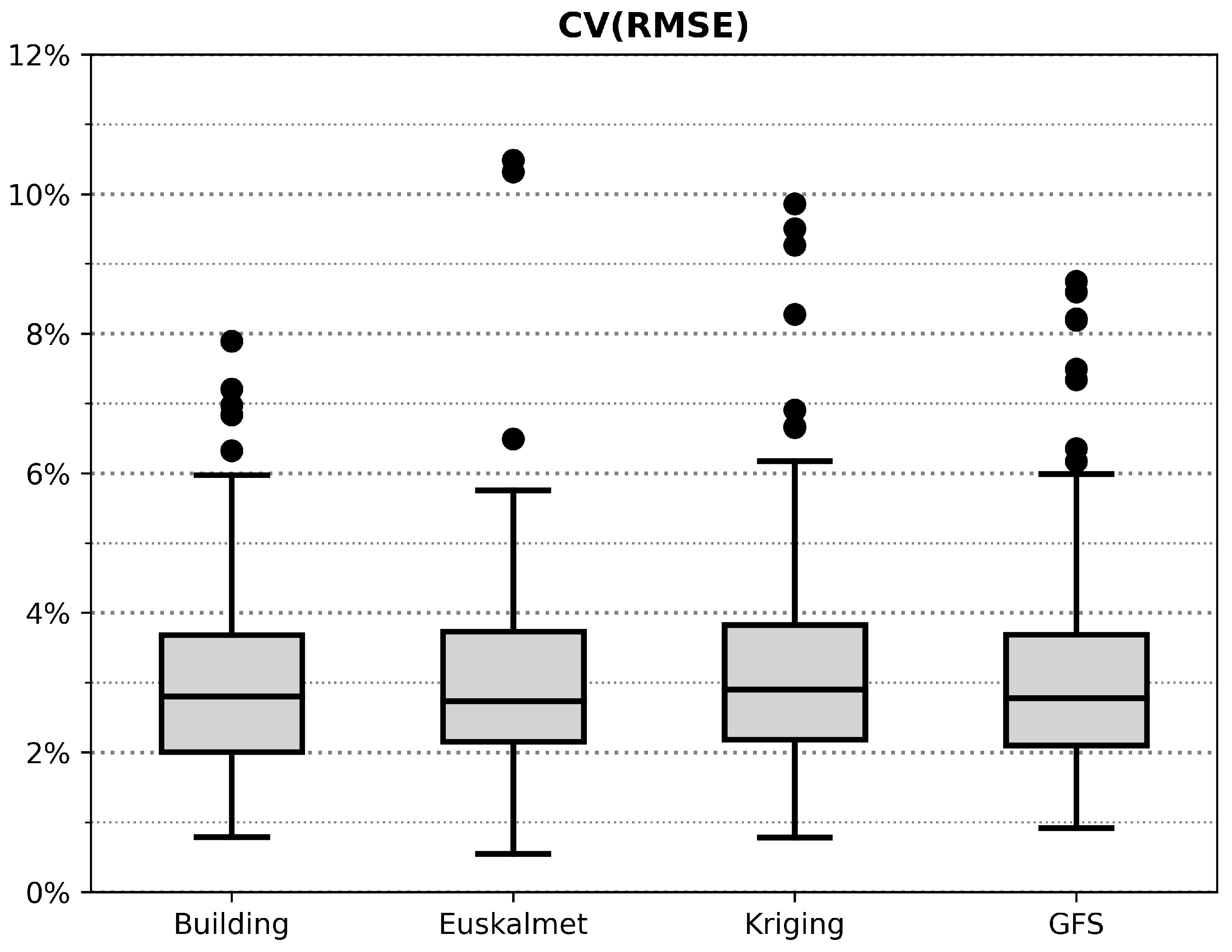
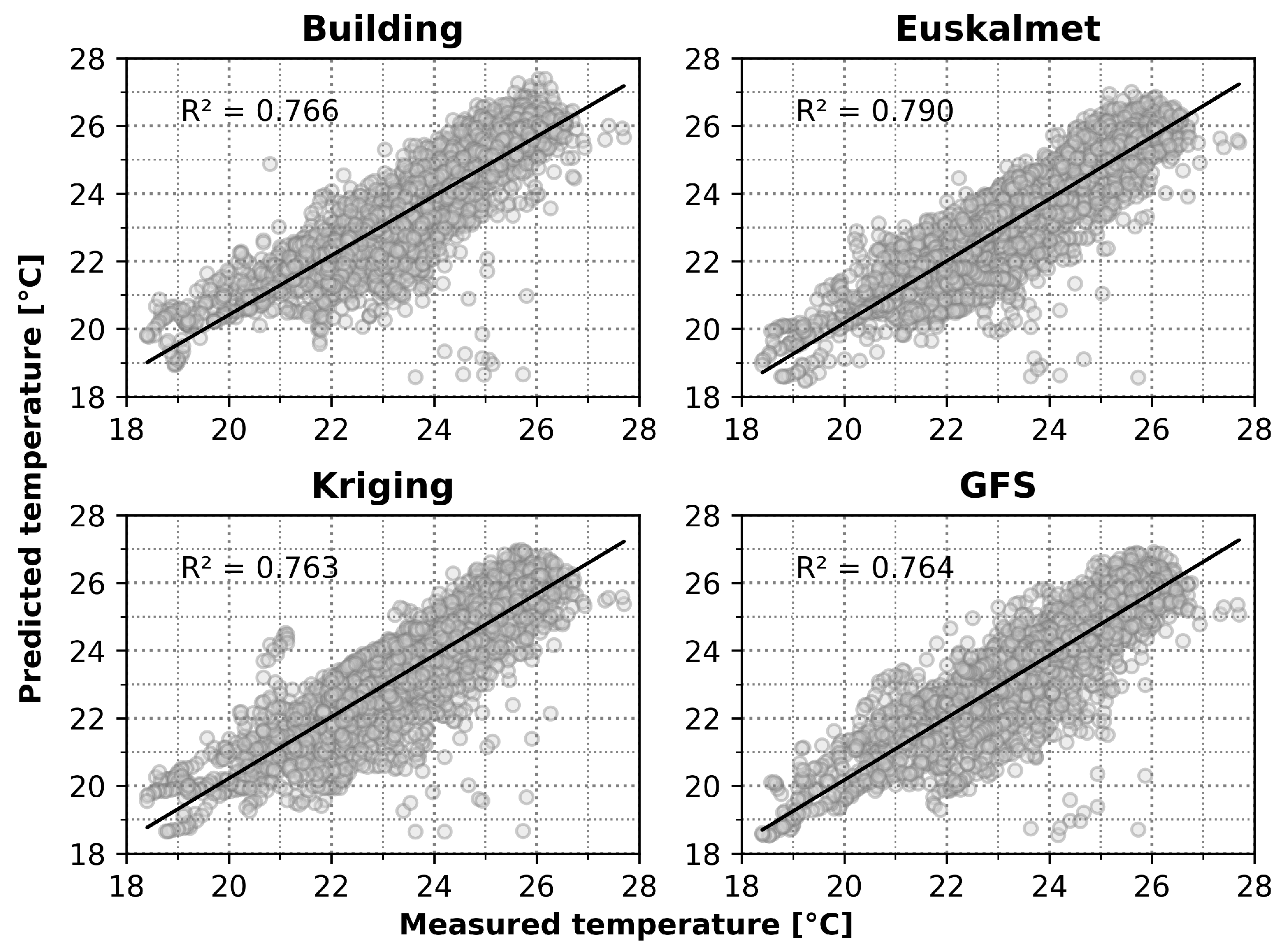
3.3. Error Measurement and Performance Analysis

To analyze the performance of each of the data sources when making accurate predictions of the interior temperature of the first floor, the indicators are explained in Section 2.5.
Figure 9 illustrates CV(RMSE), calculated for the entire period of each meteorological data series. It can be seen that the median of all samples is similar; however, the Building series shows the most centered range.
The interquartile range of the four sources is in all cases below 2%, which implies a stable and bounded error. In the case of moustaches, the four series have a range of close to 5%, although it is the GFS series that has a lower range. It is worth noting the presence of outliers in all the series, although with different relevance, Euskalmet being the one that presents a smaller quantity of outliers while in the Building they are below 8%, being the only series in which it occurs.
To further quantify these errors, Table 3 is added, which includes the CV(RMSE) for each month, as well as the total of each series.
This values show that all predictions are around a CV(RMSE) close to 3%. If we detail the analysis to the observation for months, it is notable that February and May show the smallest error, while April contains the biggest error of all series, although the results for these periods do not differ greatly from the trend observed for the other months
If we analyzed each series of data, the errors point to a better behaviour of the Euskalmet and Building results. This can be explained by the accuracy of the Building data and the continuity of the Euskalmet data. By changing the focus, looking at Figure 7, the similarity between the Euskalmet series with the Building series is on the line with the results obtained. In turn, although the GFS series is more distant from the measurements inside the building than the Kriging series, this one has a higher percentage of missing values, while the GFS series is lower in terms of magnitude.
On the other hand, to represent the NMBE results, Figure 10 is used. It represents each of the series facing the average indoor temperature and the predictions obtained. This also includes the adjustment of the results, expressed by the index R 2 :
The R 2 value shows how the four series are slightly above 0.75, with the Euskalmet series showing the higher value and the kriging series showing the lowest value, but very close to Building and GFS. These results are similar to those obtained for CV (RMSE). The series present certain values with a great deviation from the general trend, although there is no one that stands out in this aspect. Several of these values can be observed in similar positions for the different series, especially in values below the R 2 value, so they are likely to be caused by missing values in the common data. The results of the calculation of the NMBE are shown in Table 4:
The negative values present in the first three months mean that, in those months, the model produces an overestimation, while in the rest of the cases an underestimation is produced. Due to these differences, the value of the overall adjustment of each series is very close to zero, it being remarkable that the phenomenon of overestimation is present only in global value of the Building series, which in turn is the closest to zero.
Comparing the values of Table 4 with Figure 8, the concordance between the NMBE values and the behaviour of the series with respect to the values measured by the internal sensors can be assessed.
Summarizing the conclusions drawn from each analysis, it can be assumed that the results are within the margins established, referred to in the ASHRAE Guideline 14 [41] and the IPVMP [43], in order to consider them appropriate. In addition, there is no series that stands out as remarkable above the others in the results. There are differences between each series and also between the different months; however, both the overall values and the results of each month do not point to a series with clearly differentiated results.

4. Conclusions

As seen in Section 3.3 Error Measurement and Performance Analysis, the total errors are within 3% for the CV(RMSE) and in the lower range of +−0.5% for the NMBE for all four sources. If we compare the value of R 2 differences between the series and previous results, such as those obtained by Xu et al. [17], we see that R 2 is slightly below their results, being around 0.89 for the network with a time step of 5 min and 0.79 for a time step of 30 min. For the case of Elmaz et al. [19], the use of a CNN layer allows them to reach values of 0.911 for a time step of 60 min, corresponding to the one used in this work.
If we compare R 2 values, the differences between the Building, Kriging and GFS series are in the order of thousandths. The fact of obtaining this result emphasizes the problem of missing data, being that the Building series presents a greater amount of them, as shown in Figure 6. In the case of Kriging, although the amount of missing data is much lower, this result could also have influenced this result. The case of the GFS data is remarkable, since they are essentially predictive data, instead of real measurements, as is the case for the rest of the data sources. If we look at Figure 7, it can be seen how the GFS series is the one that is farthest away from the in-building measurements. Nevertheless, the LSTM network has been able to adapt to this difference in magnitudes. The fact of obtaining errors in the order of the rest of the series may be useful for future predictions. Moreover, being a global source, it can be applied to any part of the world using the same treatment and acquisition process. The use of such data would make it possible to anticipate energy consumption and therefore optimize the use of sources. Considering the results of Euskalmet, and despite coming from a weather station far from the building, the proximity of the data to those of the building and the practical absence of missing data have allowed us to obtain an adjustment in R 2 superior by 3% to the rest of the sources.
In short, the results obtained show that the three alternative sources of meteorological data analysed (Euskalmet, Kriging and GFS) allow indoor temperature models to be generated for buildings of adequate quality and accuracy. The results for these predictive models are comparable to those obtained using intensive (and invasive) monitoring of the building interior. This leads to the conclusion that the use of such alternative, free and non-invasive data sources has great potential for application in building energy efficiency modelling and prediction studies.
The feasibility of using alternative data sources for the in-site measurement of meteorological conditions at a building site is therefore concluded. The proposed sources are varied, which means that for the same case there may be more than one possibility. This becomes relevant given the influence of this information on the model results.
On the other hand, it opens the door to the use of GFS data for the prediction of building conditions such as future estimates of heat consumption or other relevant energy variables. Knowledge of this information could enable optimization of the energy production and storage process, a key step in the construction and design of more efficient and sustainable buildings and facilities.

Author Contributions

Conceptualization, P.E.-O. and M.P.-M.; methodology, M.P.-M. and P.E.-O.; software, M.P.-M.; validation, L.F.-G., E.G.-Á.; formal analysis, M.P.-M., L.F.-G.; investigation, M.P.-M.; resources, E.G.-Á.; data curation, L.F.-G.; writing, original draft preparation, M.P.-M. and L.F.-G.; writing, review and editing, M.P.-M., P.E.-O. and L.F.-G.; visualization, M.P.-M. and P.E.-O.; supervision, P.E.-O. and E.G.-Á.; project administration, P.E.-O. and E.G.-Á.; funding acquisition, P.E.-O. and E.G.-Á. All authors have read and agreed to the published version of the manuscript.

Funding

This research was supported by the Ministry of Science, Innovation and Universities of Spanish Government under the SMARTHERM project (RTI2018-096296-B-C2).

Institutional Review Board Statement

Not applicable.

Informed Consent Statement

Not applicable.

Data Availability Statement

Not applicable.

Conflicts of Interest

The authors declare no conflict of interest.

References

  1. United Nations, Department of Economic and Social Affairs. 2018 Revision of World Urbanization Prospects; United Nations, Department of Economic and Social Affairs: 2019. Available online: https://population.un.org/wup/Publications/Files/WUP2018-Report.pdf (accessed on 1 December 2021).
  2. European Commission, Department of Energy. Energy Efficiency in Buildings; European Commission, Department of Energy: 2020. Available online: https://ec.europa.eu/info/news/focus-energy-efficiency-buildings-2020-feb-17_en (accessed on 1 December 2021).
  3. U.S. Energy Information Administration. U.S. Energy Consumption by Source and Sector 2020; U.S. Energy Information Administration, 2020. Available online: https://www.eia.gov/energyexplained/us-energy-facts/ (accessed on 1 December 2021).
  4. International Energy Agency. Buildings Energy Efficiency 2020 Analysis; International Energy Agency: 2020. Available online: https://iea.blob.core.windows.net/assets/59268647-0b70-4e7b-9f78-269e5ee93f26/Energy_Efficiency_2020.pdf (accessed on 1 December 2021).
  5. Martínez-Mariño, S.; Eguía-Oller, P.; Granada-Álvarez, E.; Erkoreka-González, A. Simulation and validation of indoor temperatures and relative humidity in multi-zone buildings under occupancy conditions using multi-objective calibration. Build. Environ. 2021, 200, 107973. [Google Scholar] [CrossRef]
  6. Roberti, F.; Oberegger, U.; Gasparella, A. Calibrating historic building energy models to hourly indoor air and surface temperatures: Methodology and case study. Energy Build. 2015, 108, 236–243. [Google Scholar] [CrossRef] [Green Version]
  7. Bughio, M.; Khan, M.; Mahar, W.; Schuetze, T. Impact of passive energy efficiency measures on cooling energy demand in an architectural campus building in karachi, pakistan. Sustainability 2021, 13, 7251. [Google Scholar] [CrossRef]
  8. Martínez, S.; Eguía, P.; Granada, E.; Moazami, A.; Hamdy, M. A performance comparison of multi-objective optimization-based approaches for calibrating white-box building energy models. Energy Build. 2020, 216, 109942. [Google Scholar] [CrossRef]
  9. MacCarana, Y.; Panza, A.; Maroni, G.; Sarto, L.; Carta, M.; Reggiani, S. Comparison of model-based and data-driven approaches for modeling energy and comfort management systems, with a case study. In Proceedings of the 2019 IEEE International Conference on Environment and Electrical Engineering and 2019 IEEE Industrial and Commercial Power Systems Europe (EEEIC/I&CPS Europe), Genova, Italy, 11–14 June 2019. [Google Scholar] [CrossRef]
  10. Neto, A.; Fiorelli, F. Comparison between detailed model simulation and artificial neural network for forecasting building energy consumption. Energy Build. 2008, 40, 2169–2176. [Google Scholar] [CrossRef]
  11. Hung, N.; Babel, M.; Weesakul, S.; Tripathi, N. An artificial neural network model for rainfall forecasting in Bangkok, Thailand. Hydrol. Earth Syst. Sci. 2009, 13, 1413–1425. [Google Scholar] [CrossRef] [Green Version]
  12. Guresen, E.; Kayakutlu, G.; Daim, T. Using artificial neural network models in stock market index prediction. Expert Syst. Appl. 2011, 38, 10389–10397. [Google Scholar] [CrossRef]
  13. Martínez-Comesaña, M.; Ogando-Martínez, A.; Troncoso-Pastoriza, F.; López-Gómez, J.; Febrero-Garrido, L.; Granada-Álvarez, E. Use of optimised MLP neural networks for spatiotemporal estimation of indoor environmental conditions of existing buildings. Build. Environ. 2021, 205, 108243. [Google Scholar] [CrossRef]
  14. Kathirgamanathan, A.; De Rosa, M.; Mangina, E.; Finn, D. Data-driven predictive control for unlocking building energy flexibility: A review. Renew. Sustain. Energy Rev. 2021, 135, 110120. [Google Scholar] [CrossRef]
  15. Cordeiro-Costas, M.; Villanueva, D.; Eguía-Oller, P. Optimization of the electrical demand of an existing building with storage management through machine learning techniques. Appl. Sci. 2021, 11, 7991. [Google Scholar] [CrossRef]
  16. Attoue, N.; Shahrour, I.; Younes, R. Smart building: Use of the artificial neural network approach for indoor temperature forecasting. Energies 2018, 11, 395. [Google Scholar] [CrossRef] [Green Version]
  17. Xu, C.; Chen, H.; Wang, J.; Guo, Y.; Yuan, Y. Improving prediction performance for indoor temperature in public buildings based on a novel deep learning method. Build. Environ. 2019, 148, 128–135. [Google Scholar] [CrossRef]
  18. Hochreiter, S.; Schmidhuber, J. Long Short-Term Memory. Neural Comput. 1997, 9, 1735–1780. [Google Scholar] [CrossRef]
  19. Elmaz, F.; Eyckerman, R.; Casteels, W.; Latré, S.; Hellinckx, P. CNN-LSTM architecture for predictive indoor temperature modeling. Build. Environ. 2021, 206, 108327. [Google Scholar] [CrossRef]
  20. Luo, X.; Oyedele, L. Forecasting building energy consumption: Adaptive long-short term memory neural networks driven by genetic algorithm. Adv. Eng. Inform. 2021, 50, 101357. [Google Scholar] [CrossRef]
  21. Imran; Ahmad, S.; Kim, D. Design and implementation of thermal comfort system based on tasks allocation mechanism in smart homes. Sustainability 2019, 11, 5849. [Google Scholar] [CrossRef] [Green Version]
  22. Hitimana, E.; Bajpai, G.; Musabe, R.; Sibomana, L.; Kayalvizhi, J. Implementation of iot framework with data analysis using deep learning methods for occupancy prediction in a building. Futur. Internet 2021, 13, 67. [Google Scholar] [CrossRef]
  23. Chan, A.; Chow, T.; Fong, S.; Lin, J. Generation of a typical meteorological year for Hong Kong. Energy Convers. Manag. 2006, 47, 87–96. [Google Scholar] [CrossRef]
  24. Suparta, W.; Rahman, R. Spatial interpolation of GPS PWV and meteorological variables over the west coast of Peninsular Malaysia during 2013 Klang Valley Flash Flood. Atmos. Res. 2016, 168, 205–219. [Google Scholar] [CrossRef]
  25. López Gómez, J.; Troncoso Pastoriza, F.; Fariña, E.; Eguía Oller, P.; Granada Álvarez, E. Use of a numerical weather prediction model as a meteorological source for the estimation of heating demand in building thermal simulations. Sustain. Cities Soc. 2020, 62, 102403. [Google Scholar] [CrossRef]
  26. Dalmau, R.; Pérez-Batlle, M.; Prats, X. Estimation and prediction of weather variables from surveillance data using spatio-temporal Kriging. In Proceedings of the 2017 IEEE/AIAA 36th Digital Avionics Systems Conference (DASC), St. Petersburg, FL, USA, 17–21 September 2017. [Google Scholar] [CrossRef] [Green Version]
  27. Kuo, P.F.; Huang, T.E.; Putra, I. Comparing kriging estimators using weather station data and local greenhouse sensors. Sensors 2021, 21, 1853. [Google Scholar] [CrossRef] [PubMed]
  28. National Oceanic and Atmospheric Administration. NOAA, NCEP Products Inventory. 2010. Available online: https://www.nco.ncep.noaa.gov/pmb/products/gfs/ (accessed on 1 December 2021).
  29. Krige, D. A statistical approach to some basic mine valuation problems on the Witwatersrand. J. Chem. Metall. Min. Soc. Afr. 1951, 52, 119–139. [Google Scholar]
  30. Matheron, G. Principles of geostatistics. Econ. Geol. 1963, 58, 1246–1266. [Google Scholar] [CrossRef]
  31. Pensado-Mariño, M.; Febrero-Garrido, L.; Pérez-Iribarren, E.; Oller, P.; Granada-álvarez, E. Estimation of heat loss coefficient and thermal demands of in-use building by capturing thermal inertia using lstm neural networks. Energies 2021, 14, 5188. [Google Scholar] [CrossRef]
  32. Sheela, K.; Deepa, S. Review on methods to fix number of hidden neurons in neural networks. Math. Probl. Eng. 2013, 2013, 425740. [Google Scholar] [CrossRef] [Green Version]
  33. Tej, M.; Holban, S. Determining Optimal Neural Network Architecture Using Regression Methods. In Proceedings of the 2018 International Conference on Development and Application Systems (DAS), Suceava, Romania, 24–26 May 2018; pp. 180–189. [Google Scholar] [CrossRef]
  34. Sheela, K.; Deepa, S. Selection of number of hidden neurons in neural networks in renewable energy systems. J. Sci. Ind. Res. 2014, 73, 686–688. [Google Scholar]
  35. Madhiarasan, M.; Deepa, S. A novel criterion to select hidden neuron numbers in improved back propagation networks for wind speed forecasting. Appl. Intell. 2016, 44, 878–893. [Google Scholar] [CrossRef]
  36. Bock, S.; Weis, M. A Proof of Local Convergence for the Adam Optimizer. In Proceedings of the 2019 International Joint Conference on Neural Networks, IJCNN 2019, Budapest, Hungary, 14–19 July 2019. [Google Scholar] [CrossRef]
  37. Eckle, K.; Schmidt-Hieber, J. A comparison of deep networks with ReLU activation function and linear spline-type methods. Neural Netw. 2019, 110, 232–242. [Google Scholar] [CrossRef]
  38. Li, M.; Zhang, T.; Chen, Y.; Smola, A.J. Efficient mini-batch training for stochastic optimization. In Proceedings of the 20th ACM SIGKDD International Conference on Knowledge Discovery and Data Mining, New York, NY, USA, 24–27 August 2014; pp. 661–670. [Google Scholar] [CrossRef]
  39. Bilbao, I.; Bilbao, J. Overfitting problem and the over-training in the era of data: Particularly for Artificial Neural Networks. In Proceedings of the 2017 Eighth International Conference on Intelligent Computing and Information Systems (ICICIS), Cairo, Egypt, 5–7 December 2017; pp. 173–177. [Google Scholar] [CrossRef]
  40. Gulli, A.; Pal, S. Deep Learning with Keras; Packt Publishing Ltd.: Birmingham, UK, 2017. [Google Scholar]
  41. ASHRAE. Guideline 14–2014—Measurement of Energy, Demand, and Water Savings; ASHRAE: Atlanta, GA, USA, 2014. [Google Scholar]
  42. Ruiz, G.; Bandera, C. Validation of calibrated energy models: Common errors. Energies 2017, 10, 1587. [Google Scholar] [CrossRef] [Green Version]
  43. Efficiency Valuation Organization. International Performance Measurement and Verification Protocol: Concepts and Options for Determining Energy and Water Savings; Efficiency Valuation Organization, 2012. Available online: https://www.nrel.gov/docs/fy02osti/31505.pdf (accessed on 1 December 2021).
Figure 1. Location of the sets of sensors installed on the First Floor.
Sustainability 13 13735 g001
Figure 2. Distance between the Rectorate building (A) and the nearest weather station (B). Source: “Bilbo” 43°17′11.56″ N and 2°58′50.59″ O. Google Earth. 23 March 2021. 10 October 2021.
Sustainability 13 13735 g002
Figure 3. Map of the Basque country showing all meteorological data sources used.
Sustainability 13 13735 g003
Figure 4. LSTM recurrent neural network architecture.
Sustainability 13 13735 g004
Figure 5. Monitored variables included in the model.
Sustainability 13 13735 g005
Figure 6. Meteorological series gaps plot.
Sustainability 13 13735 g006
Figure 7. Difference between building’s weather station measurements and the measurements of the rest of the sources.
Sustainability 13 13735 g007
Figure 8. Results of temperature predictions.
Sustainability 13 13735 g008
Figure 9. Boxplot of the CV(RMSE) results for the first floor.
Sustainability 13 13735 g009
Figure 10. Results dispersion with R2 value.
Sustainability 13 13735 g010
Table 1. Neural network tuned hyperparameters.
ParameterLower LimitUpper LimitIncrease
LSTM-Hidden layers3-25-41-1
Number of neurons5020050
Number of epochs100300100
Table 2. Percentage of non plotted data differences.
TemperatureRelative HumidityIrradiation
Euskalmet0.17%0.59%0.67%
Kriging0.25%0.86%0.48%
GFS0.22%1.00%0.89%
Table 3. Error values comparison of the CV(RMSE).
JanuaryFebruaryMarchAprilMayTotal
Building3.14%2.87%3.12%3.30%2.76%3.04%
Euskalmet3.16%2.87%3.06%3.44%2.60%3.02%
Kriging3.32%2.71%3.74%3.42%2.74%3.19%
GFS2.80%2.59%3.50%3.98%2.76%3.13%
Table 4. Error values comparison of the NMBE.
JanuaryFebruaryMarchAprilMayTotal
Building−1.85%−1.00%−0.62%1.89%0.96%−0.10%
Euskalmet−0.50%−0.51%0.34%2.03%0.74%0.45%
Kriging−0.33%0.06%−0.42%1.74%0.48%0.31%
GFS−0.87%−0.68%−0.36%2.95%0.58%0.35%
Publisher’s Note: MDPI stays neutral with regard to jurisdictional claims in published maps and institutional affiliations.

