Marginal Abatement Cost of Carbon Emissions under Different Shared Socioeconomic Pathways

Abstract

Future emissions scenarios have served as a primary basis for assessing climate change and formulating climate policies. To explore the impact of uncertainty in future emissions scenarios on major outcomes related to climate change, this study examines the marginal abatement cost (MAC) of carbon emissions under the latest Shared Socioeconomic Pathways (SSPs) subject to the economic optimum and the 1.5 °C temperature increase constraint using the Epstein-Zin (EZ) climate model. Taking the “Regional Rivalry” (SSP3) scenario narrative under the economic optimum as a representative case, the expected MACs per ton CO₂ equivalent (CO₂e) emissions in the years 2015, 2030, 2060, 2100, and 2200 are: $102.08, $84.42, $61.19, $10.71, and $0.12, respectively. In parallel, the associated expected average mitigation rates (AMRs) are 0%, 63%, 66%, 81%, and 96%, respectively. In summary, in a world developing towards regional rivalry (SSP3) or fossil-fueled development (SSP5) with high mitigation pressure, the MAC values have approximately doubled, compared with the sustainability (SSP1) and inequality (SSP4) storylines with low mitigation pressure levels. The SSP2 (Middle of the Road) shows a moderate MAC decreasing trend with moderate mitigation pressure. The results provide a carbon price benchmark for policy makers with different attitudes towards the unknown future and can be used to formulate carbon mitigation strategy to respond to specific climate goals.

1. Introduction

Since the start of industrialization, economic development and population growth have driven the high use of carbon-based fossil fuels. This has been followed by a steady increase in atmospheric carbon emissions and higher carbon concentrations, and has triggered global climate change. In response, an increasing number of countries have proposed carbon trading and carbon tax policies to effectively encourage emission reduction. Both approaches place a price on carbon dioxide (CO₂) emission permits and enable economic entities to reduce CO₂ emissions. Marginal cost theory proposes that, in a perfectly competitive market, the optimal price per unit of CO₂ emission permit should be equal to the marginal abatement cost (MAC), defined as the cost to reduce one unit of CO₂ emissions at a specific emission level [1]. Therefore, measuring the MAC of CO₂ can provide a carbon price benchmark.

The interactions between climate change and economic development are highly uncertain. As such, quantitatively analyzing optimal abatement costs under uncertainty requires a recursive dynamic programming implementation of Integrated Assessment Models (IAMs) [2]. IAMs modelers use several generations of emission scenarios to develop a series of impact assessments with respect to climate change [3]. In other words, emission scenario storylines provide input drivers to climate models, and climate models output major variables of climate change. These variables are of direct interest to policymakers concerned about the design of mitigation policies, such as emissions, concentrations, temperature, MACs, mitigation rates, and the social cost of carbon (SCC) [4].

Emission scenarios describe what the future could look like and provide several possible futures [5]. The climate change community has developed several generations of emissions scenarios. These include the “1990 IPCC First Scientific Assessment” (SA90) [6], the “1992 IPCC Scenarios” (IS92) [7], the 2000 IPCC “Special Report on Emission Scenarios” (SRES) [8], and the 2010 “Representative Concentration Paths” (RCPs) [9] and the 2017 “Shared Socio-economic Pathways (SSPs)” [10] developed outside the IPCC. Currently, SSPs are starting to be used in climate modeling and were prepared for the IPCC sixth assessment report.

Many studies have discussed future climate change mitigation, adaptation, and broader social and environment sustainability issues under the framework of SSPs scenarios. Chen et al. applied a 14-region global TIMES model (GTIMES) to study mid-to-long term energy development and carbon emission strategies for different regions using SSPs [11]. Bauer et al. explored future energy sector developments across the five SSPs, using five leading IAMs [12]. Yang et al. applied the GTIMES with scenarios designed using SSPs and RCPs, and created a detailed depiction of the quantification of SSP trajectories into the GTIMES model [13]. Yang et al. updated the SCC under the SSPs using the Dynamic Integrated Model of Climate and the Economy (DICE) [14]. Chen et al. projected future urban land expansions at a 1 km resolution at a global scale under SSPs using the FLUS model, and explored the potential impacts on the environment and food production [15].

SSPs have been successfully applied in different impact assessment studies; however, this coverage has not included predicting future MACs. This paper estimates the MACs under the SSP storylines by applying the Epstein-Zin (EZ) climate model; the associated average mitigation rates (AMRs) are given in parallel. We also compared the MACs under different SSPs. The key added value over previous studies is the impact of uncertainty in SSP narrative storylines on the MACs of carbon emissions. The MAC values provide a carbon price benchmark, and the AMR values provide a basis for formulating carbon mitigation strategies to assist policy makers with different approaches with respect to an unknown future.

This paper is organized as follows. Section 2 presents the SSP data set used for our analysis. Section 3 introduces the theoretical model, which includes the Epstein-Zin (EZ) recursive utility function, geophysical equation, emission reduction cost function, and climate damage function. Section 4 presents the simulation results. Focusing on the SSP3 narrative under the economically optimal policy as a representative case, this section presents the MACs and AMRs at five emission reduction decision timepoints for each state: 2015, 2030, 2060, 2100, and 2200. This section also presents the expected MACs and AMRs at the five emission reduction decision timepoints under the five SSPs. Then, the sensitivity of the main model parameters is analyzed. Section 5 concludes the paper.

2. Materials

The SSPs offer five scenario narratives, which describe broad socioeconomic trends that could shape different characteristics in a future society. All are baseline scenarios without future climate policies, i.e., the “business as usual” (BAU) scenarios. The five pathways include: SSP1 (Sustainability), SSP2 (Middle of the Road), SSP3 (Regional Rivalry), SSP4 (Inequality), and SSP5 (Fossil-fueled Development). Of them, SSP1 represents the green growth road. SSP2 involves a medium level of challenge associated with both mitigation and adaptation. SSP3 represents international fragmentation and regional rivalry. SSP4 considers the scenario of extreme inequality. SSP5 represents high levels of challenge with respect to mitigation and low challenges with respect to adaptation [10].

Climate scientists have examined how to adapt to different climate mitigation targets under five alternative pathways described by the SSPs for various outcomes in a future society. Similar to RCPs, climate mitigation targets are also defined by Radiative Forcing (RF), which is the net change (downward minus upward) radiative flux (expressed in $\mathrm{w}/{\mathrm{m}}^2$) at the tropopause or top of atmosphere due to a change in an external driver of climate change [16]. Climate mitigation targets are to limit RF within the time before 2100 to 8.5, 7.0, 6.0, 4.5, 3.4, 2.6, and 1.9 $\mathrm{w}/{\mathrm{m}}^2$, which are represented by RCP8.5, RCP7.0, RCP6.0, RCP4.5, RCP3.4, RCP2.6, and RCP1.9, respectively. Of these, RCP8.5 and RCP7.0 represent the “worst” and “average” no-policy scenarios, respectively. In this article, we use “RCPBaseline” to represent RCP8.5 or RCP7.0 scenarios. A total of 26 mitigation scenarios are constructed by combining mitigation targets of the RCPs with the five SSPs [17].

Table 1. All mitigation scenarios.

Shared Socioeconomic Pathways (SSPs)	Representative Concentration Paths (RCPs)	Mitigation Scenarios
SSP1 (Sustainability)	RCPBaseline	SSP1-Baseline
	RCP4.5	SSP1-4.5
	RCP3.4	SSP1-3.4
	RCP2.6	SSP1-2.6
	RCP1.9	SSP1-1.9
SSP2 (Middle of the Road)	RCPBaseline	SSP2-Baseline
	RCP6.0	SSP2-6.0
	RCP4.5	SSP2-4.5
	RCP3.4	SSP2-3.4
	RCP2.6	SSP2-2.6
	RCP1.9	SSP2-1.9
SSP3 (Regional Rivalry)	RCPBaseline	SSP3-Baseline
	RCP6.0	SSP3-6.0
	RCP4.5	SSP3-4.5
	RCP3.4	SSP3-3.4
SSP4 (Inequality)	RCPBaseline	SSP4-Baseline
	RCP6.0	SSP4-6.0
	RCP4.5	SSP4-4.5
	RCP3.4	SSP4-3.4
	RCP2.6	SSP4-2.6
SSP5 (Fossil-fueled Development)	RCPBaseline	SSP5-Baseline
	RCP6.0	SSP5-6.0
	RCP4.5	SSP5-4.5
	RCP3.4	SSP5-3.4
	RCP2.6	SSP5-2.6
	RCP1.9	SSP5-1.9

lists all mitigation scenarios.

Climate scientists have also described several different climate policies [18]. The first is a baseline policy, where no policies are taken to slow or reverse the greenhouse effect until 2250. The second policy is the “economic optimum” policy, where economically “optimal” policies are adopted to slow climate change. The third policy is a “CO₂ concentration constraints” policy, where CO₂ concentrations are constrained to a specific level. The fourth policy is a “temperature constraints” policy, where this century’s temperature increase is constrained to a specific level above pre-industrialization levels, usually at 1.5 or 2 °C. Nordhaus [18] noted that the “baseline policy” and “optimal policy” have fallen out of favor with analysts, who tend to focus on the temperature-limiting or concentration-limiting policies. However, the economically-focused “optimal policy” continues to have research value as a measure benchmark of efficiency or inefficiency when assessing other climate policies. Global efforts to mitigate climate change are guided by projections of future temperatures [19]. On 12 December 2015, parties to the UNFCCC (United Nations Framework Convention on Climate Change) reached the Paris Agreement, which established the goal of controlling global temperature increases to within 2 °C above the pre-industrial level, and pursuing a level below a 1.5 °C increase, during this century [20]. Therefore, we consider the scenarios where the economically optimal policy and the global temperature increase is kept within 1.5 °C pre-industrial levels in this century.

3. Theoretical Model

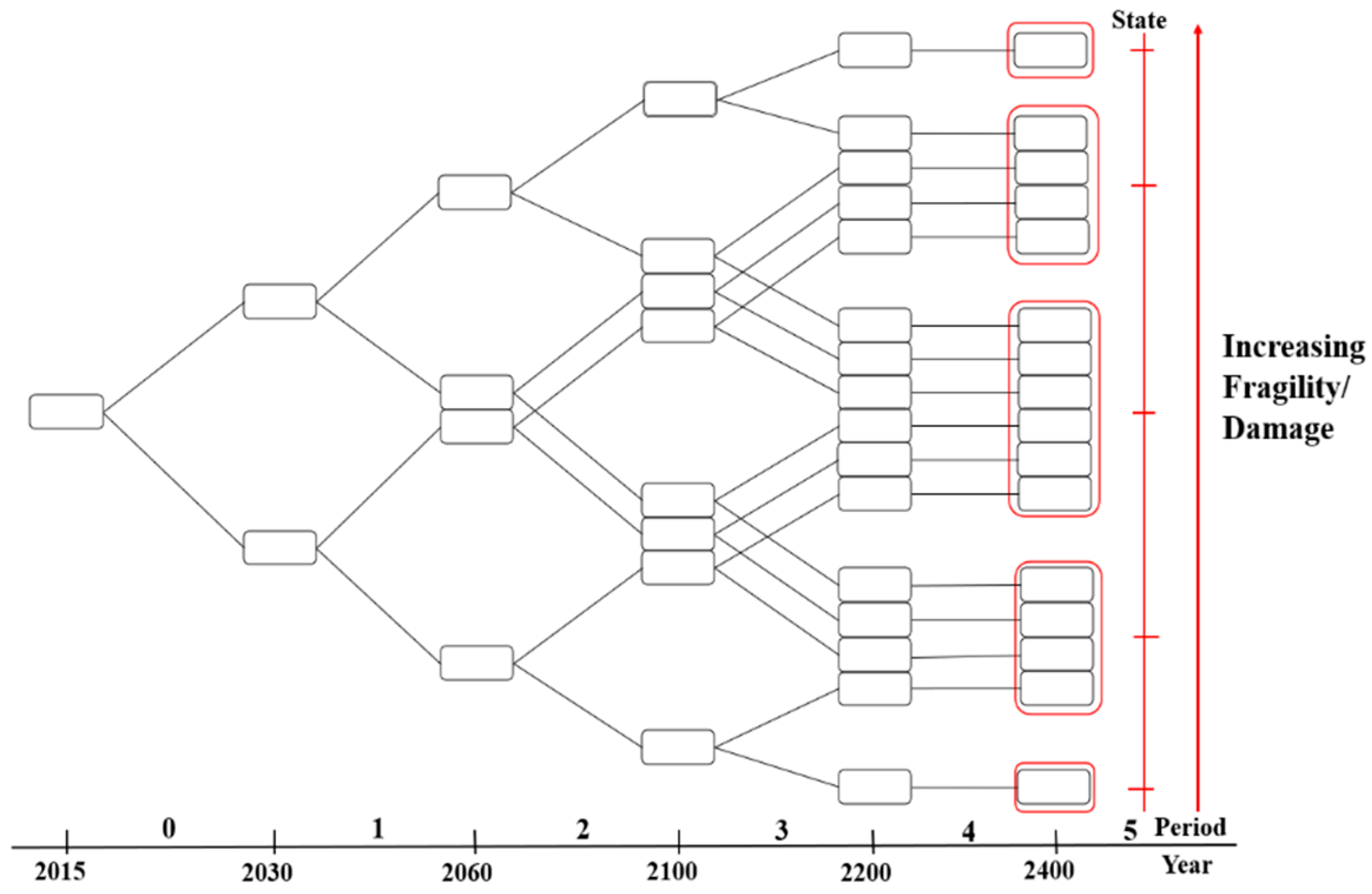
The studied time period is divided into 6 periods: (2015, 2030), (2030, 2060), (2060, 2100), (2100, 2200), (2200, 2400), and (2400, +∞). These correspond to period t = 0, 1, 2, 3, 4, and 5, with five-year time steps. There are five emission reduction decision time points: 2015, 2030, 2060, 2100, and 2200. Figure 1 shows the model tree structure. The connection line between two “boxes” indicates the path with information about ${\theta }_t$. The parameter ${\theta }_t$ is the climate fragility, which also represents all states of nature in period t. The five “red boxes” in 2400 represent the five states of nature, or nodes. The fragility or climate damage of each node in each period increases from the bottom to the top. At emission reduction decision time t, there are t + 1 states of nature, or nodes. Period 0 represents the time period from 2015 to 2030 with only one node. By 2030, there are two nodes to choose from and there is a 50% probability of each of the two nodes. Assume that, in an economy with a single representative agent, the representative agent knows in which state he is, an “up (u)” or “down (d)” state. Similarly, there are three nodes to choose from by 2060. Again, the representative agent knows whether the world is in the state of “uu”, “ud” (or “du”), or “dd”. At each state of nature in the binary tree, more information about ${\theta }_t$ and the resulting climate damage is revealed, before the uncertainty is fully resolved in 2200. Assuming that the representative agent takes no more actions to reduce carbon emissions from 2400 to infinity, a “2^T − 1” (T = 5) dimensional optimization problem is created as the essence of the model. Consumption grows deterministically after t = 2400 at a growth rate $r_0$. Therefore, consumption is defined as $C_t=C_T{\left(1+r_0\right)}^{\left(t-T\right)}$, when t > T. In the binary tree, all grouped or clustered nodes in a given period represent the same state, which has the same level of climate fragility. When the cumulative radiative forcing (CRF) is equal, the grouped or clustered nodes experience the same level of climate damage.

According to the framework of the EZ climate model, the Epstein-Zin recursive utility function, geophysical equation, abatement cost function, and climate damage function are all introduced. All prices are in 2015 international dollars for this study.

3.1. Epstein-Zin Recursive Utility Function

Daniel et al. [21] proposed that the Epstein-Zin recursive utility function of the representative agent in period t, t∈{0, 1, 2,…T}, is expressed as: $U_t={\left[\left(1-\beta \right)C_t^{\rho }+\beta {\left(E_t\left[U_{t+1}{}^{\alpha }\right]\right)}^{\frac{\rho }{\alpha }}\right]}^{\frac{1}{\rho }}$, where $E_t$ is the predicted value of period t + 1 based on the information of period t; $\delta$ is the time preference rate, $\delta =\left(1-\beta \right)/\beta$; $\sigma$ is the intertemporal substitution elasticity, $\sigma =1/(1-\rho )$; and $\mathsf{\eta }$ is the relative risk aversion coefficient, $\mathsf{\eta }=1-\alpha$.

The consumption of period t is expressed as:

$$\begin{gathered} C_0=\overline{C_0}\left[1-k_0\left(x_0\right)\right] C_t=\overline{C_t}\left[1-k_t\left(x_t\right)\right]\left[1-D_t\left(CR{F}_t,{\theta }_t\right)\right], \\ C_T=\overline{C_T}\left[1-D_T\left(CR{F}_T,{\theta }_T\right)\right] \end{gathered}$$

(1)

where the agent is endowed with a certain amount of the consumption good in period t, $\overline{C_t}$, $\overline{C_t}={\overline{C}}_0{\left(1+r_0\right)}^t$; and $r_0$ is the consumption growth rate. The climate damage function $D_t\left(CR{F}_t,{\theta }_t\right)$ captures the fraction of climate damage as a proportion of the endowed consumption. The CRF_t is the cumulative radiative forcing of atmospheric CO₂e emissions from period 0 to t, which determines the global temperature increase; and ${\theta }_t$ represents the uncertain relationship between the global temperature increase and consumption damage. The abatement cost function $k_t\left(x_t\right)$ is the fraction of abatement cost as a proportion of the endowed consumption, and $x_t$ is the emission reduction rate.

3.2. Geophysical Equation

Using the global warming potential with a 100-year time horizon (GWP100), the future greenhouse gases (GHGs) (GHGs include various gases (CO₂, CH₄, N₂O, HFSs, PFCs, and SF6) identified for the Kyoto climate agreement) emissions under the five SSPs are converted into CO₂e emissions, E_t. Based on an increase of 1 ppm in the CO₂ concentration for every 7.77 Gt CO₂e emissions, CO₂e emissions are converted to CO₂e concentrations [22]. Using the carbon absorption equation in a five-year interval [21], the atmospheric CO₂e concentration is calculated as: $CS=a_0{\left|C{O}_2-\left(a_1+a_2\times CCS\right)\right|}^{a_3}$. The variables CO₂ and CCS represent the CO₂e concentration emitted into the atmosphere and the cumulative CO₂e absorption, respectively. According to the IPCC fifth assessment report [16], CO₂e concentrations are converted to radiative forcing using Equation (2):

$$RF\left(C{O}_{2}e\right)=\frac{log\left(\frac{C{O}_{2}e}{C{O}_2–preindustry}\right)}{log\left(2\right)}RF\left(2\times C{O}_2\right)$$

(2)

where $C{O}_2–preindustry$ and $RF\left(2\times C{O}_2\right)$ represent the pre-industrial CO₂ concentration in the atmosphere, and the radiative forcing caused by the doubling of the pre-industrial CO₂ concentration, respectively.

3.3. Abatement Cost Function

Daniel et al. [21] noted that the fraction of abatement cost to endowed consumption in Equation (1) is expressed as:

$$k_t\left(x_t\right)=\{\begin{array}{l}\frac{E_0}{{\overline{c}}_0}92.08{\left(x_t\right)}^{3.413}{\left[1-{\phi }_0-{\phi }_1{X}_t\right]}^t, 0<x_t<x_t^0\\ \frac{E_0}{{\overline{c}}_0}\left\{92.08{\left(x_t^0\right)}^{3.413}+\left[\tilde{\tau }\left(x_t?x_t^0\right)-\frac{b{\left(\frac{k}{x_t}\right)}^{\frac{1}{b}}{x}_t}{b-1}+\frac{b{\left(\frac{k}{x_t^0}\right)}^{\frac{1}{b}}{x}_t^0}{b-1}\right]\right\}{\left[1-{\phi }_0-{\phi }_1{X}_t\right]}^t, x_t\ge x_t^0\end{array}$$

(3)

In this expression, $x_t^0$ represents the emission reduction rate associated with the introduction of backstop technology, defined as a technology that can replace all fossil fuels. The parameters ${\phi }_0$ and ${\phi }_1$ are exogenous and endogenous technological improvement parameters, respectively. The variable $X_t$ is the average mitigation up to period t, which is defined by: $X_t=\frac{{{\displaystyle \sum }}_{s=0}^t{E}_s{x}_s}{{{\displaystyle \sum }}_{s=0}^t{E}_s}$. The parameter ${\tau }^{*}$ is the marginal cost of the first removed ton of CO₂e from the atmosphere with the backstop technology. The parameter $\tilde{\tau }$ is the marginal cost of removing unlimited CO₂e from the atmosphere with backstop technology, and $\tilde{\tau }\ge {\tau }^{*}$, $k=x_t^0{\left(\tilde{\tau }-{\tau }^{*}\right)}^b$, $b=\frac{\tilde{\tau }-{\tau }^{*}}{2.413{\tau }^{*}}$.

3.4. Climate Damage Function

3.4.1. Climate Sensitivity

To calculate the climate sensitivity of the five alternative pathways (SSP1, SSP2, SSP3, SSP4, and SSP5) at the end of this century, three mitigation scenarios are selected for each of five pathways, resulting in the following: SSP1-2.6, SSP1-4.5, SSP1-Baseline; SSP2-2.6, SSP2-4.5, SSP2-Baseline; SSP3-3.4, SSP3-4.5, SSP3-Baseline; SSP4-2.6, SSP4-4.5, SSP4-Baseline; SSP5-2.6, SSP5-4.5, and SSP5-Baseline. The CO₂e concentrations at the end of this century under the three mitigation scenarios of five SSPs are calculated as follows: SSP1–520, 680, and 740 ppm for SSP1-2.6, SSP1-4.5, and SSP1-Baseline, respectively; SSP2–520, 690, and 960 ppm for SSP2-2.6, SSP2-4.5, and SSP2-Baseline, respectively; SSP3–580, 650, and 1000 ppm for SSP3-3.4, SSP3-4.5, and SSP3-Baseline, respectively; SSP4–480, 620, and 870 ppm for SSP4-2.6, SSP4-4.5, and SSP4-Baseline, respectively; and SSP5–520, 700, and 1320 ppm for SSP5-2.6, SSP5-4.5, and SSP5-Baseline, respectively. The GHGs concentrations for each of the SSPs are from the IIASA (International Institute for Applied Systems Analysis, https://tntcat.iiasa.ac.at/SspDb/ accessed on 28 July 2021). Wagner et al. [23] summarized the “median temperature increase” and “chance of >6 °C temperature increase” at CO₂e concentrations of 400–800 ppm at the end of this century. We extrapolated the concentration to 1320 ppm.

Table 2. Median temperature increase and chance of >6 °C temperature increase under different CO₂e concentrations in 2100.

Shared Socioeconomic Pathways	$\mathrm{Radiative} \mathrm{Forcing} (\mathrm{w}/{\mathrm{m}}^2)$	Concentration (ppm)	Median Temperature Increase (°C)	Chance of >6 °C Temperature Increase
SSP1	2.6	520	2.32	1.92%
	4.5	680	3.32	9.8%
	Baseline	740	3.64	13.4%
SSP2	2.6	520	2.32	1.92%
	4.5	690	3.36	10.4%
	Baseline	960	4.54	26.6%
SSP3	3.4	580	2.26	4.2%
	4.5	650	3.2	8%
	Baseline	1000	4.7	29%
SSP4	2.6	480	2.04	0.84%
	4.5	620	2.9	6.2%
	Baseline	870	4.18	21.2%
SSP5	2.6	520	2.32	1.92%
	4.5	700	3.4	11%
	Baseline	1320	5.98	48.2%

summarizes the “median temperature increase” and “chance of >6 °C temperature increase” at the end of this century under three mitigation scenarios of the five SSPs.

Based on Pindyck [24], this study uses a gamma distribution with parameters ${\alpha }_1$ and ${\beta }_1$ to fit climate sensitivity for 2100.

Table 3. Parameters of climate sensitivity distribution under specific CO₂e concentration of 2100.

SSPs	Concentration (ppm)	$\mathrm{Shape} ({\mathit{\alpha }}_1$)	$\mathrm{Rate} ({\mathit{\beta }}_1$)
SSP1	520	3.537	1.424
	680	4.158	1.193
	740	4.438	1.164
SSP2	520	3.537	1.424
	690	4.139	1.169
	960	4.907	1.038
SSP3	580	2.493	0.991
	650	4.299	1.282
	1000	5.077	1.038
SSP4	480	3.483	1.594
	620	3.707	1.209
	870	4.632	1.560
SSP5	520	3.537	1.424
	700	4.118	1.148
	1320	31.923	5.285

Note: “Shape” represents the shape parameter of the gamma distribution, while “Rate” represents the rate parameter of the gamma distribution.

shows the parameters.

According to the parameters associated with the climate sensitivity distribution under specific CO₂e concentrations in 2100, we calculate the probabilities of temperature increases in 2100. To obtain the probabilities of temperature increases in other periods, Pindyck [24] introduced a formula to calculate the temperature increase time path: $\Delta T_t=2\Delta T_H\left(1-{0.5}^{\frac{t}{H}}\right)$. In this expression, $\Delta T_H$ represents the temperature increase in 2100 relative to the pre-industrial level; and H is the time interval from 2015 to 2100.

3.4.2. Non-Catastrophic Damage Function

A temperature increase leads to a decrease in the consumption growth rate, which leads to economic loss. To express this, the non-catastrophic damage function in Weitzman [25] is used: $L\left(\Delta T_t\right)=e^{-\beta {\left(\Delta T_t\right)}^2}$, where L(0) = 1 and L’ < 0, so that consumption at some horizon H is $\overline{C_t}L\left(\Delta T_t\right)$. Therefore, the fraction of non-catastrophic damage to endowed consumption is expressed as:

$${\mathrm{D}}_{\mathrm{t}}=1-\mathrm{L}\left(\Delta {\mathrm{T}}_{\mathrm{t}}\right)$$

(4)

According to Daniel et al. [21], $\beta =\frac{\gamma H}{1.79\Delta T_H}$, the uncertainty parameter $\gamma$ draws from a displaced gamma distribution with parameters ${\alpha }_2$, ${\beta }_2$, and ${\theta }_2$ and expresses the consumption growth rate after climate warming as: $r_t=r_0-\gamma \Delta T_t$.

To calculate the value of $D_t$ in Equation (4), a Monte Carlo simulation is used to calculate the parameters of the displacement Gamma distribution for $\gamma$. Hausfather [17] noted that global warming under the five SSPs is expected to be between 3.1 °C and 5.1 °C above the pre-industrial level by the end of this century. The IPCC fourth assessment report [26] predicted a 66–90% chance of a 1–5% GDP loss associated with a 4 °C temperature increase. Dietz et al. [27] summarized the relationship between temperature increases and GDP loss calculated using different IAMs, finding that the GDP loss is predicted to be 0.5–2% when the temperature increase is 3 °C, and the GDP loss is predicted to be 1–8% when the temperature increases by 5 °C. Using the range of the IPCC fourth assessment report, and assuming the chance of GDP loss applies to a 66% confidence interval, we assume the mean loss for $\Delta T_H$ = 4 °C is 3% of GDP, and the 17% and 83% confidence points are 1% and 5% of GDP loss, respectively. In parallel, we assume the mean loss for $\Delta T_H$= 3 °C is 1.25% of GDP loss, and the 17% and 83% confidence points are 0.5% and 2% of GDP loss, respectively. We assume the mean loss for $\Delta T_H$ = 5 °C is 4.5% of GDP loss, and the 17% and 83% confidence points are 1% and 8% of GDP loss, respectively.

Using the different $\Delta T_H$ and the GDP loss at different quantiles, the $\gamma$ values at different quantiles are obtained [24]. When $\Delta T_H$ = 3 °C, the mean, 17%, and 83% values for $\gamma$ are $\overline{\gamma }$ = 0.0000883, ${\gamma }_1$ = 0.0000352, and ${\gamma }_2$ = 0.000142, respectively. Similarly, when $\Delta T_H$ = 4 °C, the mean, 17%, and 83% values for $\gamma$ are $\overline{\gamma }$ = 0.000160, ${\mathsf{\gamma }}_1$ = 0.0000529, and ${\mathsf{\gamma }}_2$ = 0.000270, respectively. When $\Delta T_H$ = 5 °C, the mean, 17%, and 83% values for $\gamma$ are $\overline{\gamma }$ = 0.000194, ${\gamma }_1$ = 0.0000423, and ${\gamma }_2$ = 0.000351, respectively.

These three $\gamma$ values at different $\Delta T_H$ are used to fit a displacement Gamma distribution.

Table 4. Parameters of the displacement Gamma distribution under different temperature increases in 2100.

	Parameters	$\mathbf{Shape} \left({\mathit{\alpha }}_2\right)$	$\mathbf{Rate} \left({\mathit{\beta }}_2\right)$	$\mathbf{Displacement} \left({\mathit{\theta }}_2\right)$
$\mathbf{\Delta }{\mathit{T}}_{\mathit{H}}$
3 °C		2.582	27,503	0.00000558
4 °C		2.085	12,014	0.000014
5 °C		1.565	7209	−0.000023

Note: “Shape” represents the shape parameter of the displacement gamma distribution; “Rate” represents the rate parameter of the displacement gamma distribution; “Displacement” represents the displacement parameter of the displacement gamma distribution.

shows the parameters of the displacement Gamma distribution.

3.4.3. Catastrophic Damage Function

When the temperature constraint is reached, climate damage is unlimited [28], triggering catastrophic damage. According to Daniel et al. [21], the probability of hitting a “tipping point” temperature over a given time interval “period” is expressed as: $P\left(TP\right)=1-{\left(1-{\left[\frac{\Delta T\left(t\right)}{\max \left[\Delta T\left(t\right),peakT\right]}\right]}^2\right)}^{\frac{period}{30}}$, where $peakT$ is the “tipping point” temperature; and period represents the length of each period in the model. Thus, the fraction of both non-catastrophic damage and catastrophic damage to endowed consumption is expressed in Equation (5):

$${\mathrm{D}}_{\mathrm{t}}=1-\mathrm{L}\left(\Delta {\mathrm{T}}_{\mathrm{t}}\right)\left[1-{\mathrm{I}}_{\mathrm{TP}}\left(1-{\mathrm{e}}^{-\mathrm{TP}{\_}_{\mathrm{damage}}}\right)\right]$$

(5)

In this expression, $I_{TP}$ is an indicator variable; $I_{TP}$ = 1 when the “tipping point” temperature is reached; otherwise, $I_{TP}$ = 0. Next, $e^{-TP{\_}_{damage}}$ is the catastrophic damage function and $TP{\_}_{damage}$ is drawn from a gamma distribution with parameters ${\alpha }_3$ and ${\beta }_3$.

3.4.4. Constructed Smooth Damage Function

Three mitigation scenarios of the five SSPs are linked with climate damage as a result of CRF. The damage is simulated under each state of nature in each period. Using the SSP3 (Regional Rivalry) narrative as an example, the three mitigation scenarios are SSP3-3.4, SSP3-4.5, and SSP3-Baseline, respectively. First, Equation (4) or (5) is used to run a set of 100,000 Monte Carlo simulations to generate the damage distribution $D_t$ of each period at CO₂e concentrations of 580, 650, and 1000 ppm. Second, Equation (2) is used to calculate the CRF at the three concentrations. Third, the damage distribution associated with a given level of CRF is interpolated or extrapolated relative to the damage distributions associated with the CRF, estimated using the three concentrations. Fourth, the damage distribution $D_t$ is ordered from largest to smallest, based on the damage distribution $D_T$. States of nature, which represent the grouped or clustered nodes in each period of the binary tree, are chosen with specified probabilities to represent different percentiles of the damage distribution. For example, if the value of the first state of nature in period t represents the damage of the worst 1%, the damage coefficient of the first state of nature in period t is the average damage of the worst 1% of $D_t$. Fifth, the smooth damage function $D_t\left(CR{F}_t,{\theta }_T\right)$ is constructed. A linear interpolation of damage is assumed between 650 and 1000 ppm CO₂ concentration, and a quadratic interpolation is assumed to be between 580 and 650 ppm, including a smooth pasting condition at 650 ppm. When the concentration is below 580 ppm, it is assumed that climate damage decays exponentially toward zero.

Daniel et al. [21] noted that the damage function in period t in Equation (1) is expressed as: $D_t\left(CR{F}_t,{\theta }_t\right)={\displaystyle \sum }_{{\theta }_T}P\left({\theta }_T|{\theta }_t\right)D_t\left(CR{F}_t,{\theta }_T\right)$. In this expression, $P\left({\theta }_T|{\theta }_t\right)$ is the probability that any one state of nature in period t can reach all states of nature in period T, and $D_t\left(CR{F}_t,{\theta }_T\right)$ is the damage over all final states of nature in period T, reachable from any one state of nature in period t.

4. Results

4.1. Parameter Values

In the SSP1 narrative, the temperature is estimated to increase by approximately 3 °C at the end of this century. In the SSP2, SSP3, and SSP4 narratives, the temperature is estimated to increase by approximately 4 °C. In the SSP5 narratives, the estimated temperature increase is approximately 5 °C. The temperature increase data for the SSPs are from IIASA (https://tntcat.iiasa.ac.at/SspDb/ accessed on 28 July 2021).

Table 5. Calibration of the model.

Description	Parameter	Value
Consumption growth rate (%)	${\mathrm{r}}_0$	1.5
Time preference rate (%)	$\mathsf{\delta }$	0.5
Relative risk aversion coefficient	$\mathsf{\eta }$	7.0
Intertemporal substitution elasticity	$\mathsf{\sigma }$	0.9
Aggregate Consumption in 2015 (Billion USD)	${\overline{\mathrm{C}}}_0$	30,460
Time interval from 2015 to 2100 (year)	H	85
Carbon sink parameter	${\mathrm{a}}_0$	0.47418
Carbon sink parameter	${\mathrm{a}}_1$	285.6268
Carbon sink parameter	${\mathrm{a}}_2$	0.88414
Carbon sink parameter	${\mathrm{a}}_3$	0.741547
Pre-industrial CO2 concentration in the atmosphere (ppm)	${\mathrm{CO}}_2–\mathrm{preindustry}$	278
$\mathrm{Radiative} \mathrm{forcing} \mathrm{of} \mathrm{twice}\text{-}\mathrm{preindustrial} {\mathrm{CO}}_2 \mathrm{concentration} (\mathrm{w}/{\mathrm{m}}^2$)	$\mathrm{RF}\left(2\times {\mathrm{CO}}_2\right)$	3.7
MAC of the first removed ton of CO2e from the atmosphere with the backstop technology ($)	${\mathsf{\tau }}^{*}$	2000
MAC of removing unlimited CO2e from the atmosphere with the backstop technology ($)	$\stackrel{\sim }{\mathsf{\tau }}$	2500
Exogenous technical change (%)	${\phi }_0$	1.5
Endogenous technical change (%)	${\phi }_1$	1.5
Catastrophic damage function parameter	period	15, 30, 40, 100, 200
“Tipping point” temperature (°C)	peakT	1.5
Parameter of Gamma distribution of catastrophic damage function	${\mathsf{\alpha }}_3$	1
Parameter of Gamma distribution of catastrophic damage function (°C)	${\mathsf{\beta }}_3$	18

lists the values associated with the main parameters in the EZ climate model.

4.2. Model Simulation Results

Based on the EZ climate model framework, the predicted data for the five SSPs are used to simulate MACs and AMRs in different states of nature or nodes at five emission reduction decision timepoints (2015, 2030, 2060, 2100, and 2200) under the economically optimal policy and the 1.5 °C temperature increase constraint.

Hausfather et al. [29] posited that SSP3-7.0 is a more-plausible outcome scenario for future socio-economic development given current policies. It represents the “Regional Rivalry” path within the five alternative SSPs narratives, with radiative forcing remaining within 7.0 $\mathrm{w}/{\mathrm{m}}^2$ in the 21st century. Therefore, using SSP3 as an example, Figure 2 shows the MACs and AMRs for each node of the five emission reduction decision timepoints. The MACs and AMRs of the five SSPs, which are based on the economically optimal policy and the 1.5 °C temperature increase constraint policy, are shown in Figure S1 in the Supplementary Materials. There are 1, 2, 3, 4, and 5 states of nature or nodes, respectively, at the five listed emission reduction decision time points (2015, 2030, 2060, 2100, and 2200). Therefore, the binary tree contains 15 states of nature, or nodes. There is only one node in 2015, two nodes in 2030, three nodes in 2060, four nodes in 2100, and five nodes in 2200. Therefore, the MAC (or AMR) at a node in 2015 is the value of the first node, and the MAC (or AMR) at two nodes in 2030 is the value of the second and third node. The same pattern applies to the remaining periods. The expected MAC or AMR at each emission reduction decision time point is the average of the corresponding results of each state of nature at each decision point. Figure 2 shows that the expected MACs in the years 2015, 2030, 2060, 2100, and 2200 are: $102.08, $84.42, $61.19, $10.71, and $0.12, respectively, and the expected AMRs are: 0%, 63%, 66%, 81%, and 96%, respectively.

Table 6. Marginal abatement cost (MAC) and average mitigation rate (AMR) under the five SSPs (unit: $).

Scenario		2015	2030	2060	2100	2200
SSP1 (Sustainability)
Economically Optimal	MAC	49.81	47.65	30.02	8.68	0.20
	AMR	0%	47%	50%	55%	64%
1.5 °C increase constraint	MAC	70.97	56.80	33.32	9.46	0.16
	AMR	0%	54%	55%	61%	69%
SSP2 (Middle of the Road)
Economically Optimal	MAC	94.24	89.33	57.74	10.65	0.14
	AMR	0%	61%	67%	79%	95%
1.5 °C increase constraint	MAC	102.61	102.20	58.83	11.23	0.12
	AMR	0%	63%	70%	82%	99%
SSP3 (Regional Rivalry)
Economically Optimal	MAC	102.08	84.42	61.19	10.71	0.12
	AMR	0%	63%	66%	81%	96%
1.5 °C increase constraint	MAC	149.91	137.47	67.82	10.31	0.11
	AMR	0%	74%	81%	92%	103%
SSP4 (Inequality)
Economically Optimal	MAC	61.65	54.51	23.08	1.44	0.12
	AMR	0%	51%	42%	37%	28%
1.5 °C increase constraint	MAC	80.46	68.93	27.40	2.27	0.13
	AMR	0%	57%	46%	41%	36%
SSP5 (Fossil-Fueled Development)
Economically Optimal	MAC	74.12	107.99	66.80	9.69	0.11
	AMR	0%	55%	69%	88%	96%
1.5 °C increase constraint	MAC	141.96	123.22	75.63	8.93	0.11
	AMR	0%	72%	77%	96%	98%

summarizes the expected MAC and AMR at each of the emission reduction decision time points for the five SSPs under the “economically optimal” policy and the 1.5 °C temperature increase constraint policy.

Table 6 shows that: (1) We compared the MAC and AMR trends under the five SSPs. The expected MAC showed a gradual decreasing trend, with one exception under the economically optimal policy of SSP5 first increased and then decreased. The expected AMR showed a gradual increasing trend, with one exception under SSP4. The MAC depends on improvements in both the emission reduction rate and emission reduction technology. The AMR depends on the emission reduction rate and the CO₂e emissions. Both MAC and AMR are related to the emission reduction rate. The year 2015 is considered the base year in this paper; therefore, the AMR in 2015 is 0%. (2) The values of MAC before 2100 and AMR of all periods are greater under the 1.5 °C policy compared to the economically optimal policy.

Figure 3 shows the expected MACs at each of the emission reduction decision time points for the five SSPs under the 1.5 °C temperature increase constraint policy. Comparing the MACs of the five SSPs, the MAC values of SSP3 (Regional Rivalry) and SSP5 (Fossil-Fueled Development) are highest, while the MAC values of SSP1 (Sustainability) and SSP4 (Inequality) are lowest. SSP2 (Middle of the Road) shows a moderate decreasing trend with respect to the MAC.

4.3. Sensitivity Analysis

This section analyzes the sensitivity of different uncertainty parameters, including time preference rate, intertemporal substitution elasticity, relative risk aversion coefficient, marginal abatement cost under backstop technology, exogenous technological improvement, and endogenous technological improvement.

Table 7. Different uncertainty parameters in the model.

Description	Parameter	Value
Time preference rate (%)	$\delta$	0.5, 0.1, 1.0
Intertemporal substitution elasticity	$\sigma$	0.9, 0.6, 0.75
Relative risk aversion coefficient	H	2.0, 7.0
MAC of the first removed ton of CO2e from the atmosphere with the backstop technology ($)	${\tau }^{*}$	300, 500, 2000
MAC of removing unlimited CO2e from the atmosphere with the backstop technology ($)	$\tilde{\tau }$	350, 550, 2500
Exogenous technological improvement (%)	${\phi }_0$	0.0, 1.5, 3.0
Endogenous technological improvement (%)	${\phi }_1$	0.0, 1.5, 3.0

shows the value of the different uncertainty parameters. Figure 4 shows the sensitivity analysis results associated with those parameters, assuming that other parameters affecting MAC are set as the benchmark value.

To conduct the sensitivity analysis, time preference rates of 0.1%, 0.5%, and 1% were used. The intertemporal substitution elasticity was set at 0.6, 0.75, and 0.9, respectively, based on the study of Daniel et al. [21]. Daniel et al. [21] defined the relative risk aversion coefficient as 7.0, while Nordhaus [18] proposed using a value of 1.0–3.0. As such, the values 2.0 and 7.0 were used in this study for the sensitivity analysis. The marginal cost of the first removed ton of CO₂e from the atmosphere in backstop technology and the marginal cost of removing unlimited CO₂e from the atmosphere in backstop technology were set as: ${\tau }^{*}$ = $2000, $\tilde{\tau }$ = $2500; ${\tau }^{*}$ = $300, $\tilde{\tau }$ = $350; ${\tau }^{*}$ = $500, $\tilde{\tau }$ = $550, respectively. The parameters of exogenous technological improvement and endogenous technological improvement were each set at 0.0%, 1.5%, and 3.0%.

Figure 4 shows the following results. (1) The time preference rate has a significant impact on MAC before the year 2100, and the MAC and time preference rate are inversely correlated. (2) The MAC is positively correlated with intertemporal substitution elasticity. (3) The relative risk aversion coefficient has a weak influence on MAC. (4) The MAC of the backstop technology has an insignificant influence on the expected MAC. (5) The parameter of exogenous technological improvement has a negative impact on MAC, i.e., a higher level of exogenous technological improvement is associated with a lower MAC in each period. The reverse is also true. (6) With the exception of 2015, higher levels of endogenous technological improvement are associated with lower MAC values in each period.

5. Discussion and Conclusions

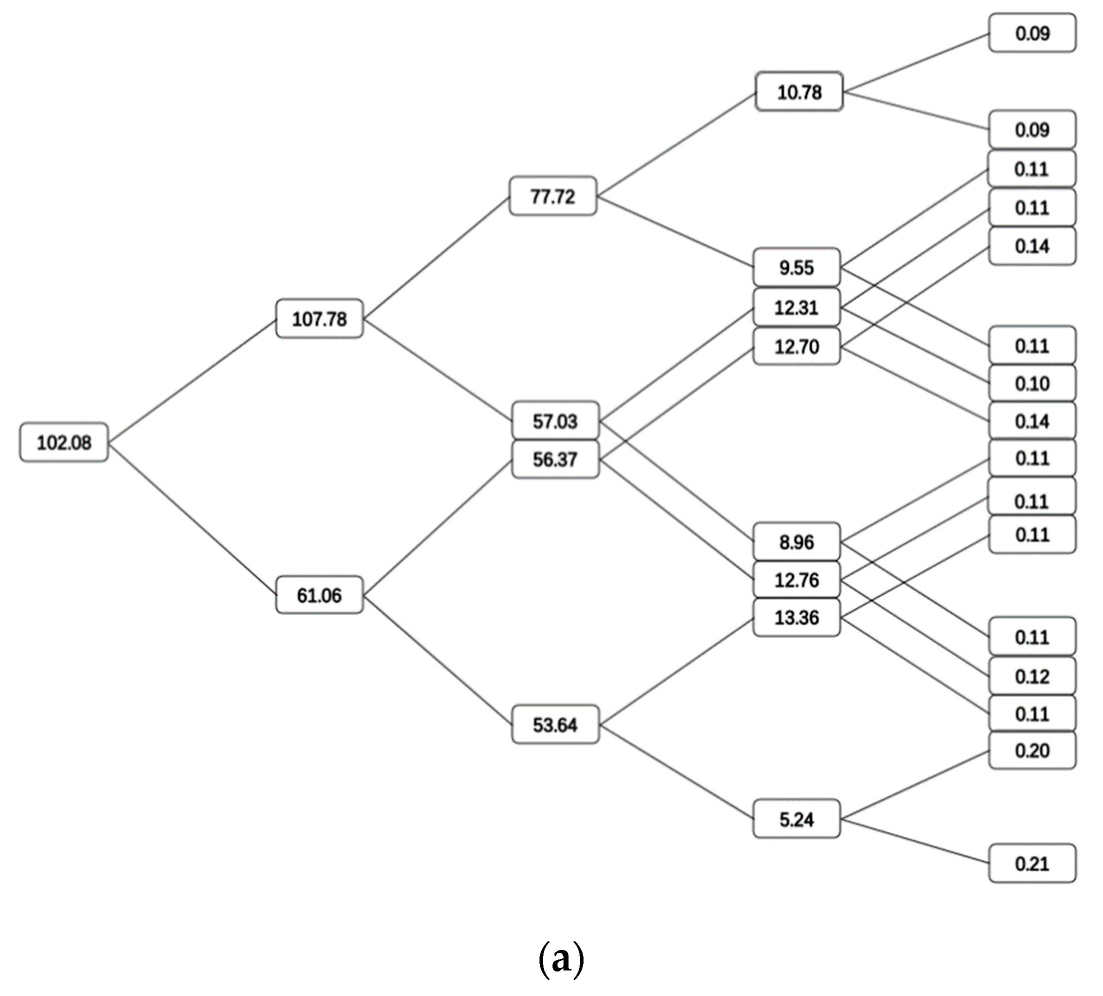
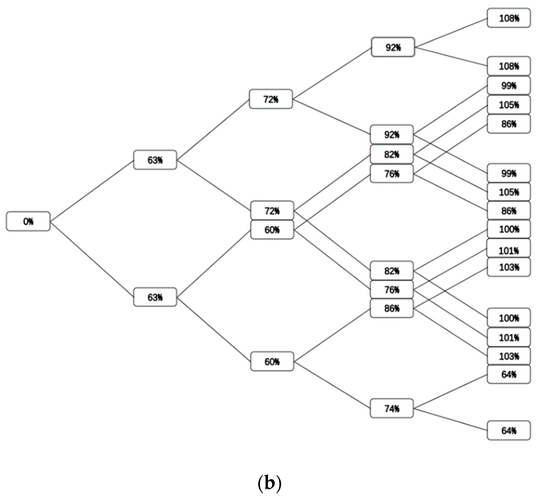
In this paper, we project the future marginal abatement costs (MACs) using EZ climate model and calculate average mitigation rates (AMRs). Moreover, we consider two climate policies: the economically optimal policy and the 1.5 °C temperature increase constraint policy. Our dataset is based on the latest SSP storylines. In Section 4, the SSP3 serves as a representative case; under the economically optimal policy, the expected MACs for 2015, 2030, 2060, 2100, and 2200 are: $102.08, $84.42, $61.19, $10.71, and $0.12, respectively, and the expected AMRs are: 0%, 63%, 66%, 81%, and 96%, respectively. However, Daniel et al. [21] calculated the expected MACs for the same periods at $126.51, $136.40, $130.06, $99.54, $25.02, respectively, with expected AMRs of 0%, 69%, 74.5%, 83%, and 94.4%, respectively. Daniel et al. [21] considered catastrophic climate damage to occur when the temperature increase reaches 6 °C; this would be the equivalent of the 6 °C temperature increase constraint policy. However, our study does not consider temperature constraint under the representative case. That leads to the differences in the studies. Therefore, both MACs and AMRs are higher in the study of Daniel et al. [21], with the exception of AMR in 2200.

The expected MAC and AMR under the five SSPs subject to the “economically optimal” policy and the 1.5 °C temperature increase constraint policy are presented. Both MAC and AMR are related to the emission reduction rate. According to the formulae of MAC and AMR, when the emission reduction rate increases, AMR also increases. The MAC may either increase or decrease. The values of MAC before 2100 and AMR of all periods are greater under the 1.5 °C policy compared to the economically optimal policy. This means that stricter climate policies are generally associated with greater MACs and AMRs. Comparing the expected MACs of the five SSPs, the MAC values of SSP3 (Regional Rivalry) and SSP5 (Fossil-Fueled Development) are highest, while the MAC values of SSP1 (Sustainability) and SSP4 (Inequality) are lowest. SSP2 (Middle of the Road) shows a moderate decreasing trend with respect to the MAC. This means that in a world developing towards regional rivalry (SSP3) or fossil-fueled development (SSP5) with high mitigation pressure, the MAC values approximately double compared with the sustainability (SSP1) and inequality (SSP4) storylines with low mitigation pressure.

The sensitivity analyses for uncertainty parameters are also provided. The time preference rate and intertemporal substitution elasticity have the most significant impact on the MACs. The MAC and time preference rate are significantly inversely correlated. This means that a higher time preference rate is associated with a higher concern for the welfare of the current generation. Therefore, a lower reduction in current emissions is associated with a lower MAC. The reverse is also true. The MAC is positively correlated with intertemporal substitution elasticity. This means that a greater intertemporal substitution elasticity is associated with a greater willingness by the agent to delay consumption. To increase the future consumption, the agent is willing to reduce emissions more now, yielding a higher MAC. Since researchers have not reached consensus on the values of the time preference rate and intertemporal substitution elasticity, the most effective values of the two parameters have not yet been identified. Both exogenous and endogenous technological improvements negatively impact the MAC. This means that emission reduction technology improvements support a decrease in emission reduction costs under identical emission reduction measures.

This study explores the impact of uncertainty in future socioeconomic development on major outcomes related to climate change, extending previous studies. First, we project the future MACs under the five SSPs using the EZ climate model. This contrasts with the study of Daniel et al. [21], which projected future carbon prices given by MACs using the EZ climate model under RCPs. Those RCPs, however, did not make socio-economic assumptions driving future emissions and simply reflect different potential climate outcomes. Second, our study differs from other studies, in that it indicates a general downward trend in carbon prices. In our study, the optimal price per unit of CO₂ emission permit should be equal to the MAC in a perfectly competitive market based on marginal cost theory. Therefore, the trends associated with future carbon prices are consistent with the trend of MACs, showing a trend of gradual decreasing or first increasing and then decreasing. Yang et al. [14] updated the SCCs, which measure the present value of future economic damage caused by each additional ton of carbon emission, under five SSPs using the DICE model. That established a benchmark for carbon pricing. Therefore, the future carbon prices given by the SCCs show a trend of gradual increasing under the five SSPs. In addition, the MACs decline over time, as the “insurance” value of mitigation declines, and technological improvement makes emission reductions less expensive in our model. This is because the MAC mainly depends on the progress of emission reduction technology under identical emission reduction measure and the replacement of those measures. The MACs decrease as the technology changes under an identical emission reduction measure. Under different emission reduction measures, companies often first choose lower abatement cost measures. Even less expensive cost measures are selected after the low-cost emission reduction measures have been exhausted, leading to an increase in MACs. Under the dual influence of these two effects, the expected MAC path shows a decreasing trend, or an initial increase and then decrease. Along the optimal mitigation path, Gollier [30] proposed that frontloading the abatement effort is equivalent to an investment with a cost and a benefit that are equal to the present and future MAC and the marginal investment should have a zero net present value, causing the growth rate of MAC to be equal to the discount rate. The trend associated with the MAC is increasing. In summary, our study considers the advancement and use of different mitigation technologies, and therefore, provides a more comprehensive consideration of the factors influencing MAC.

Two important implications emerge from this study. The MAC value provides a carbon price benchmark for policy makers having different attitudes towards an unknown future. The estimated AMR can be used to formulate carbon mitigation strategies under a specific climate goal.

Like all studies, this one has some methodological limitations. The Epstein-Zin utility is defined by the complete branching tree of possible futures growing out of the present moment. If we divide the long-term future into 40 periods, and make a binary choice for each period, the tree of possible futures has $2^{40}$ branches. To calculate the utility of the first period, it is necessary to follow each of $2^{40}$ branches to its endpoint [21]. In response, our study models very few time periods, thereby losing the long-term modeling of climate and economic dynamics found in IAMs. In addition, this study does not consider relevant behavioral economics concepts such as psychological costs and “sludge”, where “sludge” is typically understood as frictions that make good decisions harder. However, these factors can impede end users in any process, ultimately reducing welfare [31,32,33]. A final recommendation is to consider psychological costs and “sludge” in future climate modeling.