
Process Planning, Scheduling, and Layout Optimization for Multi-Unit Mass-Customized Products in Sustainable Reconfigurable Manufacturing System


Abstract
:1. Introduction
- including the environmental sustainability for this integrated production management problem in RMS, which is limited in previous research;
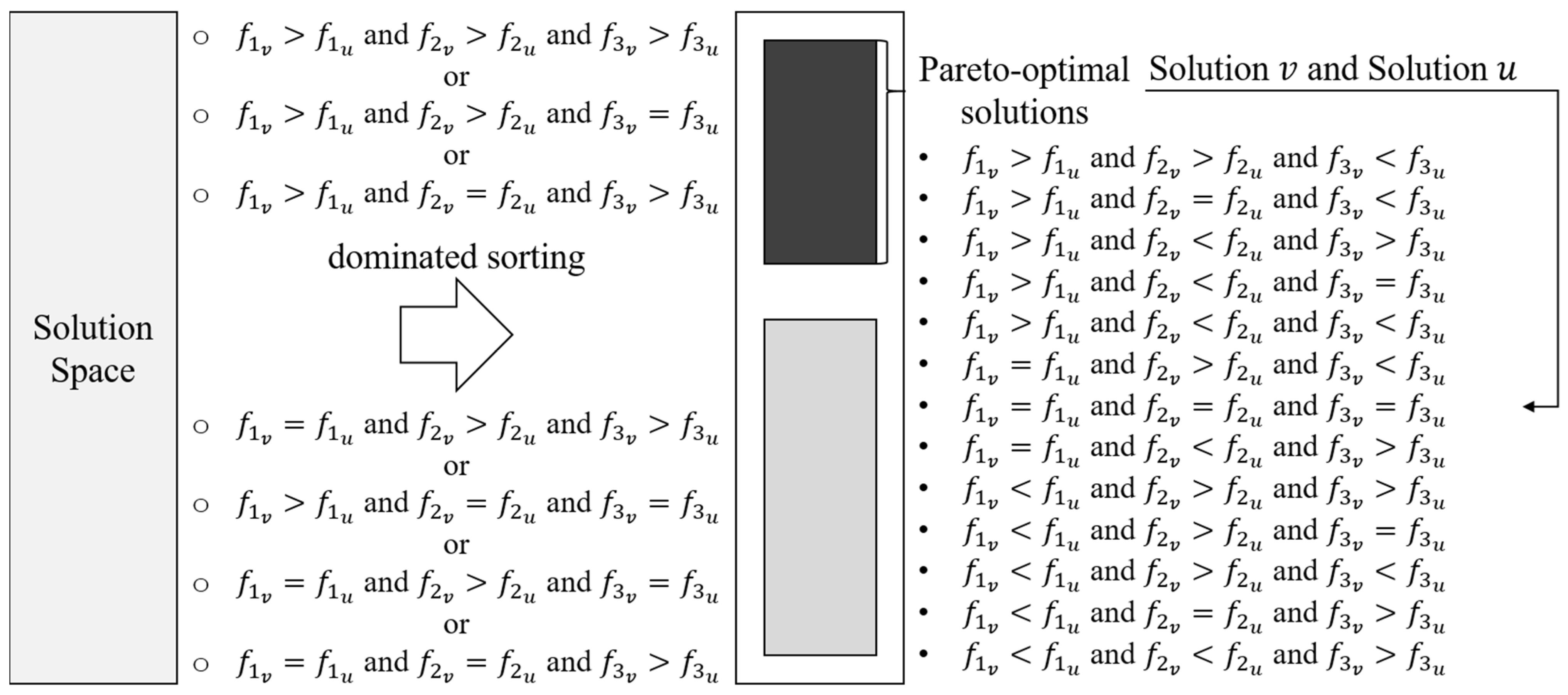
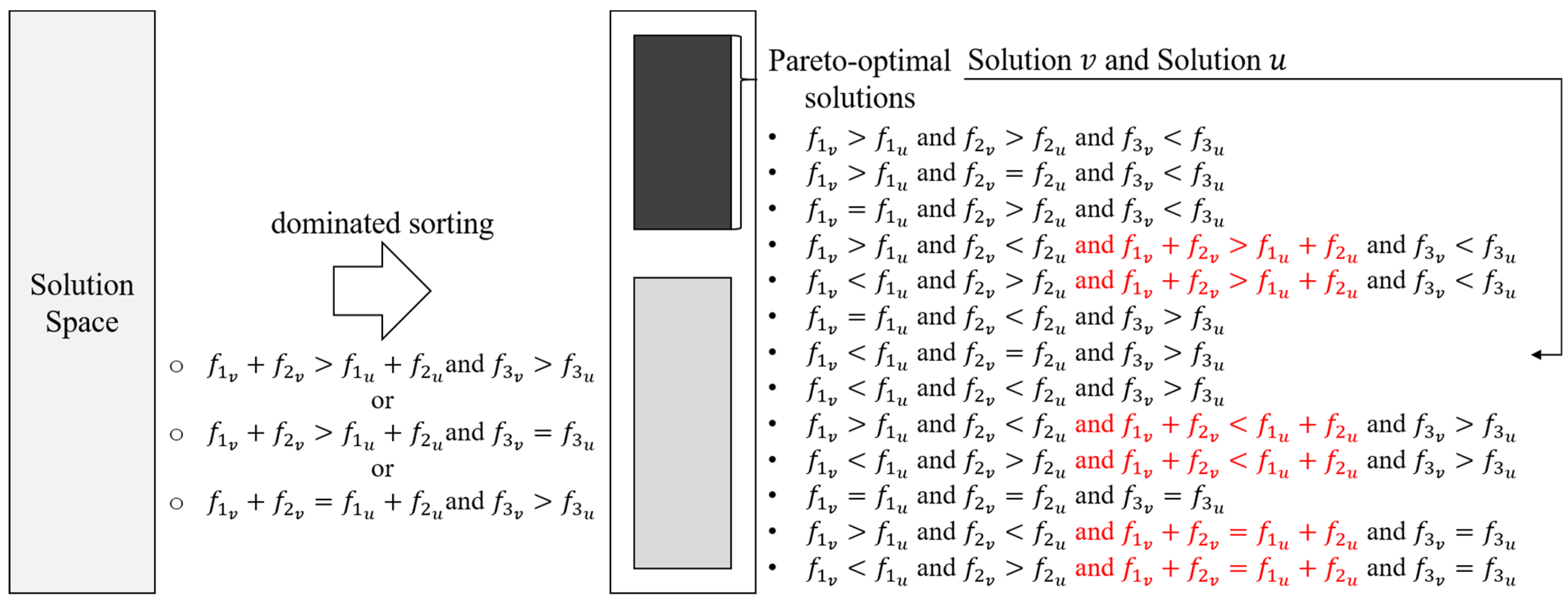
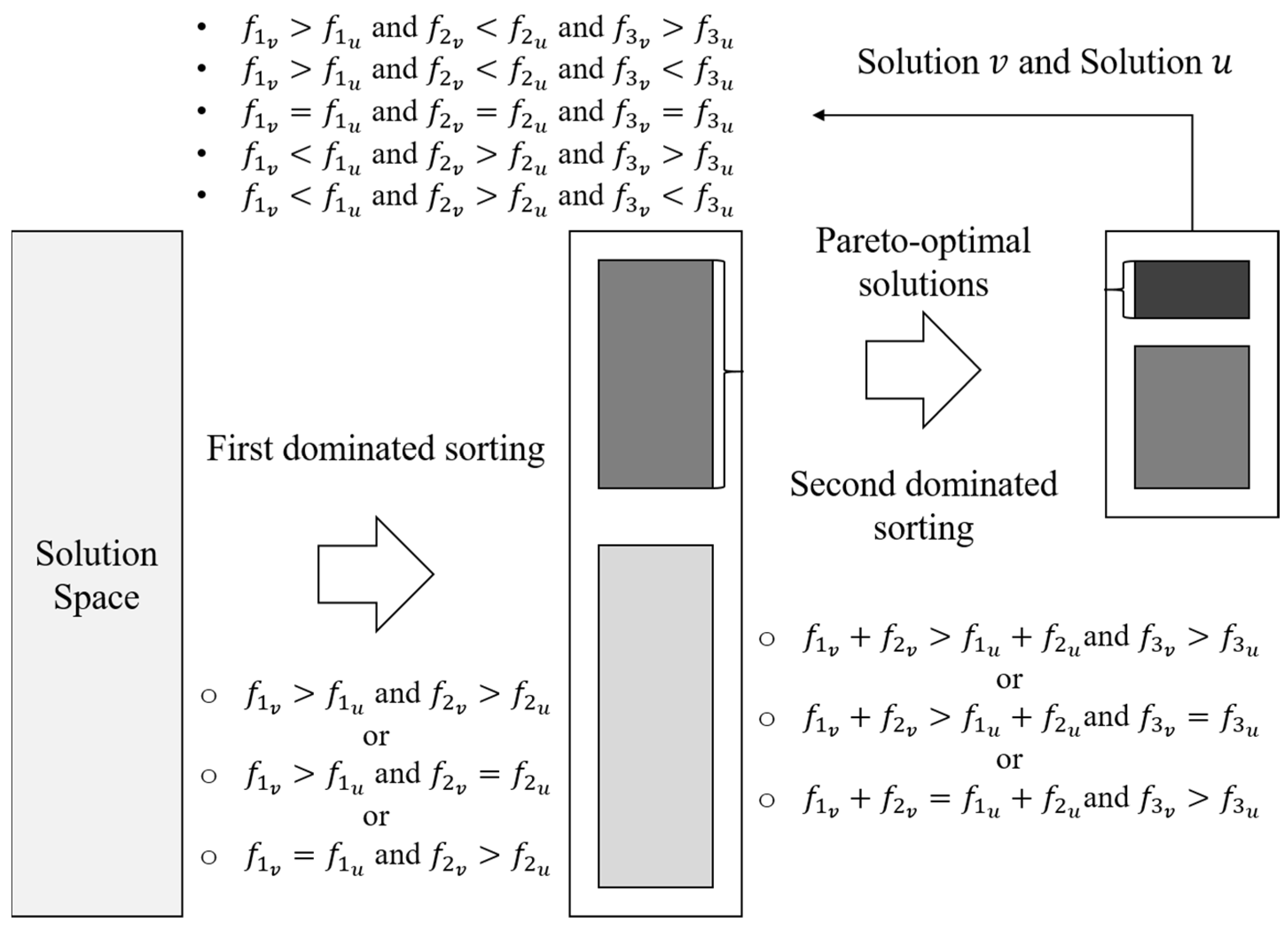
- modifying the Pareto efficiency by combining the characteristics of this problem to get a reasonable number of Pareto-optimal solutions for decision makers; and
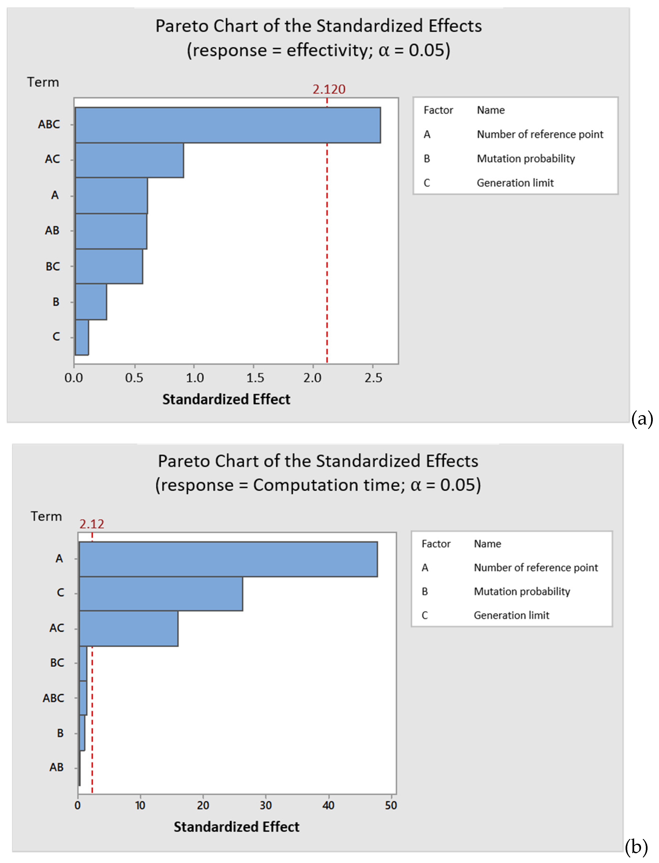
- surveying the appropriate parameters to design a decent heuristic approach in order to solve this problem effectively and efficiently.
2. Literature Review
3. Problem Formulation
3.1. Assumptions
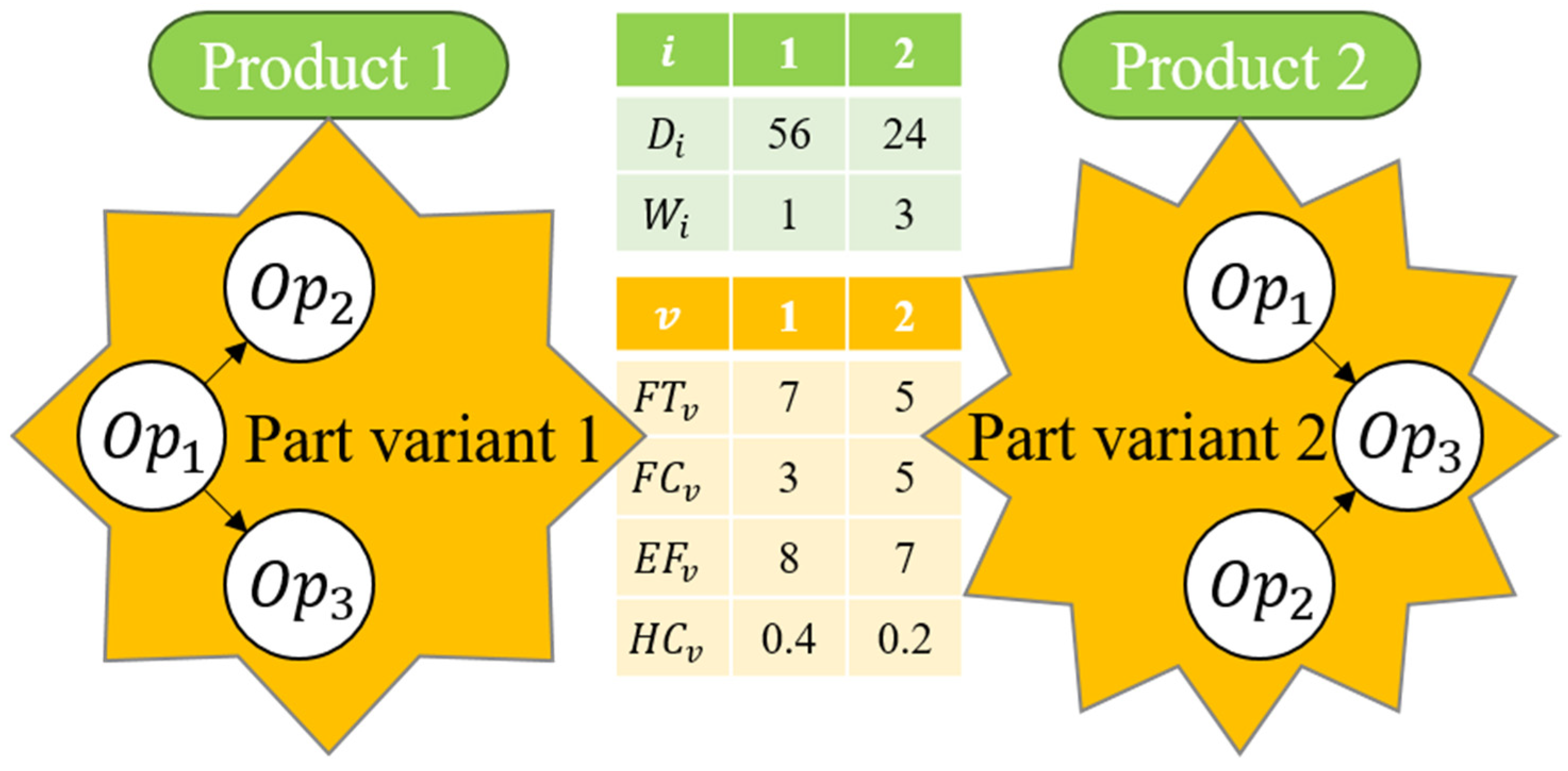
- Parameters about a WIP’s transportation time, cost, energy consumption, and holding cost are only dependent on the type of part variant this WIP belongs to;
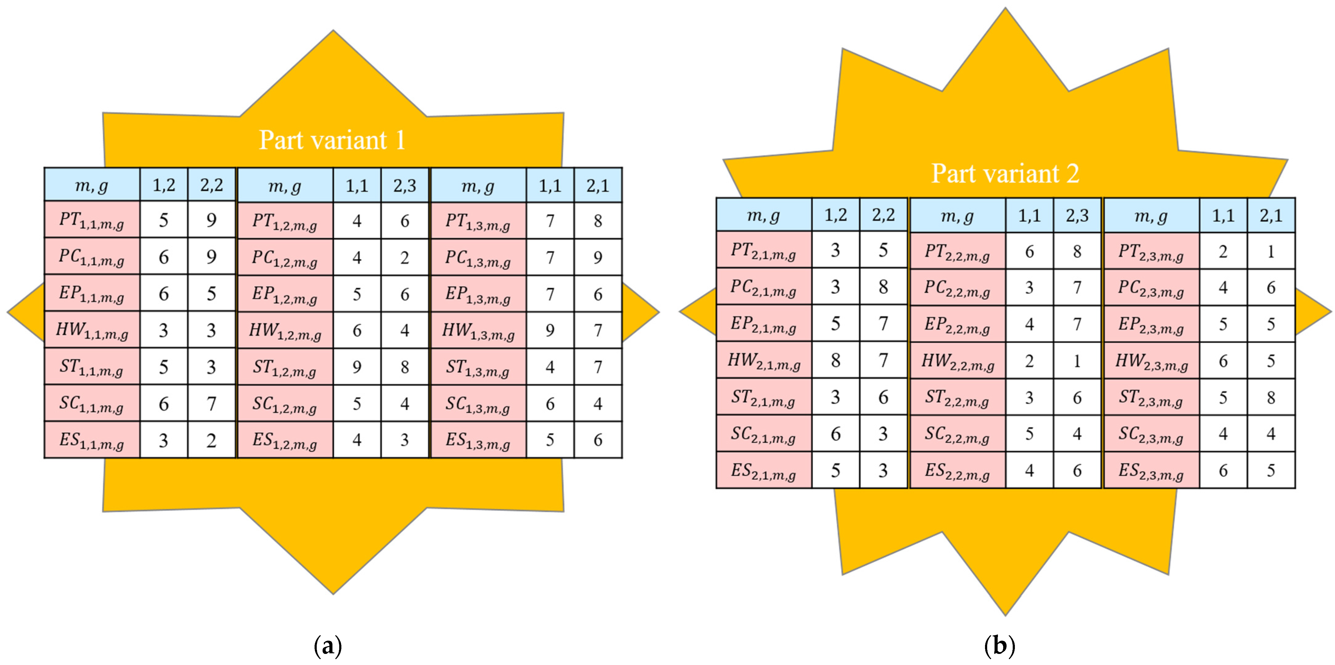
- Parameters about an operation’s processing time, processing cost, processing energy consumption, hazardous waste, setup time, setup cost, and setup energy consumption are dependent on the type of part variant the corresponding WIP belongs to, the kind of this operation, the executing machine, and the configuration;
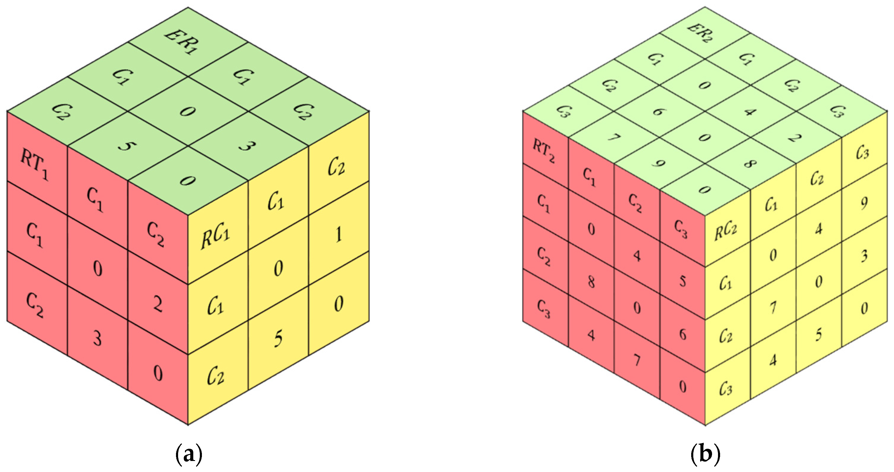
- Parameters about reconfiguration time, cost, and energy consumption on a machine depend on the former configuration and the latter configuration;
- Energy consumed from different activities is quantified with the same unit, which can be added directly to estimate the amount of GHG emissions;
- Parts and the final mass-customized products are qualified without any defect during production in RMS;
- All machines are idle without configurations and setups at the beginning of the task to produce a given number of mass-customized products; and
- All the raw materials and handling devices are available.
3.2. Notations
3.2.1. Sets and Indices
3.2.2. Parameters
3.2.3. Independent Decision Variables
3.2.4. Auxiliary Decision Variables
3.3. Mathematical Model
3.3.1. Objective Functions
- The total penalty of tardiness for all the delayed products accomplished after the due date;
- The total cost including the total setup cost, the total processing cost, the total WIP transport cost, the total WIP holding cost, the total machine reconfiguration cost, and the total layout reconfiguration cost; and
- The value of the environment indicator defined as the aggregate of the normalized hazardous waste item (the ratio of the total amount of hazardous waste and the allowed amount of hazardous waste) and the normalized GHG emissions item (the ratio of the total amount of GHG emissions and the allowed amount of GHG emissions).
3.3.2. Constraints
4. Numerical Experiment
4.1. Modified Pareto Efficiency
4.2. Exact Pareto-Optimal Solutions Obtained from Brute-Force Search
4.3. Comparison with Exact Pareto-Optimal Solutions for No Environmental Indicator Model
5. Approximate Optimization
5.1. Approximate Pareto-Optimal Solutions Obtained from NSGA-III
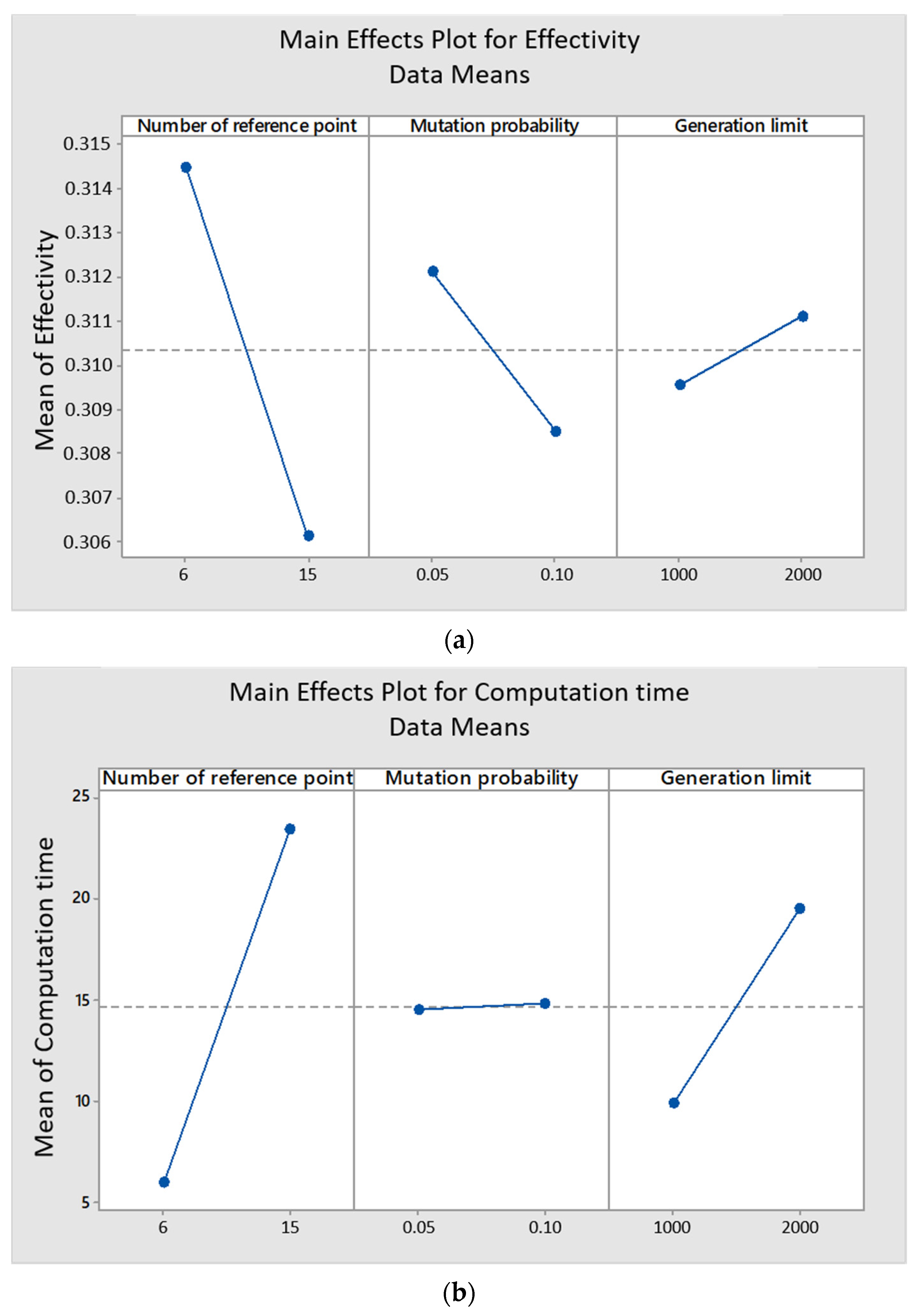
5.2. Parameter Tunning
6. Conclusions
Author Contributions
Funding
Institutional Review Board Statement
Informed Consent Statement
Data Availability Statement
Acknowledgments
Conflicts of Interest
References
- Wang, Q.; Qi, P.; Li, S. A Concurrence Optimization Model for Low-Carbon Product Family Design and the Procurement Plan of Components under Uncertainty. Sustainability 2021, 13, 10764. [Google Scholar] [CrossRef]
- Rehman, A.U.; Mian, S.H.; Umer, U.; Usmani, Y.S. Strategic Outcome Using Fuzzy-AHP-Based Decision Approach for Sustainable Manufacturing. Sustainability 2019, 11, 6040. [Google Scholar] [CrossRef] [Green Version]
- Mehrabi, M.G.; Ulsoy, A.G.; Koren, Y. Reconfigurable manufacturing systems: Key to future manufacturing. J. Intell. Manuf. 2000, 11, 403–419. [Google Scholar] [CrossRef]
- da Silveira, G.J.; Borenstein, D.; Fogliatto, F. Mass customization: Literature review and research directions. Int. J. Prod. Econ. 2001, 72, 1–13. [Google Scholar] [CrossRef]
- Noël, C.; Meaude, M.; Daaboul, J. La customization de masse, est-elle une approche de production durable? In Proceedings of the 17ème colloque national S-mart AIP-PRIMECA, Université Polytechnique Hauts-de-France [UPHF], LAVAL VIRTUAL WORLD, Laval, France, 31 March–2 April 2021; p. hal-03296126. [Google Scholar]
- Bortolini, M.; Galizia, F.G.; Mora, C. Reconfigurable manufacturing systems: Literature review and research trend. J. Manuf. Syst. 2018, 49, 93–106. [Google Scholar] [CrossRef]
- Deb, K.; Jain, H. An Evolutionary Many-Objective Optimization Algorithm Using Reference-Point-Based Nondominated Sorting Approach, Part I: Solving Problems With Box Constraints. IEEE Trans. Evol. Comput. 2013, 18, 577–601. [Google Scholar] [CrossRef]
- Bensmaine, A.; Dahane, M.; Benyoucef, L. A non-dominated sorting genetic algorithm based approach for optimal machines selection in reconfigurable manufacturing environment. Comput. Ind. Eng. 2013, 66, 519–524. [Google Scholar] [CrossRef]
- Hasan, F.; Jain, P.K.; Kumar, D. Optimum configuration selection in Reconfigurable Manufacturing System involving multiple part families. OPSEARCH 2013, 51, 297–311. [Google Scholar] [CrossRef]
- Musharavati, F.; Hamouda, A. Simulated annealing with auxiliary knowledge for process planning optimization in reconfigurable manufacturing. Robot. Comput. Manuf. 2011, 28, 113–131. [Google Scholar] [CrossRef]
- Touzout, F.A.; Benyoucef, L. Multi-objective multi-unit process plan generation in a reconfigurable manufacturing environment: A comparative study of three hybrid metaheuristics. Int. J. Prod. Res. 2019, 57, 7520–7535. [Google Scholar] [CrossRef]
- Roshanaei, V.; Azab, A.; Elmaraghy, H. Mathematical modelling and a meta-heuristic for flexible job shop scheduling. Int. J. Prod. Res. 2013, 51, 6247–6274. [Google Scholar] [CrossRef]
- Valente, A.; De Simone, L.; Carpanzano, E.; Ferraris, F. A methodology for static and dynamic scheduling of automation tasks in reconfigurable production systems. CIRP J. Manuf. Sci. Technol. 2012, 5, 241–253. [Google Scholar] [CrossRef]
- Prasad, D.; Jayswal, S. Scheduling in reconfigurable manufacturing system for uncertainty in decision variables. Mater. Today Proc. 2018, 5, 18451–18458. [Google Scholar] [CrossRef]
- Mahmoodjanloo, M.; Tavakkoli-Moghaddam, R.; Baboli, A.; Bozorgi-Amiri, A. Flexible job shop scheduling problem with reconfigurable machine tools: An improved differential evolution algorithm. Appl. Soft Comput. 2020, 94, 106416. [Google Scholar] [CrossRef]
- Ausaf, M.F.; Gao, L.; Li, X. Optimization of multi-objective integrated process planning and scheduling problem using a priority based optimization algorithm. Front. Mech. Eng. 2015, 10, 392–404. [Google Scholar] [CrossRef]
- Dou, J.; Li, J.; Su, C. Bi-objective optimization of integrating configuration generation and scheduling for reconfigurable flow lines using NSGA-II. Int. J. Adv. Manuf. Technol. 2016, 86, 1945–1962. [Google Scholar] [CrossRef]
- Morganti, L.; Benderbal, H.H.; Benyoucef, L.; Bortolini, M.; Galizia, F.G. A New Process Quality-based Multi-objective Multi-part Approach for the Integrated Process Planning and Scheduling (IPPS) Problem in Reconfigurable Manufacturing Environment. IFAC-PapersOnLine 2020, 53, 10755–10760. [Google Scholar] [CrossRef]
- Maganha, I.; Silva, C. A Theoretical Background for the Reconfigurable Layout Problem. Procedia Manuf. 2017, 11, 2025–2033. [Google Scholar] [CrossRef]
- Haddou-Benderbal, H.; Dahane, M.; Benyoucef, L. Layout evolution effort for product family in Reconfigurable Manufacturing System design. IFAC-PapersOnLine 2017, 50, 10166–10171. [Google Scholar] [CrossRef]
- Benderbal, H.H.; Dahane, M.; Benyoucef, L. Exhaustive Search Based Heuristic for Solving Machine Layout Problem in Reconfigurable Manufacturing System Design. IFAC-PapersOnLine 2018, 51, 78–83. [Google Scholar] [CrossRef]
- Benderbal, H.H.; Benyoucef, L. A New Hybrid Approach for Machine Layout Design Under Family Product Evolution for Reconfigurable Manufacturing Systems. IFAC-PapersOnLine 2019, 52, 1379–1384. [Google Scholar] [CrossRef]
- Gao, S.; Daaboul, J.; Le Duigou, J. Layout and scheduling optimization problem for a reconfigurable manufacturing system. Int. J. Ind. Eng. Manag. 2021, 12, 165–177. [Google Scholar] [CrossRef]
- Sabioni, R.C.; Daaboul, J.; Le Duigou, J. Concurrent optimisation of modular product and Reconfigurable Manufacturing System configuration: A customer-oriented offer for mass customisation. Int. J. Prod. Res. 2021, 1–17. [Google Scholar] [CrossRef]
- Ghanei, S.; AlGeddawy, T. An Integrated Multi-Period Layout Planning and Scheduling Model for Sustainable Reconfigurable Manufacturing Systems. J. Adv. Manuf. Syst. 2020, 19, 31–64. [Google Scholar] [CrossRef]
- Kurniadi, K.A.; Ryu, K. Development of Multi-Disciplinary Green-BOM to Maintain Sustainability in Reconfigurable Manufacturing Systems. Sustainability 2021, 13, 9533. [Google Scholar] [CrossRef]
- Touzout, F.A.; Benyoucef, L.; Benderbal, H.H.; Dahane, M. A hybrid multi-objective based approach for sustainable process plan generation in a reconfigurable manufacturing environment. In Proceedings of the 2018 IEEE 16th International Conference on Industrial Informatics (INDIN), Porto, Portugal, 18–20 July 2018; pp. 343–348. [Google Scholar]
- Touzout, F.A.; Benyoucef, L. Sustainable multi-unit process plan generation in a reconfigurable manufacturing environment: A comparative study of three hybrid-meta-heuristics. In Proceedings of the 2018 IEEE 23rd International Conference on Emerging Technologies and Factory Automation (ETFA), Turin, Italy, 4–7 September 2018; Volume 1, pp. 661–668. [Google Scholar]
- Khezri, A.; Benderbal, H.H.; Benyoucef, L. A Sustainable Reconfigurable Manufacturing System Designing With Focus On Environmental Hazardous Wastes. In Proceedings of the 2019 24th IEEE International Conference on Emerging Technologies and Factory Automation (ETFA), Zaragoza, Spain, 10–13 September 2019; pp. 317–324. [Google Scholar]
- Lamy, D.; Schulz, J.; Zaeh, M.F. Energy-aware scheduling in reconfigurable multiple path shop floors. Procedia CIRP 2020, 93, 1007–1012. [Google Scholar] [CrossRef]
- Hees, A.; Reinhart, G. Approach for Production Planning in Reconfigurable Manufacturing Systems. Procedia CIRP 2015, 33, 70–75. [Google Scholar] [CrossRef]
- Johannes, C.; Wichmann, M.G.; Spengler, T.S. Energy-oriented production planning with time-dependent energy prices. Procedia CIRP 2019, 80, 245–250. [Google Scholar] [CrossRef]
- Koren, Y.; Gu, X.; Guo, W. Reconfigurable manufacturing systems: Principles, design, and future trends. Front. Mech. Eng. 2018, 13, 121–136. [Google Scholar] [CrossRef] [Green Version]
- Waschneck, B.; Reichstaller, A.; Belzner, L.; Altenmüller, T.; Bauernhansl, T.; Knapp, A.; Kyek, A. Optimization of global production scheduling with deep reinforcement learning. Procedia CIRP 2018, 72, 1264–1269. [Google Scholar] [CrossRef]
- Yang, S.; Xu, Z. Intelligent scheduling and reconfiguration via deep reinforcement learning in smart manufacturing. Int. J. Prod. Res. 2021, 1–18. [Google Scholar] [CrossRef]


| Abbreviations | Implication |
|---|---|
| RMS | reconfigurable manufacturing system |
| MC | mass customization |
| NSGA-II | non-dominated sorting genetic algorithm II |
| NSGA-III | non-dominated sorting genetic algorithm III |
| AMOSA | archived multi-objective simulated annealing |
| GHG | greenhouse gases |
| WIP | work in progress |
| FJSP | flexible job-shop scheduling |
| NP-hard | non-deterministic polynomial-time hardness |
| the total setup cost | |
| the total processing cost | |
| the total WIP transport cost | |
| the total WIP holding cost | |
| the total machine reconfiguration cost | |
| the total layout reconfiguration cost | |
| the total amount of hazardous waste | |
| the allowed amount of hazardous waste | |
| the total amount of GHG emissions | |
| the allowed amount of GHG emissions |
| Solutions | First Objective Function | Second Objective Function | Third Objective Function |
|---|---|---|---|
| Solution 1 | 3 | 70 | 0.9811320754716981 |
| Solution 2 | 10 | 69 | 0.8662131519274376 |
| Solution 3 | 10 | 69 | 0.8662131519274376 |
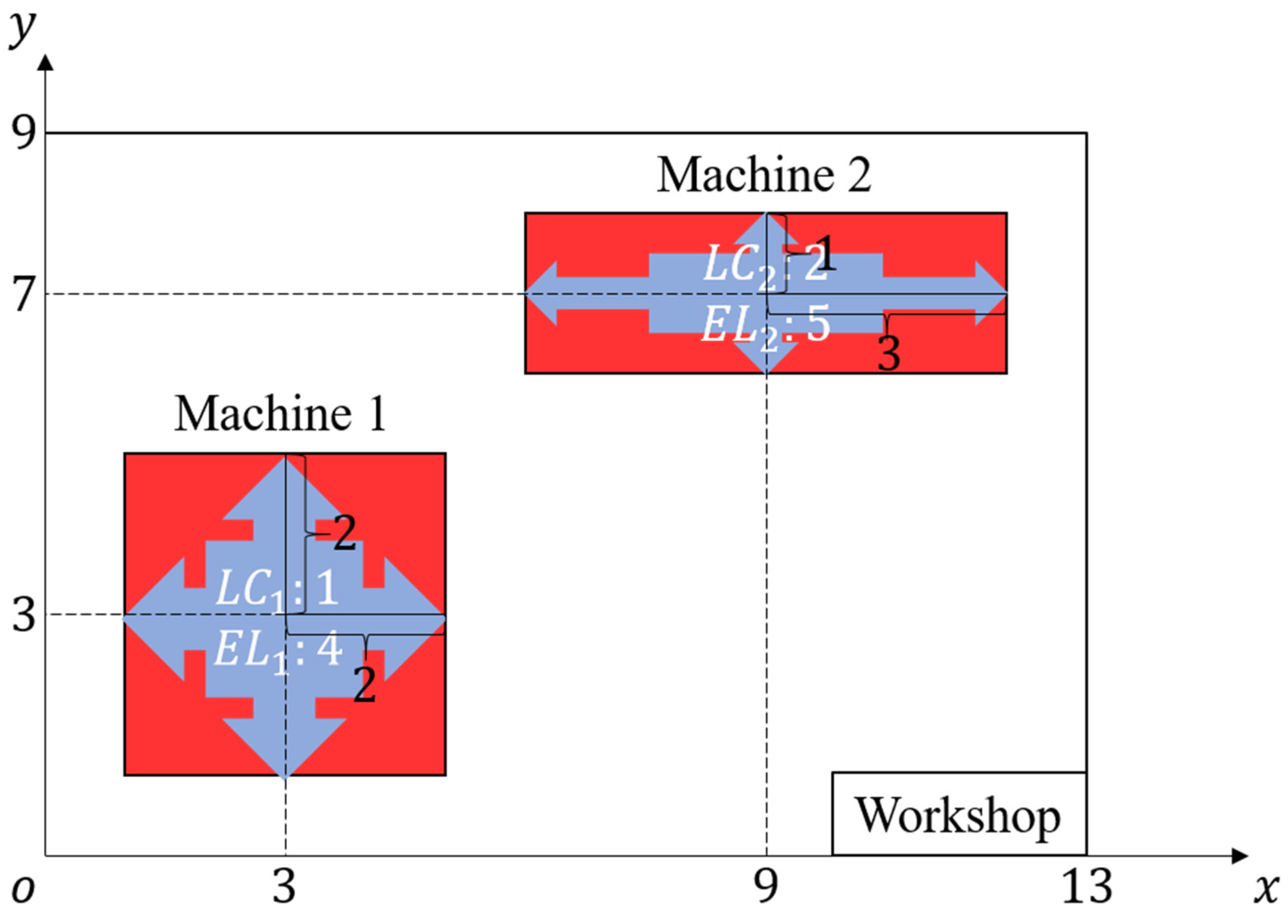
| Solutions | Machines | Position on the X-Coordinate | Position on the Y-Coordinate |
|---|---|---|---|
| Solution 1 | Machine 1 | 3 | 3 |
| Machine 2 | 9 | 7 | |
| Solution 2 | Machine 1 | 3 | 3 |
| Machine 2 | 9 | 7 | |
| Solution 3 | Machine 1 | 3 | 3 |
| Machine 2 | 9 | 7 |
| Solutions | Independent Decision Variables | ||||||
|---|---|---|---|---|---|---|---|
| Solution 1 | 0 | 1 | 2 | 0 | 1 | 2 | |
| 1 | 1 | 1 | 0 | 0 | 0 | ||
| 1 | 2 | 0 | 1 | 0 | 0 | ||
| 3 | 27 | 45 | 3 | 12 | 23 | ||
| Solution 2 | 0 | 1 | 2 | 0 | 1 | 2 | |
| 0 | 0 | 0 | 0 | 0 | 0 | ||
| 1 | 0 | 0 | 1 | 0 | 0 | ||
| 31 | 48 | 56 | 3 | 12 | 23 | ||
| Solution 3 | 0 | 2 | 1 | 0 | 1 | 2 | |
| 0 | 0 | 0 | 0 | 0 | 0 | ||
| 1 | 0 | 0 | 1 | 0 | 0 | ||
| 31 | 43 | 59 | 3 | 12 | 23 | ||
| Solutions | First Objective Function | Second Objective Function |
|---|---|---|
| Solution 1 | 3 | 70 |
| Solution 2 | 10 | 69 |
| Solution 3 | 10 | 69 |
| Solution 4 | 36 | 63 |
| Solution 5 | 36 | 63 |
| Solution 6 | 36 | 63 |
| Solution 7 | 36 | 63 |
| Solutions | Machines | Position on the X-Coordinate | Position on the Y-Coordinate |
|---|---|---|---|
| Solution 1 | Machine 1 | 3 | 3 |
| Machine 2 | 9 | 7 | |
| Solution 2 | Machine 1 | 3 | 3 |
| Machine 2 | 9 | 7 | |
| Solution 3 | Machine 1 | 3 | 3 |
| Machine 2 | 9 | 7 | |
| Solution 4 | Machine 1 | 3 | 3 |
| Machine 2 | 9 | 7 | |
| Solution 5 | Machine 1 | 3 | 3 |
| Machine 2 | 9 | 7 | |
| Solution 6 | Machine 1 | 3 | 3 |
| Machine 2 | 9 | 7 | |
| Solution 7 | Machine 1 | 3 | 3 |
| Machine 2 | 9 | 7 |
| Solutions | Independent Decision Variables | ||||||
|---|---|---|---|---|---|---|---|
| Solution 1 | 0 | 1 | 2 | 0 | 1 | 2 | |
| 1 | 1 | 1 | 0 | 0 | 0 | ||
| 1 | 2 | 0 | 1 | 0 | 0 | ||
| 3 | 27 | 45 | 3 | 12 | 23 | ||
| Solution 2 | 0 | 1 | 2 | 0 | 1 | 2 | |
| 0 | 0 | 0 | 0 | 0 | 0 | ||
| 1 | 0 | 0 | 1 | 0 | 0 | ||
| 31 | 48 | 56 | 3 | 12 | 23 | ||
| Solution 3 | 0 | 2 | 1 | 0 | 1 | 2 | |
| 0 | 0 | 0 | 0 | 0 | 0 | ||
| 1 | 0 | 0 | 1 | 0 | 0 | ||
| 31 | 43 | 59 | 3 | 12 | 23 | ||
| Solution 4 | 0 | 1 | 2 | 0 | 1 | 2 | |
| 0 | 0 | 0 | 0 | 0 | 0 | ||
| 1 | 0 | 0 | 1 | 0 | 0 | ||
| 5 | 44 | 52 | 13 | 22 | 33 | ||
| Solution 5 | 0 | 1 | 2 | 0 | 1 | 2 | |
| 0 | 0 | 0 | 0 | 0 | 0 | ||
| 1 | 0 | 0 | 1 | 0 | 0 | ||
| 11 | 44 | 52 | 3 | 22 | 33 | ||
| Solution 6 | 0 | 2 | 1 | 0 | 1 | 2 | |
| 0 | 0 | 0 | 0 | 0 | 0 | ||
| 1 | 0 | 0 | 1 | 0 | 0 | ||
| 5 | 39 | 55 | 13 | 22 | 33 | ||
| Solution 7 | 0 | 2 | 1 | 0 | 1 | 2 | |
| 0 | 0 | 0 | 0 | 0 | 0 | ||
| 1 | 0 | 0 | 1 | 0 | 0 | ||
| 11 | 39 | 55 | 3 | 22 | 33 | ||
| Solutions | First Objective Function | Second Objective Function | Third Objective Function |
|---|---|---|---|
| Solution 1 | 6 | 74 | 1.0242587601078168 |
| Solution 2 | 36 | 65 | 0.910411622276029 |
| Solution 3 | 36 | 65 | 0.910411622276029 |
| Solutions | Machines | Position on the X-Coordinate | Position on the Y-Coordinate |
|---|---|---|---|
| Solution 1 | Machine 1 | 3 | 3 |
| Machine 2 | 8 | 7 | |
| Solution 2 | Machine 1 | 3 | 3 |
| Machine 2 | 8 | 7 | |
| Solution 3 | Machine 1 | 3 | 3 |
| Machine 2 | 8 | 7 |
| Solutions | Independent Decision Variables | ||||||
|---|---|---|---|---|---|---|---|
| Solution 1 | 0 | 1 | 2 | 1 | 0 | 2 | |
| 1 | 1 | 1 | 0 | 0 | 0 | ||
| 1 | 2 | 0 | 0 | 1 | 0 | ||
| 3 | 27 | 45 | 3 | 13 | 24 | ||
| Solution 2 | 0 | 1 | 2 | 0 | 1 | 2 | |
| 0 | 0 | 0 | 0 | 0 | 0 | ||
| 1 | 0 | 0 | 1 | 0 | 0 | ||
| 5 | 44 | 52 | 13 | 22 | 33 | ||
| Solution 3 | 0 | 2 | 1 | 0 | 1 | 2 | |
| 0 | 0 | 0 | 0 | 0 | 0 | ||
| 1 | 0 | 0 | 1 | 0 | 0 | ||
| 5 | 39 | 55 | 13 | 22 | 33 | ||
| Solutions | Low Level | High Level |
|---|---|---|
| Number of reference point | 6 | 15 |
| Mutation probability | 0.05 | 0.1 |
| Generation limit | 1000 | 2000 |
Publisher’s Note: MDPI stays neutral with regard to jurisdictional claims in published maps and institutional affiliations. |
© 2021 by the authors. Licensee MDPI, Basel, Switzerland. This article is an open access article distributed under the terms and conditions of the Creative Commons Attribution (CC BY) license (https://creativecommons.org/licenses/by/4.0/).
Share and Cite
Gao, S.; Daaboul, J.; Le Duigou, J. Process Planning, Scheduling, and Layout Optimization for Multi-Unit Mass-Customized Products in Sustainable Reconfigurable Manufacturing System. Sustainability 2021, 13, 13323. https://doi.org/10.3390/su132313323
Gao S, Daaboul J, Le Duigou J. Process Planning, Scheduling, and Layout Optimization for Multi-Unit Mass-Customized Products in Sustainable Reconfigurable Manufacturing System. Sustainability. 2021; 13(23):13323. https://doi.org/10.3390/su132313323
Chicago/Turabian StyleGao, Sini, Joanna Daaboul, and Julien Le Duigou. 2021. "Process Planning, Scheduling, and Layout Optimization for Multi-Unit Mass-Customized Products in Sustainable Reconfigurable Manufacturing System" Sustainability 13, no. 23: 13323. https://doi.org/10.3390/su132313323