Characteristics and Long-Term Trends of Heat Stress for South Africa

Abstract

Increasing air temperature coupled with high humidity due to ongoing climate change across most parts of South Africa is likely to induce and intensify heat exposure, particularly in densely populated areas. The adverse health implications, including heatstroke, are expected to be common and more severe during extreme heat and heat wave events. The present study was carried out to examine heat stress conditions and long-term trends in South Africa. The study aimed to identify geographical locations exposed to elevated heat stress based on over two decades of hourly ground-based data. Selected heat stress indicators were calculated based on Steadman’s apparent temperature (AT in °C). The trends in AT were assessed based on the non-parametric Mann–Kendall (MK) trend test at 5% significance level. Positive trends were detected in 88% of the selected weather stations except in Welkom-FS, Ficksburg-FS, Langebaanweg-WC, Lambertsbaai Nortier-WC, Skukuza-MP, and Thabazimbi-LP. Approximately 47% of the detected positive trends are statistically significant at 5% significant level. Overall, high climatological annual median (ATmed) values (>32 °C) were observed at 42 stations, most of which are in low altitude regions, predominately along the coastlines. The hottest towns with ATmed values in the danger category (i.e., 39–50 °C) were found to be Patensie-EC (41 °C), Pietermaritzburg-KZN (39 °C), Pongola-KZN (39 °C), Knysna-WC (39 °C), Hoedspruit-LP (39 °C), Skukuza-MP (45 °C), and Komatidraai-MP (44 °C). The results provide insight into heat stress characteristics and pinpoint geographical locations vulnerable to heat stress conditions at the community level in South Africa. Such information can be useful in monitoring hotspots of heat stress and contribute to the development of local heat–health adaptation plans.

1. Introduction

Extreme heat is one of the growing weather-related hazards affecting human health and well-being [1]. Most of its effects, which have, over the years, gained significant momentum, are attributed to elevated temperatures resulting from climate change and variability [2,3]. Notably, higher than normal temperatures, coupled with high relative humidity, often cause a sensation of discomfort and sometimes heat stress [4,5]. Heat stress in the present context is defined as the combination of air temperature, radiation, air movements, moisture content, amount of clothing worn, as well as behaviors that induce a physiological inability of the body to maintain its temperature within the heat tolerance limit of 35–37 °C [6]. Regardless of age, gender, or health status, all persons are at risk of heat-related illnesses, including heat stress [7]. However, the vulnerability increases typically in older people, those who are chronically ill, low-income earners, pregnant women, socially isolated individuals, slum and informal settlement dwellers, people working in exposed environments, as well as children under the age of five years [8,9,10]. In addition, athletes and tourists who often cannot fathom the danger of hot weather conditions are also at risk of heat-related illnesses [11,12]. Similarly, people living in urban areas are confronted with a substantial rise in heat stress as compared to those living in the rural–urban fringe or rural areas, since the air temperature in such areas is often higher than in the surrounding due to the urban heat island (UHI) phenomena [13,14]. Demographic growth and ever-increasing urbanization trends suggest the likelihood of many people being placed at increased risk in the future [15,16,17,18].

Prolonged exposure to extreme heat, predominantly during acute heatwaves, can cause a varying degree of medical severities, including oedema, rash, cramps, exhaustion, and heat stroke, which can cause shock, brain damage, as well as internal organ failure, consequently leading to coma [19,20]. Some underlying and pre-existing medical conditions, e.g., asthma, chronic obstructive pulmonary disease, cardiovascular disease, hypertensive diseases, chronic renal failure, diabetes mellitus, mental disorder, and dementia, are exacerbated by extreme heat exposure [1,21,22,23]. Various studies have alluded that exposure to extreme heat and heatwaves conditions are likely to increase mortality and morbidity [24,25,26]. These effects are demonstrated by the deaths of tens of thousands of people in Europe [27,28], China [29,30], the United States of America [31], and other parts of the world [32].

Global model projections indicate that extreme heat and heatwave events are likely to increase in frequency, duration, and intensity well into the future, owing to climate change and variability [33]. As established across various studies, these weather phenomena will be accompanied by heat-related morbidity and mortality [34,35,36,37], to the peril of society. Based on these findings, it is apparent that heat stress is a universal problem even in Africa, where information relating to heat-related illnesses and attributed deaths are not as readily available [32]. This is a cause for concern for the continent, particularly in South Africa, where the observed local climatic factors show an increase in the average temperature of approximately 1.5 times the observed global average of 0.65 °C [38]. Future model projections are also showing a plausible increase in this region [39]. Trends over the past 40 years show a rise of 0.02 °C yr⁻¹ with considerable regional variation [40]. The rate of warming is pronounced in the western region and towards the northeastern parts of South Africa [41]. When further assessing historical data, it is noted that warmer temperatures have dominated in the winter season during 1995–2010, relative to the 1979–1994 period [42]. Moreover, there has been a significant increase in the number of days and nights with relatively high temperatures [41]. Model projections under the A2 scenario indicate that the intense heat and the number of hot days and nights are expected to increase in the near future with adverse implications on human health [43]. Some of the growing evidence of the increase in heat stress exposure in this region was revealed in two local studies; one based on the analysis of heat stress in East London using weather station observation data in the Eastern Cape Province [44] and the second study based on an outdoor and indoor experimental study in the Greater Giyani local municipality in rural Limpopo [45]. For a more comprehensive perspective, Garland et al. [43] provided a model-based regional overview of heat stress conditions over Africa using apparent temperature (AT) and projected an increase in the number of hot days in the region.

As reported in the literature, South Africa is projected to experience hotter temperatures and more frequent and intense heat stress identified by the National Climate Change and Health Adaptation Plan: 2014–2019 as one of the nine environmental risks impacted by climate change [46]. To improve public health response and protect the South African population from extreme heat exposure, the government’s National Climate Change Response Policy (NCCRP) called for the development and implementation of heat-health action plans that must factor population vulnerability and adapt to local conditions [47]. These efforts are in line with the recommendations made by the World Health Organization (WHO) for countries to develop their heat action plans aimed at (1) minimizing increased mortality and morbidity associated with extreme heat and heatwave events, (2) promote careful preparation measures across relevant sectors, including public and medical professional awareness, and (3) mobilize resources to mitigate the health impacts of heat [48]. Berry et al. [49] alluded that identifying and mapping heat stress is one of the key elements in developing and implementing effective and informed heat health plans. Hence, this study investigates climatological patterns and long-term trends of heat stress conditions in South Africa based on meteorological data from 51 weather stations across South Africa using the Steadman’s apparent temperature (hereafter AT) heat index. Steadman’s apparent temperature is a temperature-like combined measure of all the climatic variables that affect human comfort and performance [50]. Specific objectives are to examine heat stress characteristics, identify geographical locations exposed to heat stress conditions, and evaluate long-term trends based on over two decades of hourly ground-based data.

2. Materials and Methods

2.1. Study Area

Geographically, South Africa extends from −22° S to −35° S latitude and from 29° E to 20° E longitude, occupying the southern tip of the African continent [51]. It has approximately 2798 km of coastline that stretches along the South Atlantic and Indian oceans. South Africa covers 1,214,470 km² of land and 4620 km² of water. The country consists of nine provinces, namely the Eastern Cape (EC), Free State (FS), Gauteng (GP), KwaZulu Natal (KZN), Limpopo (LP), Mpumalanga (MP), Northern Cape (NC), North West (NW) and Western Cape (WC)—see Figure 1. The NC is the largest province, covering 30.5% of the total land area. The NC and two neighboring Cape provinces (EC and WC) account for 55% of the country’s land area [52]. The GP is highly urbanized, with a land area of 1.5%. It is also densely populated, with approximately 11 million people [53]. South Africa’s climatic conditions range from arid in the west to humid subtropical in the north and the eastern region, while much of the central part is classified as semi-arid. High temperatures are experienced in the Kalahari Desert regions, lying mainly in the southern parts of the NC and along the border of NW province. Low temperatures are found in high altitude regions of the country [54].

2.2. Datasets

This study examines characteristics of heat stress conditions based on hourly meteorological data collected from 51 selected automatic weather stations (AWS) (See Figure 1), monitored and maintained by the South African weather service (SAWS). These stations were selected based on the availability of continuous data (at least 80%) as well as adequate coverage, e.g., aiming at 5–6 stations per province. The data undergo a series of quality control and assurance tests that identify correct outliers and duplicated values caused by human errors and instrument faults [55]. Three meteorological variables were selected for the analysis, namely the temperature (°C), humidity (%), and wind speed (ms⁻¹). The analyzed data were obtained over a period of 23 years, thus spanning from 1997 to 2020. These data were used to calculate the AT heat index.

2.3. Apparent Temperature Index

Several indices can be used to evaluate heat stress. These can be classified into (1) simple empirical indices, (2) rational indices, and (3) direct indices based on the measurements of environmental parameters [56]. A summary of some of the existing heat indices can be found in Epstein and Moran [57]. This study adopted the modified version of Steadman’s apparent temperature by Buzan et al. [58]. This version was used because it combines temperature, humidity, and wind speed, which provides a more realistic “feel like temperature” for outdoor conditions than what other simplified heat indices could provide, e.g., humidex, which only considers temperature and humidity [59]. The $AT$ index was calculated using Equation (1) [58].

$$AT=T_C+\frac{3.3e_{RH}}{1000}-0.7{\mu }_{10m}-4,$$

(1)

where $T_c$ is the air temperature (°C) or dry bulb temperature (°C), and ${\mu }_{10m}$ is the wind velocity (m/s) measured at 10 m height.$RH(\%)$ is the relative humidity. Vapor and saturated vapor pressure ($e_{RH}$ and $e_{sPa},$ respectively) are in Pascals, as given in Equation (2).

$$e_{RH} ={(RH/100)}_{e_{sPa}}$$

(2)

The current study adopted exposure categories classified by the United States National Weather Service (US NWS) and the National Oceanic and Atmospheric Administration (NOAA) to examine heat stress characteristics based on the combined effect of temperature, humidity, and wind on the South African population as well as to facilitate data interpretation on potential health effects. The categories are accompanied by inherent potential health impacts (NOAA), resulting in each level [60]. The adopted AT categories used in this study are shown in

Table 1. Heat stress categories and potential health effects based on apparent temperature.

US NWS Classification (°C)	Apparent Temperature Range (°C)	US NWS Classified Health Effects
Caution	27–31	Fatigue is possible with prolonged exposure and physical activity
Extreme caution	32–38	Heatstroke, heat cramps, or heat exhaustion is possible
Danger	39–50	Heat cramps or heat exhaustion likely, and heat stroke possible with prolonged exposure and physical activity
Extreme danger	>51	Heatstroke highly likely

and can be classified as follows: caution (27–31 °C), extreme caution (32–38 °C), danger (39–50 °C), and extreme danger (>51 °C). It is worth noting that, while the heat exposure categories were developed for the United States of America’s population, they were adopted for this study, since no similar bands are available for Africa [39]. The same table was used in the AT prediction study by Garland et al. [43].

2.4. Descriptive Statistics

The calculated hourly AT values were averaged to annual AT values. From these, annual median and maximum values of AT were calculated using Equations (3)–(5) [60].

$$f\left(x\right)=a{\left(x-h\right)}^2+k$$

(3)

The maximum value is $k,$ and it occurs at $x=h$

If $n$ is odd, the median is the value at the positive p, where:

$$p=\frac{n+1}{2}$$

(4)

If $n$ is even, the median is the average of the values at positions $p+p+1$, where:

$$p=\frac{n}{2}$$

(5)

The probability of occurrence was calculated based on Equation (6) [61].

$$P_{a=\frac{n_a}{n_2}},$$

(6)

where $P_a$ represents the probability of an event, $n$ is the number of favourable outcomes, and $n_s$ corresponds to the total number of events in the sample space. Furthermore, the coefficient of variation (CoV) [61], which measures the diversification of characteristic distribution, was calculated using Equation (7):

$$V=\frac{S}{X} \times 100\%$$

(7)

To assess the distributional shape of the dataset of each station, skewness and kurtosis descriptive statistics were applied [62,63]. Skewness measures the asymmetry or the distortion symmetric distribution of the data curve. Karl Pearson’s coefficient formula, given by Equation (8), was applied [64].

$$S_K=\frac{\mu -M}{\sigma },$$

(8)

where $\mu$ is the mean,$\sigma$ is the standard deviation, and $M$ is the mode.

A normal distribution results when the median, mean, and mode are equal, where the curve distribution is symmetrical on both sides, and the skewness statistic is close to zero. However, when the mean is greater than the mode, the coefficient of skewness would be positive; otherwise, it is negative [63]. A positively skewed distribution of the data curve is when the skewness value exceeds zero, and an asymmetric tail extends towards higher positive values. On the contrary, a left-skewed distribution has a symmetric tail expanding towards increasingly negative values less than zero [62,63]. Different conditions of skewness can be considered [65], and the following criteria (

Table 2. Conditions for skewness.

Skewness	Distribution
If skewness is less than −1 or greater than 1	A highly skewed distribution
If skewness is between −1 and −0.5 or between 0.5 and 1	A moderately skewed distribution
If skewness is between −0.5 and 0.5	Approximately symmetric (normal) distribution

) were used in this study:

Kurtosis statistics provide the peakedness or flatness of the distribution of the variables, where positive kurtosis implies that the distribution is relatively peaked, while a negative kurtosis indicates a flat distribution [62]. Equation (9) was used to calculate Kurtosis statistics [66].

$${\beta }_{2=\frac{E{(X-\mu )}^4}{(E{(X-\mu {)}^2)}^2}=\frac{{\mu }_4}{{\sigma }^4}},$$

(9)

where $E$ is the expectation operator, $\mu$ is the mean, ${\mu }_4$ is the fourth moment about the mean, and $\sigma$ is the standard deviation.

Three types of distributions of kurtosis statistics are described in

Table 3. Conditions of Kurtosis distribution.

Kurtosis	Curve Type
$\mathrm{If} {\beta }_2=3 or {\gamma }_2=0,$	Curve is mesokurtic
$\mathrm{If} {\beta }_2<3 or {\gamma }_2<0,$	Curve is platykurtic
$\mathrm{If} {\beta }_2>3 or {\gamma }_2>0,$	Curve is leptokurtic

below:

2.5. Trend Analysis Using Mann-Kendall, Theil–Sen ‘s Slope and Z-score

The long-term AT time series over two decades were analyzed using the non-parametric Mann–Kendall (MK) test at 5% significance levels [67,68], and the magnitude of the trends were quantified using the Theil–Sen trend estimator [69,70]. The MK trends were calculated using Equation (10).

$$S={{\displaystyle \sum }}_{k=1}^{n-1}{{\displaystyle \sum }}_{j=i+1}^{n}sgn(x_j-x_i) ,$$

(10)

where $n$ is the number of observations, $x_i$ is the rank for $i$th observations ($i=1, 2\dots n-1)$, $x_j$ is the rank for $j$th observations ($j=i+1, 2\dots n$), and sign function is computed as follows:

$$sgn\left(x_j-x_i\right)=\{\begin{array}{c}+1; if\left(x_j-x_i \right)>0\\ 0; if \left(x_j-x_i \right)=0\\ -1; if \left(x_j-x_i \right)<0\end{array}$$

(11)

The test statistic $S$ is assumed for the series where sample $n>10$ are asymptotically normally distributed with mean $E\left(S\right)$ and variance Var $\left(S\right)$, as follows:

$E\left(S\right)=0$, and

$$\mathrm{Var} \left(S\right)=\frac{n\left(n-1\right)\left(2n+5\right)}{18}$$

(12)

If there is a possibility of a tie in the value of $x$, the variance is computed as follows:

$$\mathrm{Var} \left(S\right)=\frac{n\left(n-1\right)\left(2n+5\right)-{{\displaystyle \sum }}_{i=1}^P{t}_i\left(t_i-1\right)\left(2t_i+5\right)}{18},$$

(13)

where $P$ is the number of tied groups, () indicates the summation over tied groups, and $t_i$ is the number of data values in the $i$th tied group $\left(i=1, 2, 3\dots n\right)$. After the calculation of the Var $\left(S\right)$ of time series data, the standardized $Z_{MK}$ value is calculated using the equation:

$$Z_{MK}\{\begin{array}{c}\frac{S-1}{\sqrt{Var\left(S\right)}};if S>0\\ 0; if S=0\\ \frac{S+1}{\sqrt{Var\left(S\right)}};if S<0\end{array}$$

(14)

The standardized MK test statistic $(Z_{MK})$ follows the standard normal distribution $\left(Z\right)$ with mean zero $\left(\mu =0\right)$ and variance one $({\sigma }^2=1)$. The null hypothesis (no trend) and alternate hypothesis (trend) are tested at 5% significance level. A positive value of $Z_{MK}$ indicates an increasing trend, and a negative value of $Z_{MK}$ indicates a decreasing trend in the time series data [71].

Theil–Sen ‘s Slope (TSS) test is a non-parametric test that is used to estimate the true slope (magnitude) of the trend [69,70,71]. The TSS test estimates the median of all pair-wise slopes among each pair of the points in the time series data (N), which is given as follows:

$$TS{S}_{ij}=\frac{x_j-x_i}{j-i}, j<i,$$

(15)

where $x_j$ and $x_i$ are data values at times $j$ and $i(j>i)$, respectively, for $i=1, 2, 3\dots N.$ Thiel–Sen ‘s slope is the median slope if the $N$ values of slopes and computes as follows:

$$TS{S}_{median}=TS{S}_{\frac{N+1}{2}},\mathrm{if} N\mathrm{is} \mathrm{odd}$$

(16)

$$TS{S}_{median}=\frac{1}{2}\left[TS{S}_{\left(\frac{N}{2}\right)}+TS{S}_{\left(\frac{N+2}{2}\right)}\right],\mathrm{if} N\mathrm{is} \mathrm{even}$$

(17)

The positive (negative) value of $TSS$ indicates a rising (falling) trend, and the zero value of $TSS$ indicates no trend [71].

To determine the existence and significance of the trends, the Z-score was calculated based on Equation (18).

$$Z_i=\frac{x_i-\overline{x}}{\sigma },$$

(18)

where $x_i$ is the value of an observation, $\overline{x}$ is the mean of the distribution of an observation, ${\sigma }_x$ is the standard deviation of the variable, and $Z_i$ is the Z-score of the corresponding outlier. Where a positive/negative value of $Z_i$ indicates an upward/downward trend, and a zero value of $Z_i$ indicates no trend.

2.6. Data Analysis and Visualization

The data analysis was performed with R statistical software, and ArcGIS geographic information mapping tool was used to visualize heat stress conditions. The mapping of geographical locations is essential for decision-makers and relevant stakeholders to visually identify heat stress hotspots that need to be prioritized for adaptation and mitigation strategies [72]. The interpolation was performed using the inverse distance weighting (IDW) technique. Due to ease of implementation and interpretation, IDW is the most widely used interpolation method among various interpolation methodologies (i.e., kriging interpolation, triangulation with linear interpolation, and cubic spline interpolation [73,74]. Its general concept is based on the assumption that the attribute value of an unsampled point is the weighted average of known values within the neighbourhood, and that the weights are inversely related to the distances between the prediction location and the sampled locations [75]. The IDW is represented by Equation (19) [72,73]:

$$Z\left(u\right)={{\displaystyle \sum }}_{i=1}^n{\lambda }_{i}Z\left(u_i\right),$$

(19)

where $u$ is the estimated location, $u$, $i=1, \dots ., n,$ are the locations of the sample points within the search neighborhood, $Z\left(u\right)$ is the inverse distance estimate at the estimation location, $n$ is the number of sample points, ${\lambda }_i, i=1,\dots ,n,$ are the weights assigned to each sample point, and $Z\left(n_i\right),i=1, \dots ,n,$ are the conditioning data at sample points. The weights are determined as:

$${\lambda }_i=\frac{\left(\frac{1}{d_i^p}\right)}{{{\displaystyle \sum }}_{i=1}^n\left(\frac{1}{d_i^p}\right)}, \left(i=1,\dots ,n\right),$$

(20)

where $d_i$ are the Euclidian distances between estimation location and sample points, and exponent $p$ is the power or the distance exponent value. Note that the sum of the inverse distance weights ${\lambda }_i, i=1\dots ,n,$ is equal to 1, that is,

$${\displaystyle \sum }_{i=1}^n{\lambda }_i=1$$

(21)

Any value for $p$ can be chosen. As $p$ increases, the interpolated value by inverse distance is assigned the value of the nearest sample point, that is, inverse distance estimate becomes the same as estimate produced by the polygonal method [72,73].

3. Results

3.1. Annual Median Values of Apparent Temperature

The annual median AT (ATmed) results are presented on a thematic map in Figure 2. The dark orange color corresponds to the second-highest AT category (danger: 39–50 °C), whereas yellow represents the lowest category (caution: 27–31 °C). Approximately 82% of the stations reported ATmed values that fall in the extreme caution (32–38 °C) and danger (39–50 °C) categories. As depicted on the thematic map, the extreme caution (32–38 °C) category is widespread, suggesting that a large proportion of the population in South Africa is exposed to severe heat stress that can potentially trigger heat-related illnesses, including heatstroke, heat cramps, or heat exhaustion, among other effects. In addition, the majority of the stations that lie at low altitude regions recorded relatively high ATmed values compared to inland stations, most of which are at high elevation. The potentially hottest towns recording ATmed in the dangerous category (i.e., 39–50 °C) are Patensie-EC (41°C), Pietermaritzburg-KZN (39°C), Pongola-KZN (39 °C), Knysna-WC (39 °C), Hoedspruit-LP (39 °C), Skukuza-MP (45 °C), and Komatidraai-MP (44°C). Furthermore, three stations in LP, including Lephalale, Thabazimbi, and Thohoyandou, as well as two stations in the EC, Ulundi and Mthatha, and Upington station in the NC, reported heat stress values at the upper end of extreme cation (38 °C) category. Nine stations reported ATmed readings in the caution (27–31 °C) category, including Ermelo-MP, Jamestown-EC, and van Reenen-KZN, as well as three in the Free State (Bethlehem, Ficksburg, and Vrede) and three in GP (OR Tambo, Irene, and Vereeniging).

Probability of Occurrences of the Apparent Temperature Exposure Categories

The probabilities of heat stress occurrences for all 51 stations are spatially represented in Figure 3. The calculated probability percentages were grouped into four classes, ranging from a low probability (0–25) to a high probability (76–100), represented, respectively, on the thematic map by yellow and red colors. Class (26–50) is orange, whereas class (51–75) is dark orange. With the exception of extreme danger (Figure 3a), the probability of heat stress occurrence for the three intermediate categories: danger (Figure 3b), extreme caution (Figure 3c), and caution (Figure 3d), followed a quadruple classification. From the results, there is a low likelihood of extreme danger (>51 °C) heat exposure in the region; hence, a duplet classification of (yellow: 0–4) and (orange: 5–20) was applied instead of the quadruple classification.

All stations reported zero probability of heat exposure to extreme danger (>51 °C) except for Skukuza-MP, Komatidraai-MP, and Bloemhof-NW, with 20, 9 and 5% chance, respectively (see Figure 3a). As per Figure 3b, the likelihood of being exposed to the danger category (39–50 °C) is 80, 82 and 89%, respectively, for Skukuza-MP, Komatidraai-MP, and Patensie-EC. Furthermore, the probability of exposure to danger category (39–50 °C) is 65% for Hoedspruit-LP, followed by Knysna-WC (56%), Pietermaritzburg-KZN (54%), and Pongola-KZN (52%). At the latter KZN stations, 40% of extreme caution (32–38 °C) heat exposure is probable, with a 43% chance at Pongola and 42% in Pietermaritzburg. As depicted in Figure 3c, ten stations reported between 90 to 100% probability of extreme cation (32–38°C) heat exposure, with Calvinia-NC and Welkom-FS exceptionally reporting 100% probability for this category. In addition, thirteen stations reported an 80–88% probability of heat exposure in the extreme cation (32–38 °C) category. The combined high probability percentages (<80%) observed for extreme caution (32–38 °C), danger (39–50 °C), and extreme danger (>51 °C) for the stations mentioned above suggest that these stations encounter relatively high heat stress conditions for most of the year. Consequently, communities in these regions are vulnerable to extreme heat and are therefore susceptible to heat-related illnesses. On the other hand, communities in Ermelo-MP are likely to be exposed to caution (27–31 °C) heat conditions (Figure 3d) 100% of the time, and they are likely to suffer from fatigue or discomfort symptoms.

3.2. Statistical Analysis of Apparent Temperature

3.2.1. Mann–Kendall, Sen’s Slope, and Z-score Trends Analysis

The MK trend test was applied to heat stress (AT) time series to examine if there is a monotonic increasing or decreasing trend over the past 23 years across the 51 stations. Figure 4 illustrates the spatial distribution of Kendall tau and the MK trend test. Positive and statistically insignificant trends were detected in 88% of the stations considered in the present study. Approximately 47% of the detected positive trends are statistically significant at 5% significant level. Welkom-FS, Langebaanweg-WC, Skukuza-MP, and Thabazimbi-LP stations exhibit statistically insignificant negative trends and tau values of less than zero, as do Ficksburg-FS and Lambertsbaai Nortier-WC stations. At sixteen sites (dark grey), the tau statistic was relatively high (0.4 to 0.69), covering a portion of the country’s northeastern area (LP and MP), the southwestern region (EC, NC, and WC), the greater part of KZN, and some pocket areas in the NW and GP provinces. In addition, twenty-nine stations had a tau statistic between 0 and 0.36 (light grey).

The Theil–Sen nonparametric statistical technique was used to determine the magnitude of increasing or decreasing heat stress conditions. Again, the Z-score statistical metric was used to assess the direction of the trend. The findings are shown in Figure 5.

To facilitate understanding of the rate of change, a TSS classification (

Table 4. Theil–Sen ‘s Slope (TSS) test values classification.

TSS	Rate of Change	No of Stations
TSS ≥ 0.3	High positive rate of change	5
0.2 ≥ TSS ≤ 0.29	Medium positive rate of change	6
0.1 ≥ TSS ≤ 0.19	Subtle positive rate of change	18
0.0 ≥ TSS ≤ 0.09	Low positive rate of change	18
TSS ≤ 0.0	Low negative rate of change	4

), spatially represented on the map by different sized circles in different shades of blue, was created (Figure 5), where TSS values greater than 0.3 (darker blue), expressed in (°C yr⁻¹), are considered to have an elevated rate of change. As shown in Table 4, a high rate of change of trend (>0.3 °C yr⁻¹) was observed at five stations in the lowveld region of South Africa, encompassing Hoedspruit in the southeastern part of the LP and Komatidraai in the northwestern parts of MP, as well as three towns (Beaufort West, Knysna, and Stillbaai) in the WC province, with a maximum of 0.37 °C yr⁻¹ observed in Komatidraai-MP. Conversely, relatively subtle trends between 0.01 and 0.19 °C yr⁻¹ are noted at 18 stations. Ten of these stations are statistically significant (p < 0.05) with positive Z-scores between 2 and 3 and tau statistic values ranging between 0.35 and 0.49. The Z-score analysis is shown in

Table 5. Z-Score trend classification.

Positive (+) Z-Score	Negative (−) Z-Score	Zero (0) Z-Score
41 stations	3 stations	7 stations

. Here, forty-one stations have positive Z-scores, three negative, and seven zero Z-scores.

3.2.2. Coefficient of Variation

Figure 6 shows the computed CoV, which provides the standard deviation expressed as a percentage of the parameters mean value. From the results, the CoV varied from a minimum value of 3% to a maximum of 18%. Forty-nine stations exhibited CoV values of less than or equal to 10%, 50% of which was less than 5%, thus indicating low AT variation. Relatively large variations of CoV of 12% and 18% resulted in Skukuza-MP and Bloemhof-NW, respectively.

3.2.3. Skewness and Kurtosis

The skewness and kurtosis statistics are depicted in Figure 7. The kurtosis classification (<3, =3 and >3) is spatially represented, while color-coded circles show skewness statistics. As illustrated in Figure 7, most of the stations (green circles) exhibited normal curve distribution where data are equally distributed on both sides and have zero skewness. The mean and median are equal in this completely symmetrical distribution. Approximately 51% of the data fell into the moderately skewed (−1, −0.5, 1, and 0.5) and highly skewed (−1 or greater than 1) distribution. The moderately skewed (blue and purple circles) distribution includes both negative (nine stations), ranging from −0.3 to −1 and positive (13 stations), ranging from 0.5 to 1 distribution.

The spatially represented kurtosis results indicate that the data distribution is mainly leptokurtic (>3), as represented by 27 stations in the country’s central region, which contains the majority of the stations included in this study. This type of data is normally distributed with a sharp peak and has a high probability of outliers. This includes data captured in stations in GP, NW, and FS, as well as some stations in EC and KZN. Eighteen stations encompassing areas in the northeastern and the southwestern region of the country (yellow) are mesokurtic (normal distribution), which means kurtosis is near to 0 with a medium peaked height curve. Platykurtic data distribution (short-tailed) was observed at six stations represented by the light yellow color, appearing in small pockets across the country. The data distribution is less peaked when compared to mesokurtic data distribution.

4. Discussion

Like many countries, South Africa is in the process of developing a heat health plan, as called for by the NCCRP [47]. The current study evaluated heat stress conditions and long-term trends based on 51 selected stations throughout South Africa’s nine provinces using weather station data spanning 1997 to 2020. This evaluation is one of the first attempts to use observation data to characterize heat stress on a national scale in South Africa. Such an assessment provides an important basis for identifying vulnerable areas that need to be prioritized for further research and development of appropriate heat adaptation strategies that are informed by local factors [49]. The study revealed regions in South Africa that are susceptible to heat stress. These cover areas predominantly at low altitude regions in the northwestern region of MP and KZN provinces, the northern part of the LP as well as southwestern and southern coastline regions of the WC and NC provinces, and parts of the EC province. Additionally, the potentially hottest towns with ATmed values that lie in the danger category (i.e., 39–50 °C) were identified, including Patensie-EC (41 °C), Pietermaritzburg-KZN (39 °C), Hoedspruit-LP (39 °C), Skukuza (45 °C), and Komatidraai (43 °C). These relatively high values have a significant likelihood of causing heat-related illnesses and, in the worst-case scenario, mortality due to elevated heat exposure. For example, in the studies by Baccini et al. [76] and Almeid et al. [77], a change of 1 °C was linked to a rise in the mortality rate. These results are in accordance with one local study investigating the association of heat stress and mortality rate in three cities in South Africa [78]. The study by Wichmann, 2017 [78] established an increase of 0.9% in mortality per 1 °C increase in AT. Not far from these observations are the findings reported in Azongo et al. [79] and Egondi et al. [80], where direct correlations between high temperatures and mortality were reported in Kenya and Ghana, respectively. Consistent findings in studies by Almeid et al. [77], Azongo et al. [79], Baccini et al. [76], Egondi et al. [80], and Wichmann [78] indicate that high mortality rates were particularly prevalent among the elderly, who currently account for 8.7% of the South African population [81], half of whom are living in poverty [82] and are therefore less able to adopt adequate adaptation strategies to mitigate the adverse effects of heat stress. Furthermore, high heat stress conditions are a source of concern for 66% of the South African population residing in densely populated urban areas where a large proportion of the dwellings are found to be mostly informal and, in most cases, are characterized by overcrowding, poor housing conditions, lack of basic infrastructure, and poverty [10,83,84]. As supported by Tran et al. [85], socio-demographic factors and access to resources are likely to exacerbate vulnerabilities to heat stress conditions in large proportions of the South African population, particularly those most vulnerable.

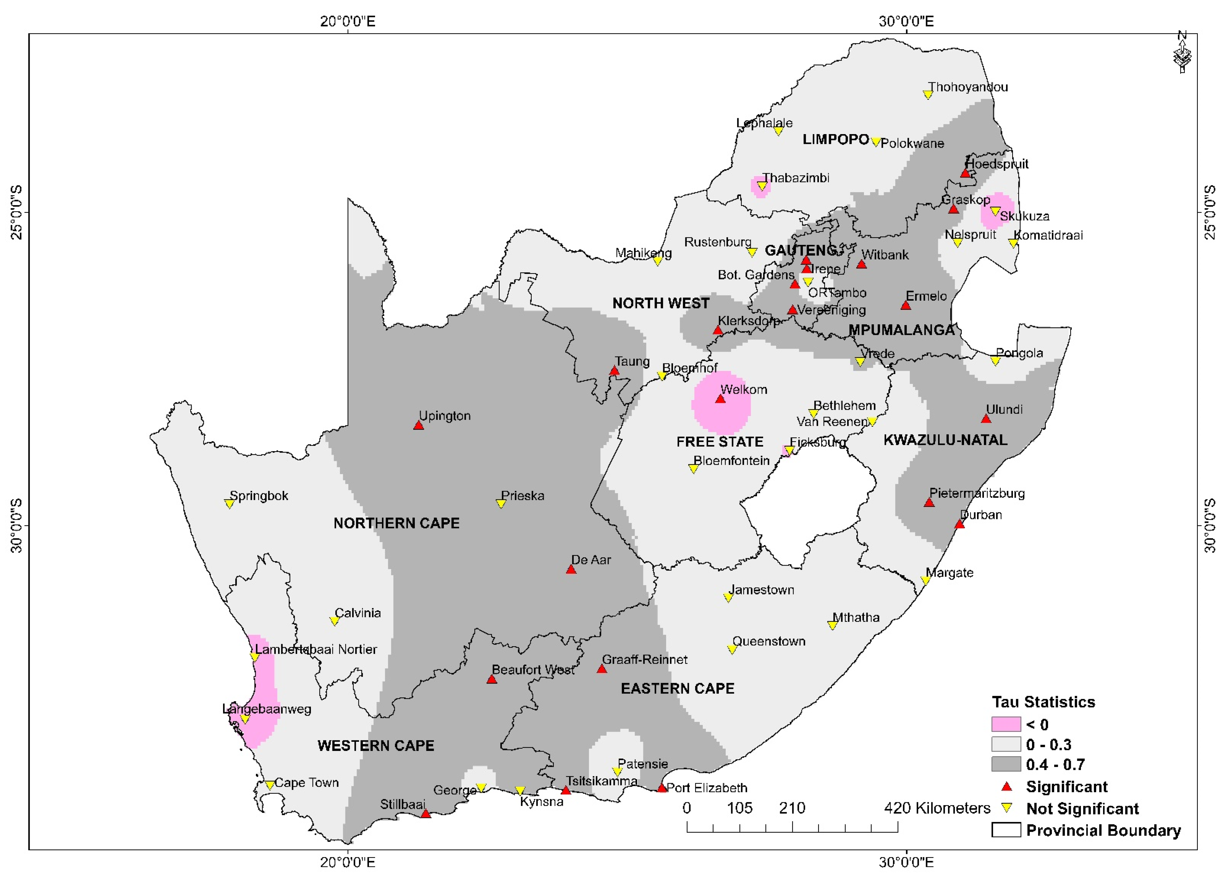
In line with the study by Orimoloye et al. [44], this study investigated trends in AT. However, 23 years of trend analysis might not provide meaningful results (e.g., 30 years). There were increasing trends detected in almost all the weather stations (88%) across the nine provinces, with most of the observed positive trends (47%) being statistically significant at 5% statistical level. The results are consistent with observations of significantly greater warming in the western region and towards the northeastern and eastern parts of South Africa, as per Kruger and Shongwe [41]. Heat stress is expected to become more common and severe due to climate change on a global scale [33]; similar observations have been made for several African countries, including South Africa, Sahelian Africa, and the Northern and Central African countries [43,86], where extreme heat has become an increasing threat to human life. Immediate interventions to mitigate the adverse effects of heat stress and increase the resiliency of affected communities are therefore required.

5. Conclusions

In this research study, 23 years (e.g., 1997–2020) of meteorological data from 51 AWS distributed across South Africa were used to characterize heat stress conditions, thereby identifying the most vulnerable geographical areas that are exposed in the country. The results suggest that low altitude regions, particularly those along the coastlines, are more susceptible to heat stress, with certain localities identified as heat stress hotspots. These include areas in the Cape provinces (EC, NC, and WC) as well as the MP, KZN, and LP provinces. The elevated AT values observed indicate that residents of these regions are most likely to suffer from heat-related diseases such as heat exhaustion, heat cramps, and heatstroke and may even die in severe instances. With exceptions to some pocket areas in the FS, WC, MP, and LP provinces, positive and yet statistically significant trends at 5% significant level were observed across the country, indicating that heat stress has increased in South Africa during the considered study period. To intensify public resilience to heat stress, there is a need to enhance public health surveillance and awareness of the dangers of heat stress locally. Additionally, to address a noted shortcoming of this study, further research into the direct connections between heat stress and health outcomes based on epidemiological analysis not included in this current heat stress assessment is recommended. Lastly, further studies at the district level that will conduct vulnerability assessments and investigate other driving factors of heat stress such as humidity are recommended. The results presented in this study are essential, as they contribute towards improved decision-making, i.e., initiatives that support the use and mobilization of limited resources required to develop and implement appropriate intervention measures to reduce the risk of heat-related morbidity and mortality in vulnerable areas. In particular, the current findings contribute to the implementation and adaptation policies, which are frequently updated in response to the changing climate.

References

1. Luber, G.; McGeehin, M. Climate change and extreme heat events. Am. J. Prev. Med. 2008, 35, 429–435. [Google Scholar] [CrossRef] [PubMed]
2. Lundgren, K.; Kuklane, K.; Gao, C.; Holmér, I. Effects of heat stress on working populations when facing climate change. Ind. Health 2013, 51, 3–15. [Google Scholar] [CrossRef] [PubMed] [Green Version]
3. Semenza, J.C. Climate change and human health. Int. J. Environ. Res. Public Health 2014, 11, 7347–7353. [Google Scholar] [CrossRef] [PubMed] [Green Version]
4. Abdel-Ghany, A.M.; Al-Helal, I.M.; Shady, M.R. Human thermal comfort and heat stress in an outdoor urban arid environment: A case study. Adv. Meteorol. 2013, 28, 693541. [Google Scholar] [CrossRef] [Green Version]
5. Kampmann, D.F.; Bröde, B.P. Physiological responses to temperature and humidity compared to the assessment by UTCI. Int. Biometeorol. 2012, 56, 505–513. [Google Scholar] [CrossRef]
6. James, A.D.; Christian, K. An assessment of thermal comfort in a warm and humid school building at Accra, Ghana. Adv. Appl. Sci. Res. 2012, 3, 535–547. [Google Scholar]
7. Opitz-Stapleton, S.; Sabbag, L.; Hawley, K.; Tran, P.; Hoang, L.; Nguyen, P.H. Heat index trends and climate change implications for occupational heat exposure in Da Nang, Vietnam. Clim. Serv. 2016, 2-3, 41–51. [Google Scholar] [CrossRef] [Green Version]
8. Rother, H.A.; John, J.; Wright, C.Y.; Irlam, J.; Oosthuizen, R.; Garland, R.M. Perceptions of occupational heat, sun exposure, and health risk prevention: A qualitative study of forestry workers in South Africa. Atmosphere. 2019, 11, 37. [Google Scholar] [CrossRef] [Green Version]
9. Morrison, S.A.; Sims, S.T. Thermoregulation in children: Exercise, heat stress & fluid balance. Ann. Kinesiol. 2014, 5, 41–55. [Google Scholar]
10. Scovronick, N.; Lloyd, S.J.; Kovats, R.S. Climate and health in informal urban settlements. Environ. Urban. 2015, 27, 657–678. [Google Scholar] [CrossRef]
11. Casa, D.J.; DeMartini, J.K.; Bergeron, M.F.; Csillan, D.; Eichner, E.R.; Lopez, R.M.; Ferrara, M.S.; Miller, K.C.; O’Connor, F.; Sawka, M.N.; et al. National athletic trainers’ association position statement: Exertional heat illnesses. J. Athl. Train. 2015, 50, 986–1000. [Google Scholar] [CrossRef] [PubMed] [Green Version]
12. Ramphal-Naley, L. Screening for heat stress in workers and athletes. Baylor Univ. Med. Cent. Proc. 2012, 25, 224–228. [Google Scholar] [CrossRef] [PubMed] [Green Version]
13. Moonen, P.; Defraeye, T.; Dorer, V.; Blocken, B.; Carmeliet, J. Urban physics: Effect of the micro-climate on comfort, health and energy demand. Front. Archit. Res. 2012, 1, 197–228. [Google Scholar] [CrossRef] [Green Version]
14. Busato, F.; Lazzarin, R.M.; Noro, M. Three years of study of the Urban Heat Island in Padua: Experimental results. Sustain. Cities Soc. 2014, 10, 251–258. [Google Scholar] [CrossRef]
15. Luo, M.; Lau, N.C. Increasing heat stress in urban areas of Eastern China: Acceleration by urbanization. Geophys. Res. Lett. 2018, 45, 13060–13069. [Google Scholar] [CrossRef]
16. Takane, Y.; Ohashi, Y.; Grimmond, C.S.B.; Hara, M.; Kikegawa, Y. Asian megacity heat stress under future climate scenarios: Impact of air-conditioning feedback. Environ. Res. Commun. 2020, 2, 015004. [Google Scholar] [CrossRef]
17. Wouters, H.; de Ridder, K.; Poelmans, L.; Willems, P.; Brouwers, J.; Hosseinzadehtalaei, P.; Tabari, H.; Broucke, S.V.; van Lipzig, N.P.M.; Demuzere, M. Heat stress increase under climate change twice as large in cities as in rural areas: A study for a densely populated midlatitude maritime region. Geophys. Res. Lett. 2017, 44, 8997–9007. [Google Scholar] [CrossRef] [Green Version]
18. Schuster, C.; Honold, J.; Lauf, S.; Lakes, T. Urban heat stress: Novel survey suggests health and fitness as future avenue for research and adaptation strategies. Environ. Res. Lett. 2017, 12, 044021. [Google Scholar] [CrossRef]
19. Grubenhoff, J.A.; du Ford, K.; Roosevelt, G.E. Heat-related illness. Clin. Pediatr. Emerg. Med. 2007, 8, 59–64. [Google Scholar] [CrossRef]
20. King, B.; Crews, K.A. Ecologies and Politics of Health, 1st ed.; Routlege: London, UK, 2013; pp. 1–298. [Google Scholar] [CrossRef]
21. Takaro, T.K.; Henderson, S.B. Climate change and the new normal for cardiorespiratory disease. Can. Respir. J. 2015, 22, 52–54. [Google Scholar] [CrossRef]
22. Wang, Y.C.; Lin, Y.K. Association between temperature and emergency room visits for cardiorespiratory diseases, metabolic syndrome-related diseases, and accidents in metropolitan Taipei. PLoS ONE 2014, 9, e99599. [Google Scholar] [CrossRef] [Green Version]
23. Kenny, G.P.; Yardley, J.; Brown, C.; Sigal, R.J.; Jay, O. Heat stress in older individuals and patients with common chronic diseases. Cmaj 2010, 182, 1053–1060. [Google Scholar] [CrossRef] [PubMed] [Green Version]
24. Zhang, Y.; Li, C.; Feng, R.; Zhu, Y.; Wu, K.; Tan, X.; Ma, L. The short-term effect of ambient temperature on mortality in Wuhan, China: A time-series study using a distributed lag non-linear model. Int. J. Environ. Res. Public Health 2016, 13, 722. [Google Scholar] [CrossRef] [PubMed] [Green Version]
25. Paravantis, J.; Santamouris, M.; Cartalis, C.; Efthymiou, C.; Kontoulis, N. Mortality associated with high ambient temperatures, heatwaves, and the urban heat island in Athens, Greece. Sustainability 2017, 9, 606. [Google Scholar] [CrossRef] [Green Version]
26. Tong, S.; Wang, X.Y.; Guo, Y. Assessing the short-term effects of heatwaves on mortality and morbidity in Brisbane, Australia: Comparison of case-crossover and time series analyses. PLoS ONE 2012, 7, e37500. [Google Scholar] [CrossRef] [PubMed] [Green Version]
27. Russo, S.; Sillmann, J.; Fischer, E.M. Top ten European heatwaves since 1950 and their occurrence in the coming decades. Environ. Res. Lett. 2015, 10, 124003. [Google Scholar] [CrossRef]
28. Garcia-Herrera, R.; Díaz, J.; Trigo, R.M.; Luterbacher, J.; Fischer, E.M. A review of the European summer heat wave of 2003. Crit. Rev. Environ. Sci. Technol. 2010, 40, 267–306. [Google Scholar] [CrossRef]
29. Yin, P.; Chen, R.; Wang, L.; Liu, C.; Niu, Y.; Wang, W.; Jiang, Y.; Liu, Y.; Liu, J.; Qi, J.; et al. The added effects of heatwaves on cause-specific mortality: A nationwide analysis in 272 Chinese cities. Environ. Int. 2018, 121, 898–905. [Google Scholar] [CrossRef]
30. Ma, W.; Zeng, W.; Zhou, M.; Wang, L.; Rutherford, S.; Lin, H.; Liu, T.; Zhang, Y.; Xiao, J.; Zhang, Y.; et al. The short-term effect of heat waves on mortality and its modifiers in China: An analysis from 66 communities. Environ. Int. 2015, 75, 103–109. [Google Scholar] [CrossRef] [PubMed]
31. Rosenthal, J.K.; Kinney, P.L.; Metzger, K.B. Intra-urban vulnerability to heat-related mortality in New York City, 1997–2006. Health Place 2014, 30, 45–60. [Google Scholar] [CrossRef] [Green Version]
32. Campbell, S.; Remenyi, T.A.; White, C.J.; Johnston, F.H. Heatwave and health impact research: A global review. Health Place 2018, 53, 210–218. [Google Scholar] [CrossRef] [PubMed]
33. IPCC. Climate Change 2013: The Physical Science Basis. Contribution of Working Group I to the Fifth Assessment Report of the Intergovernmental Panel on Climate Change; Cambridge University Press: Cambridge, UK; New York, NY, USA, 2013. [Google Scholar] [CrossRef]
34. Peng, R.D.; Bobb, J.F.; Tebaldi, C.; McDaniel, L.; Bell, M.L.; Dominici, F. Toward a quantitative estimate of future heat wave mortality under global climate change. Environ. Health Perspect. 2011, 119, 701–706. [Google Scholar] [CrossRef] [PubMed] [Green Version]
35. Rodrigues, M.; Santana, P.; Rocha, A. Statistical modelling of temperature-attributable deaths in Portuguese metropolitan areas under climate change: Who is at risk? Atmosphere 2020, 11, 159. [Google Scholar] [CrossRef] [Green Version]
36. Kingsley, S.L.; Eliot, M.N.; Gold, J.; Vanderslice, R.R.; Wellenius, G.A. Current and projected heat-related morbidity and mortality in Rhode Island. Environ. Health Perspect. 2016, 124, 460–467. [Google Scholar] [CrossRef] [PubMed] [Green Version]
37. Rai, M.; Breitner, S.; Wolf, K.; Peters, A.; Schneider, A.; Chen, K. Impact of climate and population change on temperature-related mortality burden in Bavaria, Germany. Environ. Res. Lett. 2019, 14, 124080. [Google Scholar] [CrossRef]
38. Ziervogel, G.; New, M.; Archer van Garderen, E.; Midgley, G.; Taylor, A.; Hamann, R.; Stuart-Hill, S.; Myers, J.; Warburton, M. Climate change impacts and adaptation in South Africa. Wiley Interdiscip. Rev. Clim. Chang. 2014, 5, 605–620. [Google Scholar]
39. Engelbrecht, F.; Adegoke, J.; Bopape, M.J.; Naidoo, M.; Garland, R.M.; Thatcher, M.; McGregor, J.; Katzfey, J.; Werner, M.; Ichoku, C.; et al. Projections of rapidly rising surface temperatures over Africa under low mitigation. Environ. Res. Lett. 2015, 10, 085004. [Google Scholar] [CrossRef]
40. Jury, M.R. Climate trends across South Africa since 1980. Water 2018, 44, 297–307. [Google Scholar] [CrossRef] [Green Version]
41. Kruger, A.C.; Shongwe, S. Temperature trends in South Africa: 1960–2003. Int. J. Climatol. 2004, 24, 1929–1945. [Google Scholar] [CrossRef]
42. Collins, J.M. Temperature variability over Africa. J. Clim. 2011, 24, 3649–3666. [Google Scholar] [CrossRef] [Green Version]
43. Garland, R.M.; Matooane, M.; Engelbrecht, F.A.; Bopape, M.J.M.; Landman, W.A.; Naidoo, M.; Merwe, J.V.D.; Wright, C.Y. Regional projections of extreme apparent temperature days in Africa and the related potential risk to human health. Int. J. Environ. Res. Public Health 2015, 12, 12577–12604. [Google Scholar] [CrossRef]
44. Orimoloye, I.R.; Perez, S.P.; Mazinyo, N.W.; Iortyom, E.T. Climate variability and heat stress index have increasing potential ill-health and environmental impacts in East London, South Africa. Int. J. Appl. Eng. Res. 2017, 12, 6910–6918. [Google Scholar]
45. Kapwata, T.; Gebreslasie, M.T.; Mathee, A.; Wright, C.Y. Current and potential future seasonal trends of indoor dwelling temperature and likely health risks in rural Southern Africa. Int. J. Environ. Res. Public Health 2018, 15, 952. [Google Scholar] [CrossRef] [Green Version]
46. Department of Health. National Climate Change & Health Adaptation. Plan 2014–2019; Department of Health: Cape Town, South Africa, 2014. [Google Scholar]
47. Republic of South Africa. National Climate Change Response Whitepaper; Government Printer: Pretoria, South Africa, 2011. Available online: http://www.gov.za/sites/www.gov.za/files/national_climatechange_response_whitepaper_0.pdf (accessed on 11 December 2020).
48. World Health Organization (WHO). EuroHEAT: Improving Public Health Responses to Extreme Weather/Heatwaves. Summary for Policy-Makers; WHO Regional Office for Europe: Copenhagen, Denmark, 2009. [Google Scholar]
49. Berry, P.; Yusa, A.; Morris-Oswald, T.; Rogaeva, A. Heat alert and response systems in urban and rural communities in Canada. Chang. Adapt. Socio Ecol. Syst. 2014, 1, 84–97. [Google Scholar] [CrossRef]
50. Steadman, R.G. A universal scale of apparent temperature. J. Appl. Meteorol. Climatol. 1984, 23, 1674–1687. [Google Scholar] [CrossRef]
51. Encyclopaedia Britannica. An Introduction to South Africa, with a Focus on Its Geography and History. 2020. Available online: https://www.britannica.com/video/136534/introduction-focus-history-South-Africa-geography (accessed on 15 July 2021).
52. Pocket Guide to South Africa. Provinces 2016–2017. Available online: https://www.gcis.gov.za/sites/default/files/pictures/provinces1617.pdf (accessed on 1 August 2021).
53. Statistics South Africa. Library Cataloguing-in-Publication (CIP) Data; 2011 Statistical Release; Statistics South Africa Census: Pretoria, South Africa, 2011. [Google Scholar]
54. Daron, J. Regional Climate Messages for Southern Africa. Scientific Report from the CARIAA Adaptation at Scalein Semi-Arid Regions (ASSAR) Project. 2014. Available online: http://www.assar.uct.ac.za/sites/default/files/image_tool/images/138/RDS_reports/climate_messages/Southern%20Africa%20Climate%20Messages%20-%20Version%201%20-%20Regional%20Level.pdf (accessed on 15 July 2021).
55. Mahlobo, D.; Funde, S.; Phakula, S. Climate Data & SAWS; South African Weather Service: Pretoria, South Africa, 2013. [Google Scholar]
56. Blazejczyk, K.; Epstein, Y.; Jendritzky, G.; Staiger, H.; Tinz, B. Comparison of UTCI to selected thermal indices. Int. J. Biometeorol. 2012, 56, 515–535. [Google Scholar] [CrossRef] [PubMed] [Green Version]
57. Epstein, Y.; Moran, D.S. Thermal comfort and the heat stress indices. Ind. Health 2006, 44, 388–398. [Google Scholar] [CrossRef] [Green Version]
58. Buzan, J.R.; Oleson, K.; Huber, M. Implementation and comparison of a suite of heat stress metrics within the Community Land Model version 4.5. Geosci. Model Dev. 2015, 8, 151–170. [Google Scholar] [CrossRef] [Green Version]
59. Masterton, J.M.; Richardson, F.A. HUMIDEX, A Method of Quantifying Human Discomfort Due to Excessive Heat and Humidity, CLI 1–79; Environment Canada, Atmospheric Environment Service: Downsview, ON, Canada, 1979. [Google Scholar]
60. NOAA. Heat Stress Index. Available online: http://www.nws.noaa.gov/om/heat/heat_index.shtml (accessed on 15 July 2021).
61. Keone, H.D. An Introduction to Statistics; CreateSpace Independent Publishing Platform: Scotts Vally, CA, USA, 2014. [Google Scholar]
62. Brown, J.D.P. Skewness and kurtosis. Shiken JALT Test. Eval. SIG Newsl. 1997, 1, 20–23. [Google Scholar]
63. Plichta, S.B.; Kelvin, E.A. Munro’s Statistical Methods for Health Care Research, 6th ed.; Wolters Kluwer/Lippincott Williams & Wilkins: Philadelphia, PA, USA, 2013. [Google Scholar]
64. Galip, A. A Simple Class of Measures of Skewness; MPRA Paper 72353; University Library of Munich: Munich, Germany, 2016. [Google Scholar]
65. Hahs-Vaughn, D.; Lomax, R. An Introduction to Statistical Concepts, 3rd ed.; Routledge: New York, NY, USA, 2012. [Google Scholar] [CrossRef]
66. DeCarlo, L.T. On the meaning and use of kurtosis. Psychol. Methods 1997, 2, 292–307. [Google Scholar] [CrossRef]
67. Mann, H.B. Non-parametric tests against trend. Econometrica 1945, 13, 245–259. [Google Scholar] [CrossRef]
68. Kendall, M.G. Rank Correlation Measure; Griffin: London, UK, 1975. [Google Scholar]
69. Theil, H. A Rank-Invariant Method of Linear and Polynomial Regression Analysis; Springer: Amsterdam, The Netherlands, 1950; pp. 345–381. [Google Scholar]
70. Sen, P.K. Estimates of the regression coefficient based on Kendall’s tau. J. Am. Stat. Assoc. 1968, 63, 1379–1389. [Google Scholar] [CrossRef]
71. Malik, A.; Kumar, A. Spatio-temporal trend analysis of rainfall using parametric and non-parametric tests: Case study in Uttarakhand, India. Theor. Appl. Climatol. 2020, 140, 183–207. [Google Scholar] [CrossRef]
72. Babak, O.; Deutsch, C.V. Statistical approach to inverse distance interpolation. Stoch. Environ. Res. Risk Assess. 2009, 23, 543–553. [Google Scholar] [CrossRef]
73. Liu, Z.; Zhang, Z.; Zhou, C.; Ming, W.; Du, Z. An adaptive inverse-distance weighting interpolation method considering spatial differentiation in 3D geological modeling. Geosciences 2021, 11, 51. [Google Scholar] [CrossRef]
74. Lu, G.Y.; Wong, D.W. An adaptive inverse-distance weighting spatial interpolation technique. Comput. Geosci. 2008, 34, 1044–1055. [Google Scholar] [CrossRef]
75. Crider, K.G.; Maples, E.H.; Gohlke, J.M. Incorporating occupational risk in heat stress vulnerability mapping. J. Environ. Health 2014, 77, 16–22. [Google Scholar]
76. Baccini, M.; Biggeri, A.; Accetta, G.; Kosatsky, T.; Katsouyanni, K.; Analitis, A.; Anderson, H.R.; Bisanti, L.; D’Ippoliti, D.; Danova, J.; et al. Heat effects on mortality in 15 European cities. Epidemiology 2008, 19, 711–719. [Google Scholar] [CrossRef] [PubMed]
77. Almeida, S.P.; Casimiro, E.; Calheiros, J. Effects of apparent temperature on daily mortality in Lisbon and Oporto, Portugal. Environ. Health A Glob. Access Sci. Source 2010, 9, 12. [Google Scholar] [CrossRef] [Green Version]
78. Wichmann, J. Heat effects of ambient apparent temperature on all-cause mortality in Cape Town, Durban and Johannesburg, South Africa: 2006–2010. Sci. Total Environ. 2017, 587–588, 266–272. [Google Scholar] [CrossRef] [Green Version]
79. Azongo, D.K.; Awine, T.; Wak, G.; Binka, F.N.; Oduro, A.R. A timeseries analysis of weather variability and all-cause mortality in the Kasena-Nankana Districts of Northern Ghana, 1995–2010. Glob. Health Action 2012, 5, 14–22. [Google Scholar] [CrossRef] [PubMed] [Green Version]
80. Egondi, T.; Kyobutangi, C.; Kovats, S.; Muindi, K.; Ettarh, R.; Rocklov, J. Time-series analysis of weather and mortality patters in Nairobi’s informal settlements. Glob. Health Action 2012, 5, 23–32. [Google Scholar] [CrossRef] [PubMed]
81. Statistics South Africa. Report-03-01-60—Census 2011: Profile of Older Persons in South Africa; Statistics South Africa: Pretoria, South Africa, 2014. [Google Scholar]
82. Statistics South Africa. Midyear Population Estimates; Statistics South Africa: Pretoria, South Africa, 2017. [Google Scholar]
83. Weimann, A.; Oni, T. A systematized review of the health impact of urban informal settlements and implications for upgrading interventions in South Africa, a rapidly urbanizing middle-income country. Int. J. Environ. Res. Public Health 2019, 16, 3608. [Google Scholar] [CrossRef] [PubMed] [Green Version]
84. Baffi, S.; Turok, I.; Vacchiani-Marcuzzo, C. The South African Urban System. In International and Transnational Perspectives on Urban Systems; Rozenblat, C., Pumain, D., Velasquez, E., Eds.; International and Transnational Perspectives on Urban Systems; Springer: Singapore, 2018; pp. 258–314. [Google Scholar]
85. Tran, K.; Azhar, G.; Nair, R.; Dileep, M.; Jaiswal, A.; Knowlton, K.; Hess, J. Assessing Vulnerability to Extreme Heat Among Residents of Urban Slums in Ahmedabad, India; Emory University: Atlanta, GA, USA, 2012. [Google Scholar]
86. Sylla, M.B.; Faye, A.; Giorgi, F.; Diedhiou, A.; Kunstmann, H. Projected heat stress under 1.5 °C and 2 °C global warming scenarios creates unprecedented discomfort for humans in West Africa. Earth’s Future 2018, 6, 1029–1044. [Google Scholar] [CrossRef]
Figure 1. Distribution of observational sites used in this study. The red diamonds in the figure indicate the location of the weather stations in each province.
Sustainability 13 13249 g001
Figure 2. Annual median Apparent Temperature (ATmed) across 51 selected stations.
Sustainability 13 13249 g002
Figure 3. Probability distribution for the different exposure categories across the 51 stations. (a) annual extreme danger, (b) annual danger, (c) annual extreme caution and (d) annual caution.
Sustainability 13 13249 g003aSustainability 13 13249 g003bSustainability 13 13249 g003c
Figure 4. The spatial distribution of Mann–Kendall trend test across the 51 weather stations.
Sustainability 13 13249 g004
Figure 5. The spatial distribution of the Z-score and Theil–Sen slope across the 51 weather stations.
Sustainability 13 13249 g005
Figure 6. Coefficient of Variation of AT, spatially represented.
Sustainability 13 13249 g006
Figure 7. Skewness and Kurtosis Statistics of AT.
Sustainability 13 13249 g007