Article

Study on the Geological Condition Analysis and Grade Division of High Altitude and Cold Stope Slope

1
School of Resources, Environment and Materials, Guangxi University, Nanning 530004, China
2
School of Environment and Resources, Xiangtan University, Xiangtan 411105, China
*
Authors to whom correspondence should be addressed.
Sustainability 2021, 13(22), 12464; https://doi.org/10.3390/su132212464
Submission received: 2 October 2021 / Revised: 7 November 2021 / Accepted: 7 November 2021 / Published: 11 November 2021
(This article belongs to the Special Issue Advances in Rock Mechanics and Geotechnical Engineering)

Abstract

:
Analysis of the geological conditions of high-altitude and low-temperature stope slopes and the study of grade division are the basis for the evaluation of slope stability. Based on the engineering background of the eastern slope of the Preparatory iron mine in Hejing County, Xinjiang, we comprehensively analyse and summarize the factors that affect the geological conditions of high-altitude and cold slopes and finally determine nine geological conditions that affect the index parameters. Based on a back-propagation (BP) neural network algorithm, we establish an applicable network model to analyse the geological conditions of slopes in cold areas. The model is applied to the eastern slope to analyse and classify the geological conditions of the high-altitude and low-temperature slopes. The research results show that the skarn rock layer in the eastern slope is in a stable state and not prone to landslides, and its corresponding geological condition is Grade I; meanwhile, the monzonite porphyry rock layer is in a relatively stable state, with a potential for landslides and a corresponding geological condition Grade II. The marble rock layer is in a generally stable state, there is the possibility of landslide accidents, and the corresponding geological condition level is Grade III. The limestone rock layer is in an unstable state and prone to landslide accidents, it has a corresponding geology condition Grade IV. Therefore, the eastern slope can be divided into different geological condition regions: Zone I, Zone II, Zone III, and Zone IV, and the corresponding geological condition levels for these are Grade I, Grade II, Grade III, and Grade IV. These results may provide a basis for the stability evaluation of high altitudes and cold slopes.

1. Introduction

Slope instability is one of the world’s geological disasters [1,2,3,4]. Every year, the economic losses of various countries in the world caused by geological disasters due to slope instability reach immeasurable levels [5,6,7]. Currently, there are no accurate statistics on the loss, but the loss is still huge. Under the action of freezing and thawing cycles, blasting mining, weathering and other factors, slopes in cold areas can easily cause damage to the mechanical properties of rock slopes and lead to their instability in mines in cold areas [8,9,10,11]. Therefore, open pit mine slope landslides are a potential hazard in harsh environments with high altitudes and cold areas. For example, the “329” landslide disaster. On 29 March 2013, a landslide occurred on Zeri Mountain in the Jiama (in Tibet Province) mining area of the China National Gold Group, causing more than 2 million cubic metres of slope landslides. Eighty-three field workers were buried, and the landslide was investigated afterwards. The reason was found to be factors such as the freezing and thawing of ice and snow.
With the implementation of Western development and progress of engineering technology, difficult-to-mine mineral resources and hidden dangers left over by exploited mineral resources in the harsh environments of Tibet, Xinjiang and other cold regions have begun to receive national attention. The stability of the geological conditions of stope slopes directly affect the smooth development of the mine. Therefore, it is very important to effectively analyse the geological conditions of stope slopes.
The analysis and classification of slope geological conditions can provide an important basis to formulate disaster prevention and mitigation measures and have guiding significance for landslide disaster mitigation planning [12]. Based on the engineering background of the eastern slope of the Preparatory iron mine in Hejing County, Xinjiang, this paper comprehensively analyses and summarizes the factors that affect the geological conditions of high-altitude and cold slopes and finally determines nine geological conditions that affect the index parameters [5,7,13,14,15,16]. Based on a back-propagation (BP) neural network algorithm, a network mode is established that is suitable for the analysis of the geological conditions of slopes in cold areas. This model is applied to the east slope to analyse and classify the geological conditions of high-altitude and low-temperature slopes.

2. BP Neural Network

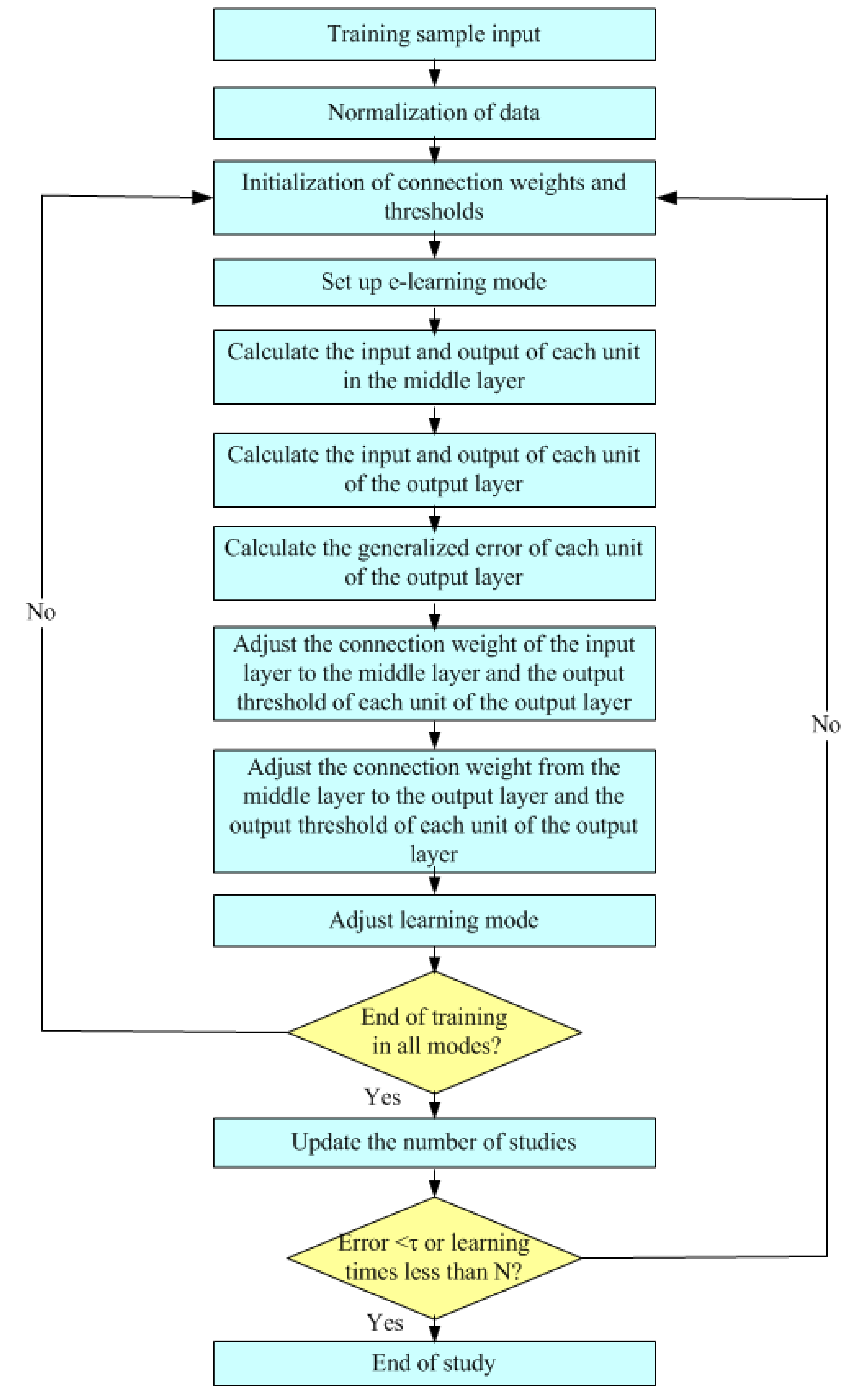
2.1. BP Neural Network Operation Mechanism

In the early 1980s, the theory and research of artificial neural networks (ANNs) made considerable progress under the influence of the sound and continuous development of computers and the continuous breaking of new technical barriers. The theory of artificial neural networks sprouted during this golden period [17] and flourished as a new research paradigm.
Many studies [18,19] have shown that the efficiency of traditional system theory analysis methods is low, and the scientific nature is slightly lacking. Compared with the traditional system theory analysis method, the analysis method of the BP neural network (back-propagation neural network) is more scientific and efficient, the result is more accurate and can convince most researchers in the process of practical application. Compared with the traditional system theory analysis method, it obviously shows stronger competitiveness.
In addition, many studies [20] have found that the adaptive and self-learning capabilities of a BP neural network are outstanding, and the linear function mapping and nonlinear function mapping problems based on a BP neural network are easier to identify for mining systems.
These reasons have made many researchers in the current scientific research field strongly affirm BP neural networks. A BP neural network is a multi-layer feedforward neural network that must reduce the error between the network output and the actual value to a certain range through repeated training and learning so that the network output can reach the required accuracy. A BP neural network method to reduce the error between the network output result and the actual value trains the propagation algorithm according to the forwards multi-layer network structure and reverse feedback. The flow chart of the learning process of a BP neural network is shown in Figure 1.

2.2. Data Processing

This article uses a BP neural network-supervised algorithm to classify the data. The specific method is as follows: by continuously selecting certain characteristic parameters from the sample data that have been collected, trained, checked, filtered, and subsequently set according to the classifier in advance we can determine the criteria and summarize and sort the samples that have been further screened out and have been identified.
Before the data classification process begins, a certain amount of training data must be mastered because the continuous and stable operation of the BP neural network strictly requires the input of relevant training data. Only in this way can it be extracted through the feature extraction of the input training data in the subsequent classification process to establish a scientific and rigorous classification model. Then, the existing training data are analysed by comparing the classification model with the verification model. Finally, the classification of the data is completed.
To eliminate the influence of other transformation functions on the transformed image as much as possible, it is necessary to normalize the collected data. Normalization processing refers to the use of the principle of invariant moments to convert the unquantifiable expression form into a value in the range of 0–1 for processing so that the expression form becomes a scalar.
The formula for data normalization is:
y = x M i n v a l u e M a x v a l u e M i n v a l u e
where x is the value before conversion, y is the converted value, M i n v a l u e is the sample minimum and M a x v a l u e is the sample maximum.
The BP neural network actually achieves the accuracy requirements through repeated training of multiple samples to find the minimum value of the error function. The most common method to determine whether the error satisfies the error accuracy requirement is logistic regression. This article uses a binary logistic regression method to determine the two results (True/False) of the input data and the corresponding probability (PTrue/PFalse) of the results to determine whether the accuracy of the network system satisfies the requirements. The formula is as follows:
t = w x + b
In the formula:
x—input sample parameters;
t—temporary variable;
w, b—model parameters.
The sigmoid function is usually used as the use condition of the conversion function: in the logical judgment, when h(t) > 0.5, y = 1. The formula is as follows:
h ( t ) = 1 1 e t
From formula (3), we can see: its parameter curve is shown in Figure 2.

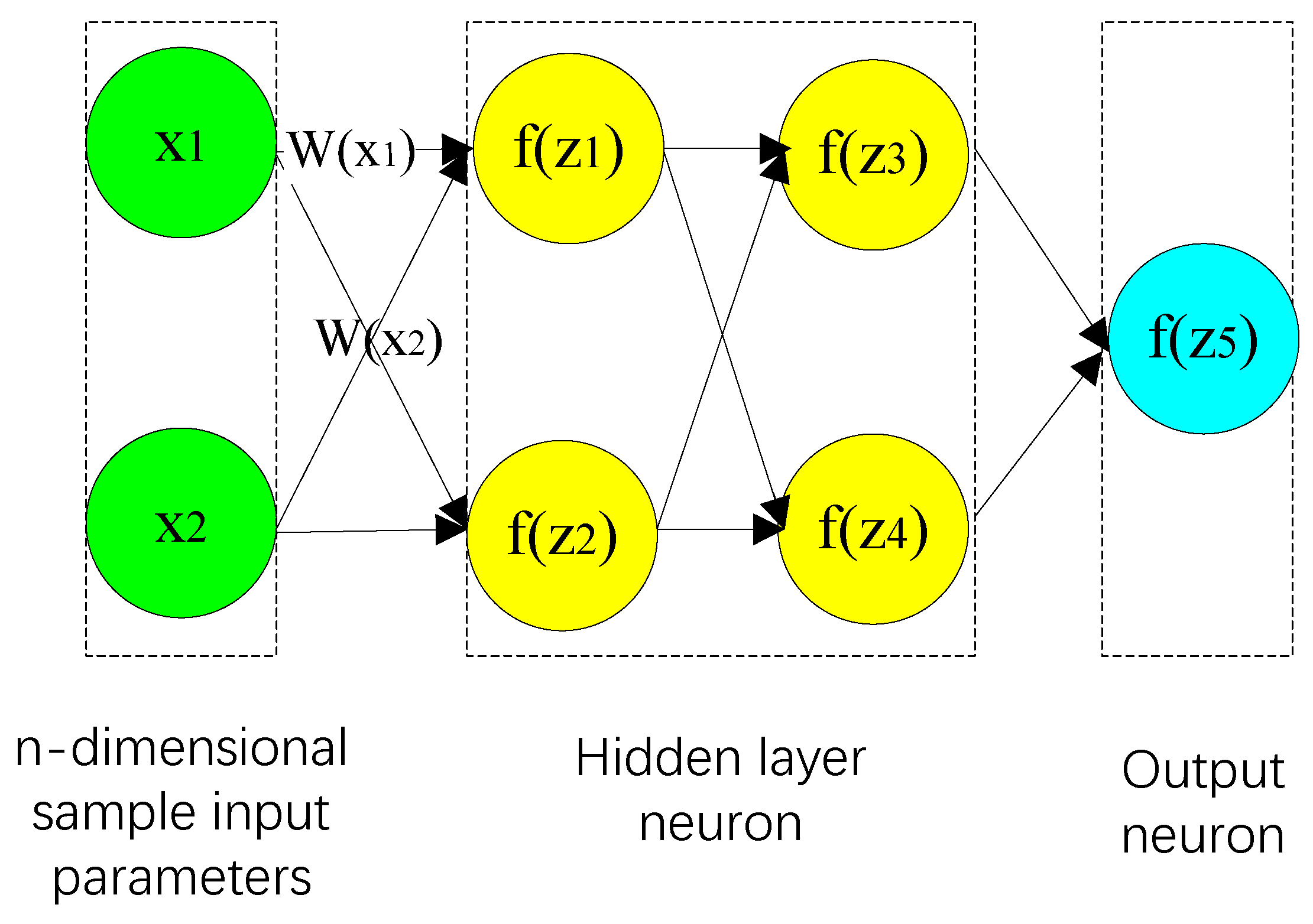
2.3. BP Neural Network Forward Transmission and Reverse Feedback

(1) Forward transmission
The input parameters of the neural network reach the output end through the input end and each node of the intermediate layer (hidden layer). This method is forward transmission. The intermediate layer can be adjusted by changing the weight relationship between the intermediate layer and the output layer, output threshold updating of the intermediate layer, and other adjustment methods to reduce the generalization error between each node and the actual value, and to therefore achieve the desired result.
The multi-layer perceptron is composed of one or more single-layer perceptrons, which can calculate nonlinear data. The input and output ends of the multi-layer perceptron contain multiple hidden layers [18]. However, thus far, there are different opinions on the number of hidden layers.
The decision-making area of a single-layer perceptron is divided by an extended two-dimensional data plane. In addition, when the multi-layer perceptron contains only one hidden layer, the decision-making area can be an open convex area or a closed concave area. When the multilayer perceptron contains more than one hidden layer, its decision-making area can show diversified shapes and area divisions. Figure 3 shows the change in the weight relationship during the forward transmission.
Neural network training samples must introduce randomly assigned weights and biases. Simultaneously, the randomly assigned weights and random assigned biases introduced are not randomly selected but must satisfy the weights. The condition of interval real number is (–1, 1), and the offset is (0, 1) interval real number. Only after the abovementioned conditions are satisfied can the network model be forward propagated again. In this process, X1 and X2 are calculated by formulas (4)–(8).
For the neuron ƒ(z1), the following calculations are performed when only the weight assignment is considered:
y 1 = f ( z 1 ) = f ( w ( x 1 ) 1 × x 1 + w ( x 2 ) 1 × x 2 )
In the formula, w ( x 1 ) 1 represents the weight of x 1 to y 1 , as shown in Figure 3. Similarly, we can calculate:
y 2 = f ( z 2 ) = f ( w ( x 2 ) 2 × x 1 + w ( x 2 ) 2 × x 2 )
y 3 = f ( z 3 ) = f ( w ( y 1 ) 1 × y 1 + w ( y 2 ) 1 × y 2 )
y 4 = f ( z 4 ) = f ( w ( y 1 ) 2 × y 1 + w ( y 2 ) 2 × y 2 )
y 5 = f ( z 4 ) = f ( w ( y 3 ) 1 × y 3 + w ( y 4 ) 1 × y 4 )
In summary, the output value of each node can be calculated by the formula of forward transmission. Accordingly, the actual output result of the forward transmission model can also be obtained by calculation, and the final output result y 5 obtained by the above formula is exactly the actual output result of the forward transmission mode.
(2) Back feedback
To facilitate the error to participate in subsequent calculations, this article assumes that t is the expected output value of the training data. Because y 5 is the actual output value of the forward propagation model, it is assumed that the difference between the actual output value and the expected output value is δ = t y 5 . In addition, the difference between the actual output value and the expected output value must be based on actual conditions during the definition process. It is assumed that there is an error between the actual output value and the expected output value of each node, and this error is defined as δi. By training the error between the actual value and the expected value, the adjustment of the weight is a crucial step for the feedback adjustment of the BP neural network. The specific process is shown in Figure 4.
For the error, δ 3 = w ( y 3 ) δ , and similarly,. δ 4 = w ( y 4 ) δ The calculation method for δ 1 and δ 2 is as follows:
δ 1 = w ( y 1 ) 1 δ 3 + w ( y 1 ) 2 δ 4
δ 2 = w ( y 2 ) 1 δ 3 + w ( y 2 ) 2 δ 4
Using formula (9) and calculating according to the principle of this formula, the value of δ 1 , δ 2 , δ 3 , δ 4 can be finally obtained. In addition, the theoretical basis of back propagation is the change in relationship between the error and the weight. The variation Δ w i obtained by adjusting the weight is calculated by error. The calculation formula of the weight variation is as follows:
Δ w i = η δ i d f ( z i ) d z i x i
where: η is the learning rate.
The weight of w ( x 1 ) 1 can be adjusted as follows:
w ( x 1 ) 1 = w ( x 1 ) 1 + η δ i d f ( z i ) d z i x 1
Similarly, the weight of w ( x 2 ) 1 is adjusted as:
w ( x 2 ) 1 = w ( x 2 ) 1 + η δ i d f ( z i ) d z i x 1
The weight is calculated and adjusted according to Formula (12), and the final result is an update of the weight. A single back propagation includes the calculation, adjustment and updating of the weights of all nodes. Only after these tasks are completed is back propagation considered completed once. The essence of the realization of the reverse transmission algorithm is to complete the parameter adjustment of the sample model. In this process, forward transmission and reverse feedback are continuously performed. Finally, the error, weight and accuracy of the model reach the desired value.
In summary, the training process of the neural network can be completed through forward transmission and reverse feedback. However, this type of training will not continue indefinitely. Under certain conditions, the training will stop. The BP network training model stops in two situations; after setting and reaching the maximum number of iterations and after reaching a certain threshold.

3. Construction of a BP Neural Network Suitable for Preparing Iron Ore Slopes

3.1. Geological Condition Analysis and Network Output Parameter Setting

(1) Determine the geological conditions index
In the process of using the BP neural network to classify and predict the geological conditions of the stope slope, it is necessary to establish the corresponding BP neural network model. The first step in establishing a BP neural network model is to evaluate the reliability of its input parameters and filter the parameters to exclude unreliable input parameters so that the final output parameters are as accurate and reliable as possible and can show the influence of different geological factors on the geological conditions of the slope.
Generally, the geological influencing factors of slopes are the slope, slope height, lithology, unit weight, internal friction angle, porosity, cohesion, freeze-thaw cycles, etc. The slope and slope height determine the geometry of the slope and are indispensable factors for its existence. Furthermore, the lithology, gravity, internal friction angle, porosity, cohesion, etc. are important characteristics of the rock mass of the slope as they characterize the quality of the rock mass that composes it. As a unique feature of a slope in a cold region, the freeze-thaw cycle plays a huge role in the classification of geological conditions there. Various geological factors have a certain connection, while some other factors do not. Despite this, all of these factors play a vital role in the division of the slope geological conditions and therefore all will be divided. This is an important factor in the grade of slope geological conditions.
Generally, the number of parameters has little effect on neurons, and the number of parameters only represents the number of input neurons. In addition, the increase in number of parameters increases the simulation recognition time, and the actual engineering volume greatly increases. Therefore, to reduce the actual workload, this paper simplifies the input parameters of the model, and according to the modelling data and simulation results, the slope geological condition indicators are the freeze-thaw coefficient, hydrogeology, rock gravity, cohesion, internal friction angle, slope, slope height, porosity, and other factors.
(2) Set model output parameters
The output parameters are the grades of the geological conditions of the slopes in preparation for the iron ore mine, and the output parameters are divided into 4 grades according to the four expected output values of Grade I, Grade II, Grade III, and Grade IV. The specific content is shown in Table 1.

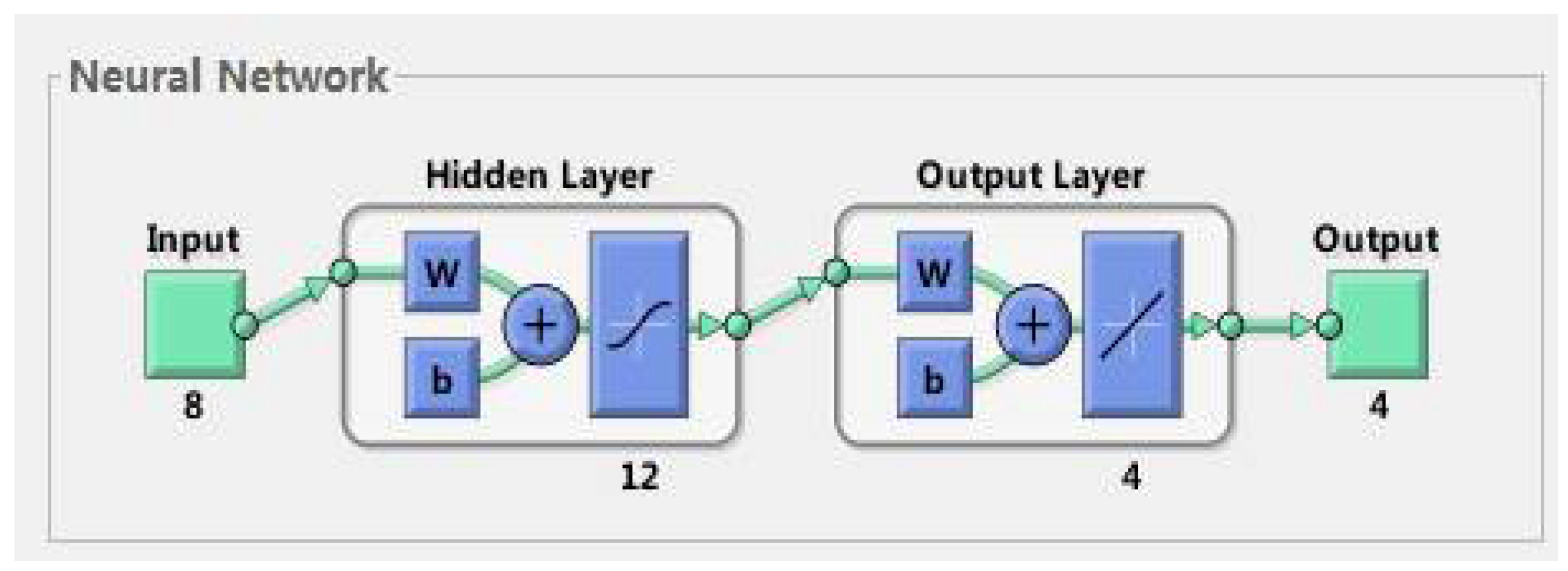
3.2. Determination of the Grid Structure

(1) Determination of the number of perceptrons
The input layer, hidden layer and output layer constitute the basic structure of the BP neural network. The number of hidden layers depends on the complexity of parameter selection. For a more complex problem to be solved, there are more hidden layers, and the difficulty of the corresponding model convergence increases.
(2) Determination of the number of network nodes
The method of dividing the network nodes of the input layer and output layer is unified and clear: generally, once the number of research projects is determined, the input layer and output layer are determined, but there is no scientific and consistent method of dividing the hidden layer of network nodes.
However, the neural network model constructed based on the slope parameters contains only a single hidden layer, so simply calculating the number of nodes in this layer can reveal the number of hidden layer nodes in the entire neural network model, which greatly simplifies the calculation process.
Because the number of rows of the input vector is equal to the number of nodes of the input layer, by knowing that the number of rows of the input vector is 8, it can be directly obtained that the input layer has 8 nodes. In addition, the number of nodes in the output layer is equal to the amount of output data points. Because the number of output data points is 4, it can be concluded that the number of nodes in the output layer is also 4. In addition to the above information and because the number of nodes in the hidden layer is 12, it is finally determined that the structure of the BP neural network is 8-12-4, as shown in Figure 5.

3.3. Selection and Processing of Training Samples

Two key factors of the network model training sample selection are mainly related to the complexity of the training sample. Firstly, the accuracy of the training sample. For training samples, the accuracy is positively correlated with the complexity of the samples. If the accuracy of the training samples increases, the complexity of the samples also increases, which will eventually increase the demand for the number of samples. Secondly, noise in the data. The noise in the sample data is also positively correlated with the complexity of the sample. If the noise in the data increases, the complexity of the training sample will also significantly increase, which affects the selection of the final training sample. Therefore, when training a neural network, it is necessary to control the relationship between the complexity of the sample and the accuracy of the training data and to provide as much key and useful information as possible to reduce the interference of redundant and useless information.
After consulting a large quantity of mine slope data, 54 neural network training samples were selected from them, with the literature [21,22] has mentioning the necessity of checking the dependency of each parameter before the ANN. However, the dependency of the parameters does not need to be discussed in this study. Because all the parameters are randomly selected, there is no dependence between the parameters in the nine main slope-influencing factors (according to the actual situation of Beizhan iron ore). All parameters are shown in Table 2, and the normalized data processing is shown in Table 3.

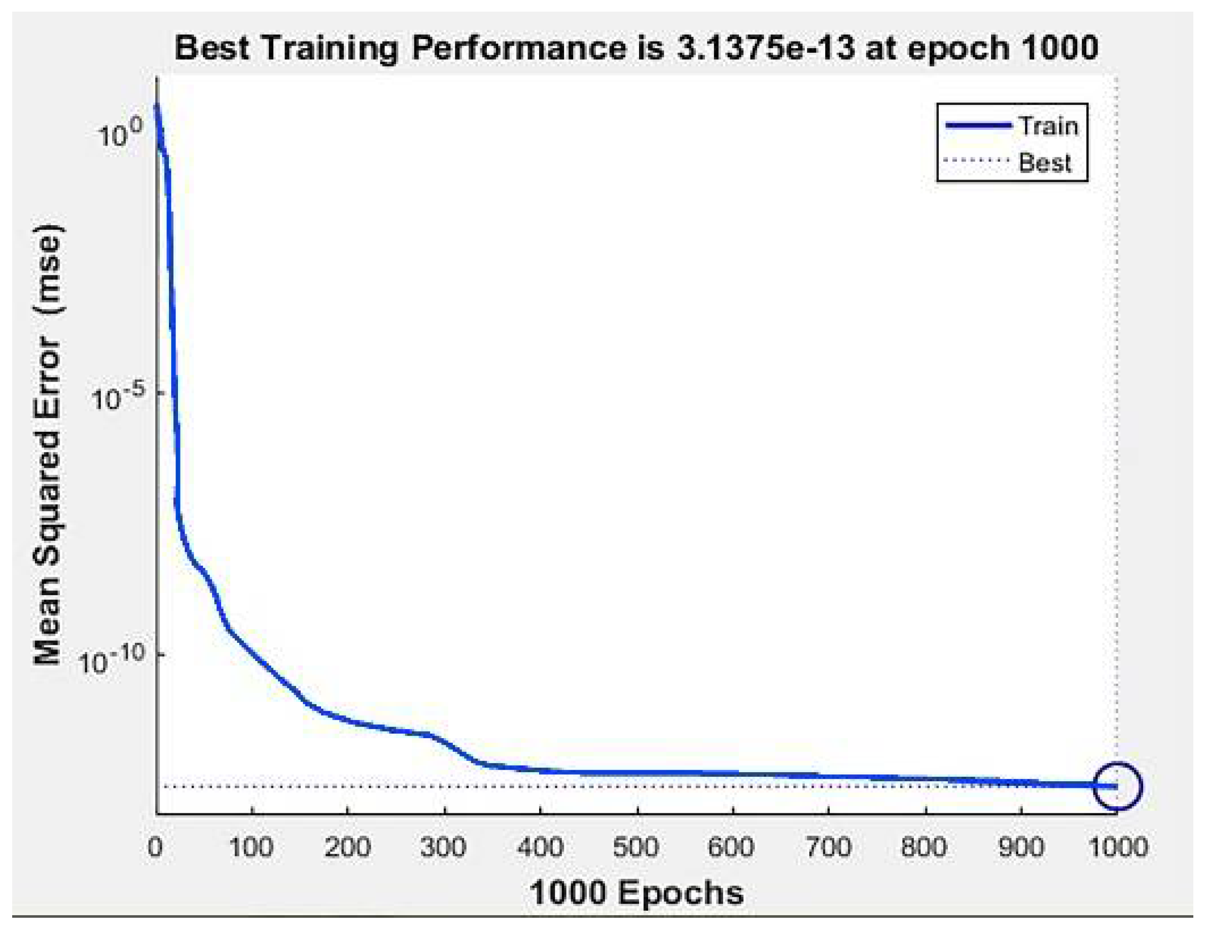
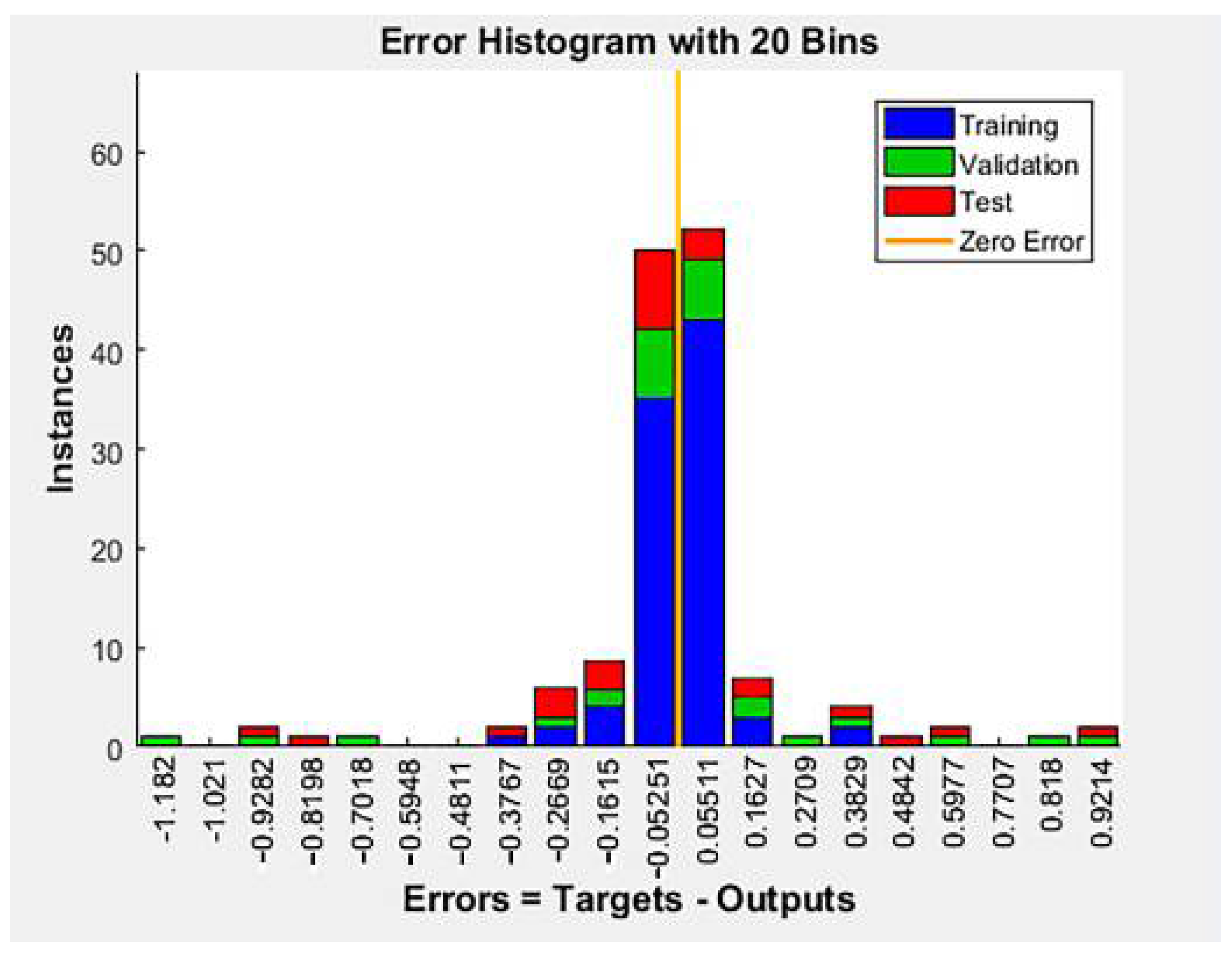
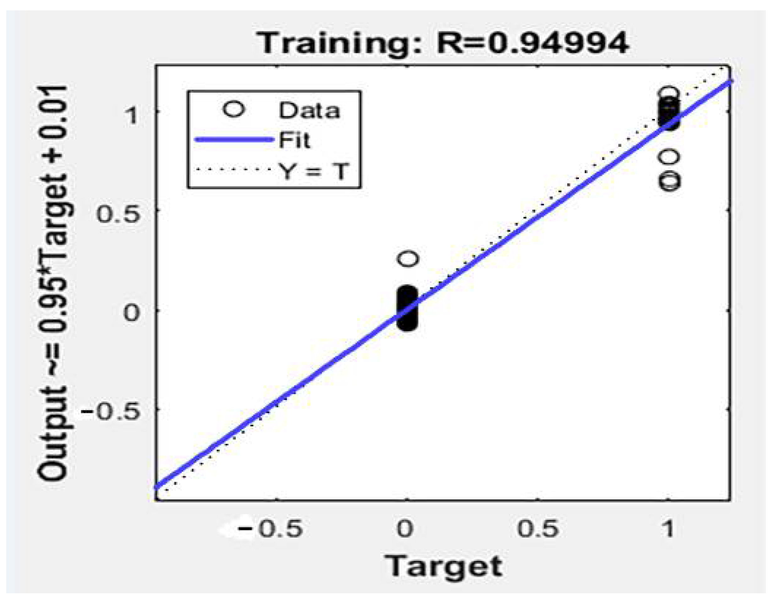
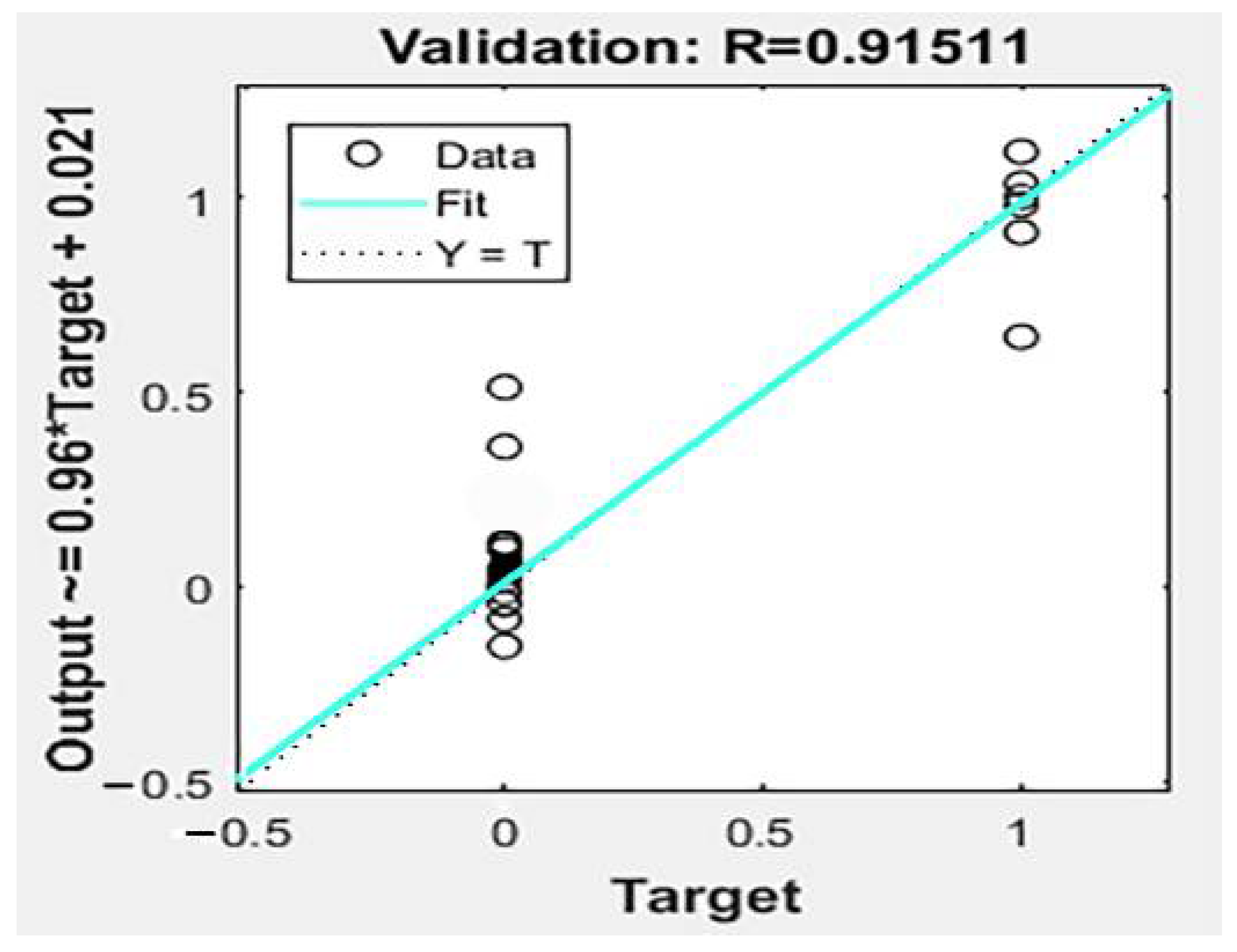
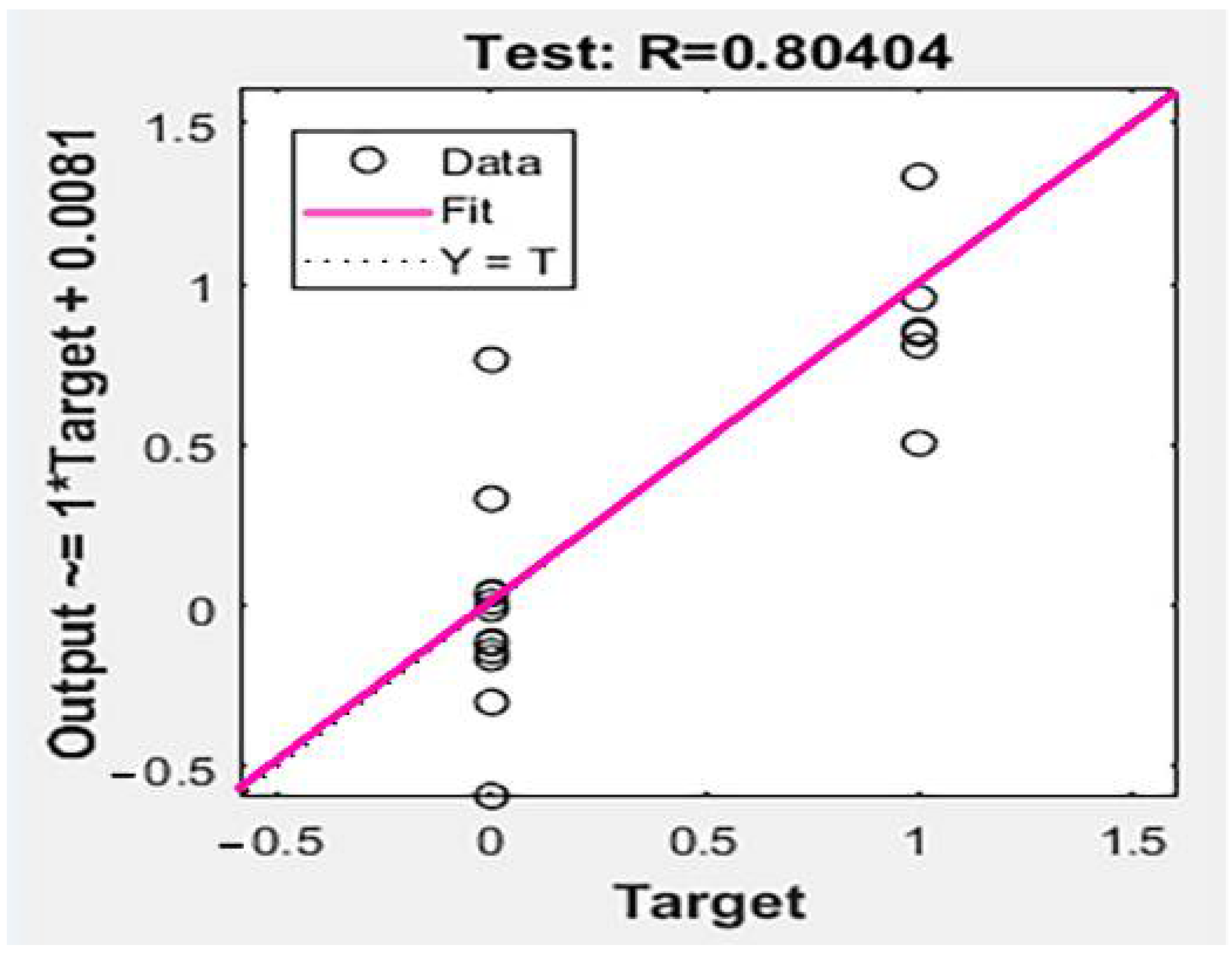
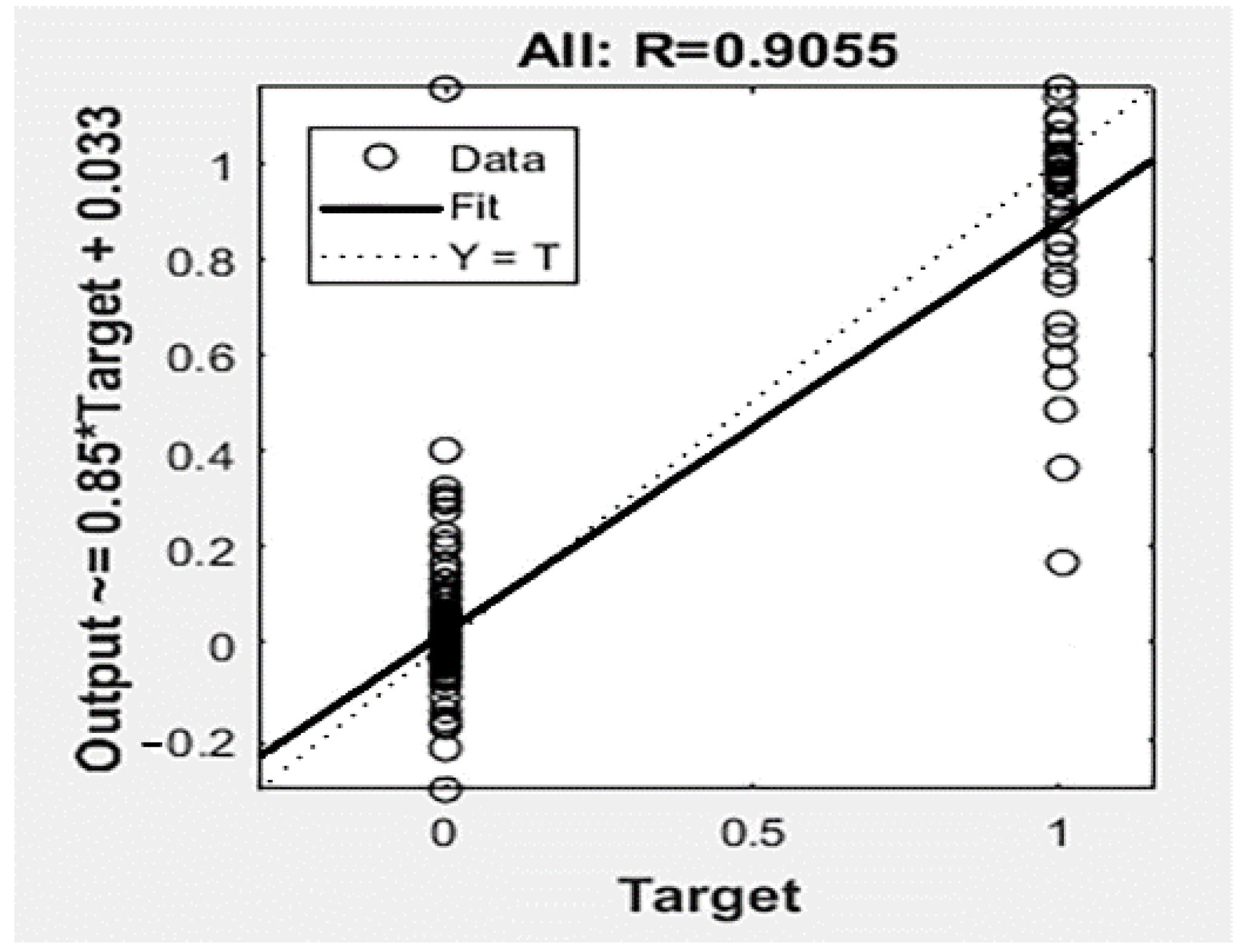
3.4. Sample Training and Result Analysis

The training steps are shown in Figure 6.
(1) Convergence graph
According to the data, the convergence curve is shown in Figure 7, which shows that the minimum momentum is added to the training so that the probability that the convergence curve has a local minimum is reduced after 1000 iterations of learning.
(2) Error distribution diagram
According to the data, the error distribution histogram is shown in Figure 8. The distribution histogram shows that the predicted sample is compared with the actual sample, and the error value is mostly distributed between −6% and 6%, which indicates that the result after training is reliable.
(3) Regression analysis graph
Regression diagrams are made according to the data: Figure 9 shows the regression diagram of 70% training samples; Figure 10 shows the regression diagram of 15% verification samples; Figure 11 shows the regression diagram of 15% test samples; Figure 12 shows the regression diagram of the overall sample. Among them, the abscissas 0 and 1 represent the target value, and the ordinate represents the sample value after debugging. If the slope of the curve approaches 1, it means that the target value is very close to the theoretical value, which implies that the regression analysis is very accurate.
The sample data in Table 4 represent the true value and predicted value of the sample and the error between them. In the table, the error is small (the maximum is 6.1%), which shows that the accuracy of network training is high.

4. Grade Division of Slope Geological Conditions in Preparation for Iron Mines

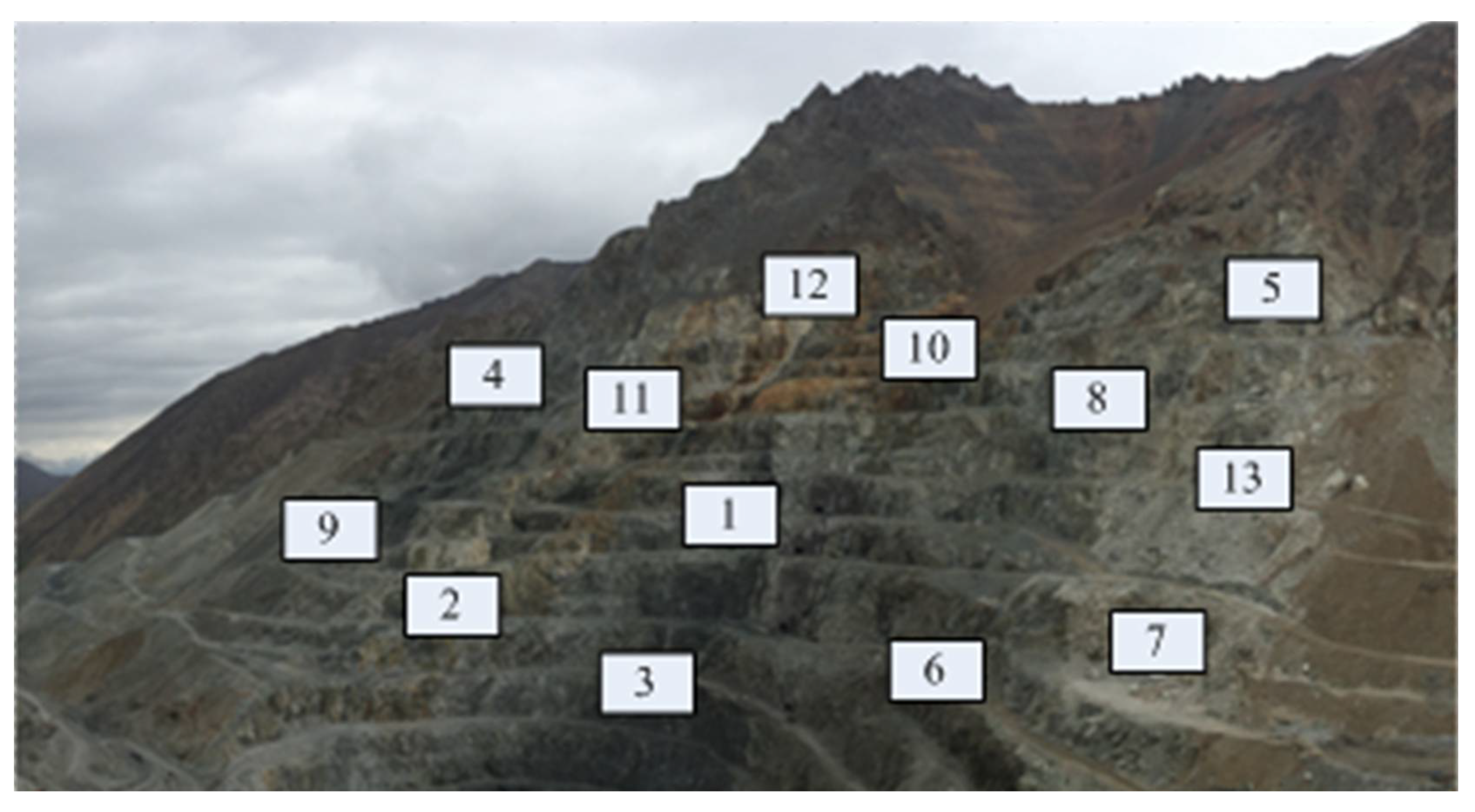
4.1. Determination of Parameter Samples of Geological Condition Indicators

There are two main mining areas in the current mining area of the preparation for iron ore: open-pit mining and side-hanging mining. The slope area of this study is mainly the side slope between the pit and the side-hanging mine, which forms after the open-pit mining, i.e., the east side slope area of the mine. Referring to the geological report of the area and the index data of the test items, a set of parameter samples containing geological conditions index can be obtained, as shown in Table 5.

4.2. Calculation Results and Analysis

According to the training results of the BP neural network model based on the training samples in the previous section, the accuracy of the network is high, so it can be used to prepare for the calculation of the iron ore geological index parameter samples. After normalizing the data in the geological condition parameter table (Table 5), it is input into the neural network model for calculation, and the result is shown in Table 6. Table 7 is obtained after summarizing the samples of the same geological condition level among 13 groups of samples.
Based on Table 7, the BP neural network analysis shows that among the 13 samples of the eastern slope in this cold area, 5 have geological conditions of Grade I, and 3 have geological conditions of Grade II. There are 3 with condition Grade III and 2 with Grade IV conditions. The 13 sample numbers are distributed in different locations on the eastern slope. After their positions have been marked on the eastern slope, the distribution area map of the eastern slope samples, as shown in Figure 13, is obtained.
The numbers 1 to 13 in the diagram are the sampling points, and 13 samples are taken from different areas of the east slope of Beizhan Iron Mine.Figure 13 shows that although the distribution positions of the 13 samples on the eastern slope are random; there is a certain distribution law, i.e., the distribution among the samples at identical or similar geological condition levels is relatively dense, and samples of different geological conditions are far apart and sparsely distributed. As a result, the regions where samples with identical or similar geological condition levels are located can be statistically divided, so that the eastern slope can be divided into geological conditions. The specific divisions are shown in Figure 14.

5. Concluding Remarks

A BP neural network is used to classify the geological conditions of the eastern slope of the preparatory iron mine and the overall division. The eastern slope of the iron mine preparation is divided into four areas: Zone I, Zone II, Zone III, and Zone IV. The corresponding geological condition grades for zones I to IV are grade I, grade II, grade III, and grade IV, respectively. Among them, the rock formation in Zone I is mainly skarn rock formation, which is also the main occurrence area of ore bodies. It has high unit weight, high hardness, undeveloped rock joints, high integrity, and good physical and mechanical properties, so its geological conditions are good. Damage does not easily occur, and the corresponding geological condition is grade I. The rock formation in Zone II is mainly monzonite porphyry. Compared with skarn its weight and hardness are slightly lower, however, the rock layer is thick and the joints are less developed. Therefore, it has better physical and mechanical properties. The conditions are good, there are only potential destructive factors, and the corresponding geological conditions are grade II. The rock formations in Zone III are mainly marble formations. Compared with skarn and monzonite porphyries, marble is relatively poor in lithology, has low gravity and hardness, and has more joints in the formations. The physical and mechanical properties are poor, but its thickness is large, and the layered distribution slightly compensates for the lack of lithology. Therefore, its geological conditions are general, and there is a possibility of damage. The corresponding geological conditions are grade III. The rock formation in Zone IV is mainly limestone rock. It has the worst lithology among the four rock formations, with low unit weight, low hardness, well-developed joints, and large porosity. After long-term weathering, erosion, and freezing and thawing cycles, its physical properties are destroyed. Therefore, the geological conditions in this area are poor and easily destroyed. The corresponding geological conditions are grade IV.

Author Contributions

The research articles with four authors, the Conceptualization R.Z. and S.W.; methodology, Q.C.; software, S.W; validation, R.Z., S.W and Q.C.; formal analysis, C.X.; investigation, C.X.; resources, Q.C.; data curation, S.W.; writing—original draft preparation, S.W.; writing—review and editing, R.Z.; visualization, C.X.; supervision, Q.C.; project administration, Q.C. All authors have read and agreed to the published version of the manuscript.

Funding

The research was funded by the national key research and development project “Slope instability mechanism and early warning technology of open pit in high altitude and cold area” (No. 2018YFC0808402) and the Hunan Province Science Foundation, grant number 2021JJ30679.

Institutional Review Board Statement

This paper does not involve human or animal studies.

Informed Consent Statement

This paper does not involve human research.

Data Availability Statement

All the data included in this study are available upon request by contact with the corresponding author.

Conflicts of Interest

The authors declare no conflict of interest.

References

  1. Fang, R.K.; Liu, Y.H. Review of regional landslide risk assessment methods based on machine learning. Chin. J. Geol. Hazard Control 2021, 32, 1–5. [Google Scholar]
  2. Feng, T.J. Assessment of the Loss of Ecological Carrying Capacity Caused by Landslide Disasters in the Southeastern Mountainous Area of Jilin Province. Master’s Thesis, Northeast Normal University, Changchun, China, 2016. [Google Scholar]
  3. Shang, G.A. Analysis of dump slope deformation monitoring data based on the re-scaled range analysis method. Opencast Min. Technol. 2018, 33, 64–67. [Google Scholar]
  4. Li, C.H.; Xiao, Y.G. Research status and trend of deformation and failure mechanisms of rock slopes in high altitude and cold areas. Chin. J. Eng. Sci. 2019, 41, 1374–1386. [Google Scholar]
  5. Han, G. Research on the Key Technique of Stability and Safety Control of High Bedding Rock Slope in Open-Pit Mine. Ph.D. Thesis, University of Science and Technology Beijing, Beijing, China, 2017; pp. 57–63. [Google Scholar]
  6. Liu, J. Stability Evaluation of Open-Pit Mine Slope Based on Fuzzy-Random Reliability. Master’s Thesis, Central South University, Changsha, China, 2013; pp. 56–58, 70–72. [Google Scholar]
  7. Luo, X.D. Stability Analysis and Engineering Application of High Slope in Open-Pit Mine in Cold Area, 1st ed.; China Meteorological Press: Beijing, China, 2015; pp. 38–39, 46–48. [Google Scholar]
  8. Chen, Y.C. Preliminary Study on Rock and Soil Slope Stability under the Freez-ing-Thawing Condition. Master’s Thesis, Xi’an Technological University, Xi’an, China, 2006; pp. 7–10, 14–15. [Google Scholar]
  9. Luo, X.D.; Huang, C.L.; Rong, Z.X.; Lv, Q.S. Study of physico-mechanical characteristics of rocks in slope of Mengku iron mine under freezing-thawing cyclic effect. Rock Soil Mech. 2011, 32 (Suppl. S1), 155–159. [Google Scholar]
  10. Deng, H.W.; Tian, W.G.; Zhou, K.P.; Li, J.L. Progress in freezing-thawing rock mechanics from 2001 to 2012. Tech. Rev. 2013, 31, 74–79. [Google Scholar]
  11. Meng, L.L.; Chen, Q.F. Stability analysis of high-altitude and high-cold slopes in preparation for iron mine. Non-Ferr. Met. Min. Part 2020, 72, 5–9. [Google Scholar]
  12. Li, Z.; Nadim, F.; Huang, H.; Uzielli, M.; Lacasse, S. Quantitative vulnerability estimation for scenario-based landslide hazards. Landslides 2010, 7, 125–134. [Google Scholar] [CrossRef]
  13. Zhang, B. Geological Characteristics and Genesis of the Preparatory Iron Deposit in Hejing County, Xinjiang. Master’s Thesis, Chang’an University, Xi’an, China, 2016; pp. 14–15, 64–66. [Google Scholar]
  14. Jordá-Bordehore, L. Application of Q slope to Assess the Stability of Rock Slopes in Madrid Province, Spain. Rock Mech. Rock Eng. 2017, 50, 1947–1957. [Google Scholar] [CrossRef]
  15. Bar, N.; Barton, N. The Q-Slope Method for Rock Slope Engineering. Rock Mech. Rock Eng. 2017, 50, 3307–3322. [Google Scholar] [CrossRef]
  16. Bar, N.; Barton, N. Rock Slope Design using Q-slope and Geophysical Survey Data. Period. Polytech. Civ. Eng. 2018, 62, 893–900. [Google Scholar] [CrossRef]
  17. Niu, P.F.; Zhou, A.H. Stability prediction of rock slopes of Central South Highway based on PCA and BP neural network. J. Inst. Disaster Prev. Sci. Technol. 2020, 22, 10–16. [Google Scholar]
  18. Jiang, J. BP neural Networks for Prediction of Factor of safety of Slope Stability. In Proceedings of the 2011 IEEE 2nd International Conference on Computing, Control and Industrial Engineering, Wuhan, China, 20–21 August 2011; Institute of Electrical and Electronics Engineers Inc.: Piscataway, NJ, USA, 2011; Volume 115, pp. 347–350. [Google Scholar]
  19. Zhao, Y.J.; Zhang, E.L.; Gong, Z.Z. The application of BP neural network in slope stability prediction. West. Explor. Eng. 2014, 26, 23–25. [Google Scholar]
  20. Feng, X.T.; Wang, Y.J. Neural network estimation of slope stability. J. Eng. Geol. 1995, 3, 54–61. [Google Scholar]
  21. Chang, S.K.; Lee, D.H.; Wu, J.H.; Juang, C.H. Rainfall-based criteria for assessing slump rate of mountainous highway slopes: A case study of slopes along Highway 18 in Alishan, Tai-wan. Eng. Geol. 2011, 118, 63–74. [Google Scholar] [CrossRef]
  22. Lin, H.M.; Chang, S.K.; Wu, J.H.; Juang, C.H. Neural network-based model for assessing failure potential of highway slopes in the Alishan, Taiwan Area: Pre- and post-earthquake investigation. Eng. Geol. 2009, 104, 280–289. [Google Scholar] [CrossRef]
Figure 1. BP neural network operation flow chart.
Sustainability 13 12464 g001
Figure 2. The Sigmoid curve.
Sustainability 13 12464 g002
Figure 3. Graph of the weight relation changes.
Sustainability 13 12464 g003
Figure 4. Variation diagram of the error feedback relationship.
Sustainability 13 12464 g004
Figure 5. BP neural network structure diagram.
Sustainability 13 12464 g005
Figure 6. Training step diagram.
Sustainability 13 12464 g006
Figure 7. Convergent plot.
Sustainability 13 12464 g007
Figure 8. Error distribution histogram.
Sustainability 13 12464 g008
Figure 9. Regression diagram of training samples.
Sustainability 13 12464 g009
Figure 10. Regression graph of verify samples.
Sustainability 13 12464 g010
Figure 11. Regression diagram of test samples.
Sustainability 13 12464 g011
Figure 12. Regression diagram of overall samples.
Sustainability 13 12464 g012
Figure 13. Sample distribution map of the east slope.
Sustainability 13 12464 g013
Figure 14. Zoning map of geological conditions of the east slope.
Sustainability 13 12464 g014
Table 1. Classification table of slope geological conditions.
Geological Condition LevelGrade DescriptionRepresents the Value
Grade IGood, not easy to damage(0, 0, 0, 1)
Grade IIBetter, with potential destructive factors(0, 0, 1, 0)
Grade IIIPoor, damage may occur(0, 1, 0, 0)
Grade IVPoor, easy to cause damage(1, 0, 0, 0)
Table 2. Training sample parameter table.
Serial NumberFreeze-Thaw
Coefficient
Hydrology
Geology
Unit Weight (KN/m3)Cohesion (KPa)Internal Friction Angle φ (°)Slope (°)Slope Height (m)Porosity (%)Geology
Grade
10.422120304581.62IV
20.611120303541.38II
30.771185302080.56I
40.77118361165501.64I
50.2118.52503060.8IV
70.42220203645501.38IV
70.43220171465361.4III
80.641202036455001.21IV
90.76121.41030.3430200.65I
100.62121.482845310.73I
110.68221.4103030200.75I
120.54122103645501.1IV
130.48122203645501.22IV
140.33222.4103545101.62IV
150.38222.4151570660.36I
160.82122.4103530100.7I
170.81254840493301.23I
180.71254635502840.8II
190.91125553644.52990.68I
200.781254635463931.52I
210.8125602065480.8IV
220.71252016451231.3I
230.91125503550840.66IV
240.78125252235681.46IV
250.422615045302001.46IV
260.4226108401640.58I
270.562274035434201.64IV
280.881275040424070.8I
290.931273535423590.68I
300.35227323342.42891.4IV
310.44227403547.12920.21IV
320.8412737.53537.83200.65II
330.36227172050980.56I
340.551271613601640.68I
350.882271845702120.82IV
360.76227161335301.2IV
370.37127172080150.96IV
380.92127.31431411100.73II
390.79127.331.529.7411350.75I
400.86127.316.8285090.51.1III
410.82127.31039404801.22I
420.78127.3263150920.48I
430.61127.3361135551.24I
440.86127.3172070.11350.88IV
450.54127.3602345950.92I
460.46127.3141745220.66III
470.562316837492000.68IV
480.22231.36837463660.68IV
490.47231.368.637473051.52IV
500.6231.36837472131.3IV
510.22231.3201530351.4I
520.47231.3141760220.86II
530.33231.35345510.51.23I
540.74231.36025521430.76IV
Table 3. Sample normalization.
Serial NumberFreeze-Thaw
Coefficient
Hydrology
Geology
Unit Weight (KN/m3)Cohesion (KPa)Internal Friction Angle φ (°)Slope (°)Slope Height (m)Porosity (%)
10.9710.9110.4671.0000.3331.0000.6440.928
20.9650.9430.3141.0000.7141.0000.7710.921
30.9860.9700.1850.6981.0000.3210.4951.000
41.0000.9930.4630.0970.6811.0000.5330.973
50.9870.9330.2330.6671.0001.0000.6000.947
71.0000.9410.2130.2130.4330.7991.0000.967
71.0000.9570.3960.4890.5841.0000.1000.975
81.0000.9990.9220.9220.8580.8221.0000.998
90.9930.9760.3980.3701.0000.9770.3031.000
101.0000.9830.0640.6670.2341.0000.3690.995
111.0000.9100.4130.3641.0001.0000.3180.995
121.0000.9810.1320.6170.4340.7981.0000.977
131.0000.9790.1310.2120.4350.7981.0000.970
141.0000.9250.0120.5670.5521.0000.5670.942
150.9990.9530.3670.5800.5801.0000.8851.000
160.9930.9830.2650.4581.0000.7080.4581.000
171.0000.9990.8530.7130.7620.7071.0000.997
181.0000.9980.8280.6800.7580.6521.0000.999
190.9980.9980.8370.6360.7630.7061.0001.000
201.0000.9990.8760.7690.8260.7691.0000.996
211.0000.9940.2460.8440.4021.0000.4701.000
221.0000.9950.6030.6840.7500.2761.0000.990
230.9940.9920.4160.1840.1750.1831.0001.000
241.0000.9940.2800.2800.3700.0171.0000.9790
251.0000.9340.7430.4990.5530.7031.0000.989
261.0000.9800.6870.8830.9070.5161.0000.998
271.0000.9930.8740.8120.8360.7981.0000.995
281.0000.9990.8710.7580.8070.7971.0001.000
290.9990.9980.8530.8080.8080.7691.0001.000
301.0000.9890.8150.7810.7740.7091.0000.993
310.9980.9880.8160.7270.7620.6791.0001.000
320.9990.9980.8350.7690.7850.7671.0001.000
331.0000.9670.4550.6600.5970.0181.0000.997
341.0000.9930.6750.8100.8480.2731.0000.998
350.9990.9890.7520.8370.5820.3451.0001.000
361.0000.9280.5330.1100.2851.0000.7080.974
371.0000.9840.3310.5820.5071.0000.6330.985
380.9970.9950.5140.7570.4460.2631.0001.000
390.9990.9960.6040.5420.5690.4001.0001.000
401.0000.9970.4100.6440.3940.0961.0000.995
411.0000.9990.8890.9620.8410.8361.0000.998
420.9930.9890.4140.4420.3330.0821.0001.000
431.0000.9860.0190.3010.6180.2651.0000.977
451.0001.0000.9240.9540.9451.0000.6171.000
451.0000.9900.4330.2590.5240.0591.0000.992
461.0000.9760.2050.3920.2571.0000.0330.991
471.0000.9860.6950.3240.6350.5141.0000.999
481.0000.9900.8300.6290.7990.7501.0000.997
491.0000.9900.7980.5530.7600.6941.0000.993
511.0000.9870.7110.3650.6570.5631.0000.993
511.0000.8980.7870.1370.1500.7121.0000.932
521.0000.9490.0360.5450.4451.0000.2770.987
531.0000.9390.1330.8290.2321.0000.6280.967
541.0000.9820.5700.1670.6590.2791.0001.000
Table 4. Comparison table of the actual situation and forecast results.
Sample NumberActual ValuePredictive ValueError
110001.03230.03660.03560.00300.5%
200100.05240.19530.94810.06670.2%
300010.00810.21050.01580.95310.6%
400010.07580.21030.04060.96592.5%
510001.04780.23420.03390.23170.8%
610001.04890.06960.18960.06420.7%
701000.11451.09450.03740.03370.6%
810000.96730.30920.04220.04432.2%
900010.09180.05120.19621.02660.6%
1000010.07520.08330.02091.09141.8%
1100010.02930.24290.01940.96011.3%
1210001.03020.23880.05580.07640.3%
1310000.97110.20890.04800.34240.3%
1410000.98650.05380.06700.18781.2%
1500010.02090.26360.00140.96061.0%
1600010.08470.02990.04340.98242.0%
1700010.36180.24700.19380.91891.5%
1800100.03250.09481.12870.03223.1%
1900010.00570.02490.17710.97642.5%
2000010.32230.23090.05001.04621.7%
2110001.15170.17010.01860.40660.9%
2200010.00440.03170.22561.12420.5%
2310001.14810.21360.05310.03560.3%
2410000.98170.03410.03990.08881.2%
2510000.95110.26320.09540.38071.5%
2600010.31250.03740.27081.02360.5%
2710001.09450.17630.05560.14710.4%
2800010.11130.25370.01430.91170.6%
2900010.10850.21060.04840.20793.2%
3010000.94950.18470.12030.39370.4%
3110001.10250.25560.00290.20411.3%
3200100.13150.08951.07780.13610.5%
3300010.32890.33440.02410.22992.2%
3400010.19080.05430.13490.98421.2%
3510001.05390.00710.25080.39600.8%
3610001.15640.02380.25600.39136.1%
3710000.23170.08260.15670.06360.6%
3800100.33960.00031.01330.03630.4%
3900010.03230.03660.13561.02302.1%
4001000.05240.99530.04810.06670.1%
4100010.00810.01050.01580.95310.5%
4200010.07580.21030.34060.96590.4%
4300010.05110.06320.09540.98070.6%
4410000.98250.03740.27080.02363.2%
4500010.09450.17630.05560.94710.4%
4601000.11131.05370.01430.21171.3%
4710001.10850.21060.04840.20790.5%
4810000.94950.18470.12030.39372.2%
4910001.10250.25560.00290.20411.2%
5010001.13150.08950.07780.13610.8%
5100010.02890.33440.02410.92990.6%
5200100.03080.05430.93490.08420.8%
5300010.05390.00710.25080.99601.6%
5410000.95640.02380.05600.39132.3%
Table 5. Indicators and parameters of slope geological conditions.
SampleFreeze-Thaw CoefficientHydrogeologyUnit Weight (kN/m3)Cohesion C (MPa)Internal Friction Angle φ (°)Slope Gradient (°)Slope Height (m)Porosity (%)
10.882258.228.8651221.96
20.83223.77.331271851.25
30.76228.418.228.3281370.7
40.92224.111.129.6372401.23
50.9224.83.237.9361850.8
60.94229.217.733.3381800.68
70.36125.36.830.655801.94
80.28124.24.535.160850.8
90.7123.84.332.452401.65
100.72127.211.130.431730.73
110.75126.493135300.75
120.812712.33341551.1
130.79129.68.532.243351
Table 6. Classification table of slope geological conditions.
Sample NumberMATLAB Algorithm Prediction ResultsSlope Grade
10.07590.03780.04571.0286I
20.15560.95430.16730.1744III
31.08850.08440.24010.9332I
40.12810.36480.31910.1930IV
50.39290.41780.12650.7675II
60.40280.34580.14760.9204I
70.50880.09630.83710.2608II
80.31470.40210.35970.3112I
90.59930.13800.88910.2342IV
100.12240.04450.94460.1536I
110.26590.04080.60980.1285III
120.58960.21790.78070.1128III
130.52920.19910.74040.1057II
Table 7. Summary of the grades of the slope geological conditions.
Grade and Status of Slope Geological Conditions
1, 3, 6, 8, 10Grade I: good geological conditions, not easy to damage
5, 7, 13Grade II: Good geological conditions, with potential damage factors
2, 11, 12Grade III: The geological conditions are poor, which may cause damage
4, 9Grade IV: Poor geological conditions, easy to cause damage
Publisher’s Note: MDPI stays neutral with regard to jurisdictional claims in published maps and institutional affiliations.

