Evaluation of Serviceability of Canal Lining Based on AHP–Simple Correlation Function Method–Cloud Model: A Case Study in Henan Province, China

Abstract

In the process of sustainable development within modern agriculture, in order to ensure that agricultural production has adequate water resources, canal lining (CL) is often used to transport water in order to reduce water seepage, thus promoting the sustainable utilization of water resources. However, due to the influence of the terrain, environment, human factors and other factors, the CL often suffers a certain degree of damage. Therefore, it is necessary to evaluate the serviceability of the CL, so to realize the sustainable use of the CL strategy. Aiming at the weight assignment of CL evaluation indices that are subjective and not combined with actual index data, a weight calculation method based on the Analytic Hierarchy Process (AHP)–simple correlation function (SCF) method was proposed, and game theory was used to achieve combination weighting. For the evaluation indices with the characteristics of fuzziness and randomness, the cloud model (CM) was used to comprehensively consider these characteristics in order to realize the evaluation. Finally, a method to measure serviceability of CL based on AHP–SCF–CM was proposed. Taking a CL project in China as an example, this method was used to evaluate the serviceability of the CL. The evaluation result showed that the serviceability of the CL was poor, and the qualitative evaluation result was consistent with the actual damage condition of the project; meanwhile, a comparative study was performed in combination with the AHP–Entropy Weight (EW)–unascertained measurement theory (UMT). The quantitative evaluation results of the two methods displayed the same grade of serviceability, which verifies that the method proposed in this paper is more reasonable, objective and feasible from both qualitative and quantitative perspectives. Furthermore, the evaluation results lay the foundation for subsequent maintenance and fault prevention of the canal.

1. Introduction

With the rapid development of China’s economy and society and the rapid increase in the population, the problem of insufficient water supply for industry, agriculture and everyday life is becoming increasingly serious [1,2]. In order to solve this problem, China has actively taken various targeted measures, such as the implementation of numerous water storage and water diversion projects. In order to address the shortage of agricultural water resources in some areas along the Yellow River, China has implemented the Yellow River irrigation area project to divert water from the river to the irrigation areas through canal lining. This can effectively alleviate the agricultural irrigation problem, improve the overall grain output of the country and promote the sustainable development of the regional ecological environment.

The canal lining (CL) is an additional layer construct on the top of the existing structure, rather than a separate structure, which is composed of stone, cement slab and other materials, implemented along the bottom and both sides of the slope of a canal. Its main function is to transport water while reducing water loss, improving the effective use of water resources. Based on the principles of hydraulics and operational research, it is known that the water delivery capacity of CL depends on the shape, size and material of the water-crossing section. If there are any defects within CL material, the water delivery capacity of the canal will be greatly reduced [3]. The most commonly used material for CL is concrete. Although a concrete lining can effectively reduce water leakage during water transportation and increase the water utilization coefficient of the canal system [4], at the same time, concrete is prone to cracks due to plastic shrinkage and drying shrinkage, which seriously affects the serviceability of the CL. Operational research is an important foundation of modern management, which mainly includes decision theory and game theory. Decision theory is a system analysis method, which is mainly developed to solve problems with uncertainty, and the Analytical Hierarchy Process (AHP) is commonly used as decision analysis method. Game theory is a decision analysis method, which is mainly to solve the conflicts between the two parties in the game, to study a reasonable action plan that is beneficial to all parties. By using operational research to carry out weight assignment and decision analysis on the evaluation indicators (concrete lining plate cracking, etc.) of the CL, and combining with evaluation methods, the evaluation of the serviceability of the CL can be realized.

Some scholars have conducted research on the frost damage in CL, Li et al. [5] conducted a model test on CL in the context of a freeze–thaw cycle in order to investigate the mechanisms of freeze damage in canals in cold regions. Wang et al. [6] pointed out that under the effect of seasonal frost heave, the most basic type of failure in concrete CL is cracking, with cracks beginning to appear at the bottom and sides of the CL. Li et al. [7] proposed a new type of anti-frost heave structure for CL, which is composed of concrete slab, polystyrene insulation board, a sand gravel layer and composite geomembrane. In addition to frost damage in the CL, the seepage loss of water also tends to affect its serviceable performance. Han et al. [8] believed that the factors leading to seepage and thus affecting the serviceability of CL include the soil hydraulic characteristics, the type of lining material, the failure conditions and the time of use of the lining. Asl et al. [9] analyzed some soil canals in the river basins of Iran and Turkey; the finite element method was used to numerically simulate 246 trapezoidal, rectangular and triangular soil troughs with different cross-sections. Eshetu et al. [10] used the inflow–outflow method to measure the leakage of the primary, secondary and tertiary canals in order to quantify the seepage of the lined and unlined irrigation canals of the Tendaho sugar plantation in Ethiopia. At present, the most commonly used methods for the comprehensive evaluation of schemes include the grey relational analysis method [11,12], technique for order preference by similarity to ideal solution (TOPSIS) [13,14], unascertained measure theory [15] and so on. In order to evaluate the influence of a geotextile (geosynthetic polymer material) lining on slope instability, Eltarabily et al. [16] selected four different lining positions in the Ismailia canal as their object of study and used the canal geometry and soil properties as variables, and after specifying the physical properties of the soil and geotextile material, the SLOPE/W module of the GeoStudio finite element software was used. The results showed that, in the four studied sections, only two sections had normal safety factors. El-Molla et al. [17] used the SEEP/W model (which is a sub-program of GeoStudio) to study the effect of compacted soil lining characteristics on the seepage of trapezoidal soil canals. The hydraulic conductivity, thickness and direction of the compacted soil lining were evaluated in different ways. Cui et al. [18] focused on the concrete cracks that occurred during the construction and operation periods of the CL and classified the factors that caused the cracks based on the collected data. The 3D contact nonlinear finite element method is also used to evaluate the sensitivity of these factors. Moavenshahidi et al. [19] developed a new computer model that applied the pondage test method to automatic control data during river closure in order to estimate the seepage rate of different river sections. The model was applied to estimate the seepage rate of each depth gauge, pondage and pool, and various effects on the selected pool were analyzed. Solomon et al. [20] studied the steady-state seepage problem from an irrigation canal to an asymmetric trapezoidal concrete-lined canal, and the effectiveness of clay–cement concrete lining materials was evaluated. Lund et al. [21] used a polymer sealant linear anionic polyacrylamide, as an anti-seepage material to evaluate its effectiveness in reducing seepage losses in earthen canals. Si [22] used the water quality comprehensive pollution index evaluation method, the fuzzy comprehensive evaluation method and the comprehensive water quality identification index evaluation method to evaluate the current situation of water quality in a canal, and the results showed that the comprehensive water quality mark index evaluation method is more applicable to the evaluation of the current water quality. Shi et al. [23] evaluated the effects of three anti-frost heave measures for a canal in the northern alpine region from the perspectives of fetching materials and the ease of construction, they established constitutive models of concrete, HAS (a new type of cementitious material composed of water-hardened slag with industrial waste as the main raw material), curing–agent–solidified fly ash and polystyrene foam board lining materials. Mo et al. [24] evaluated the effect of adding a composite geomembrane on the improvement of frost heave in concrete CL, and they monitored the frost heave of a canal with a trapezoidal concrete lining for 67 days. The results showed that the composite geomembrane technology can reduce the normal frost heave displacement by 14.3% and the frost heave force by 15.5%, and the improvement effect is significant. Kahlown et al. [25] constructed conventional test sections and low-cost test sections in order to evaluate the effectiveness of various types of lining in reducing water seepage losses in field canals, and the results indicated that a low-cost lining was a better investment than a conventional lining. They recommended the use of 11 cm-thick brick conversion walls or 2:1 tilt-up walls as low–cost linings.

Many scholars have carried out a great deal of work on canal evaluation and have achieved certain results. However, with the perennial operation of the CL, the CL is affected by various factors such as loads, environment, construction quality and other factors. As a result, the serviceability of the lining deteriorates from good to seriously damaged. Therefore, an objective methodology for the evaluation of the serviceability of CL would be useful for the national maintenance management department in order to ensure that agricultural water supplies can be maintained.

Due to the uncertainty of human factors and the ambiguity of qualitative index division in CL construction, the evaluation index has the characteristics of fuzziness, randomness, etc. The cloud model (CM) can reflect the randomness of such factors in the transformation process to achieve qualitative and quantitative mapping that is suitable for evaluating problems with the characteristics of ambiguity and uncertainty [26]. In addition, in this study, the more practical multi-scheme, multi-objective decision-making method in operational research, the Analytical Hierarchy Process (AHP), was used to determine the objectives of the decision, and through the construction of a hierarchical structure model, experts were invited to provide decision-making scores to achieve subjective weighting. In addition, the simple correlation function (SCF) method was used to achieve objective weighting, and game theory was used to combine subjective and objective weights to effectively solve the one-sided and limited problems caused by the single weighting of evaluation index values. Based on this, a CL serviceability evaluation method based on AHP–SCF–CM was proposed.

2. Methods

2.1. Evaluation Method

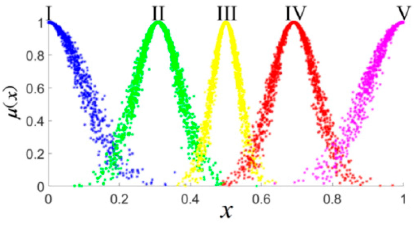
Cloud Model (CM)

The CM is a model for the conversion of qualitative concepts and quantitative values proposed on the basis of fuzzy set theory and probability, and it can reveal the inherent relevance of the randomness and ambiguity of certain factors or concepts themselves [27]. It was first proposed in 1995 by Li Deyi, an academician of the Chinese Academy of Engineering, and has been applied in many fields, such as risk assessment [28] and engineering benefit evaluation [29]. A CM can take the form of a rectangular cloud, trapezoidal cloud, normal cloud, etc. The normal CM is widely used due to its unique mathematical characteristics and versatility.

(1) Definition of Normal Cloud

Definition of normal cloud: Assume that U is a quantitative domain and expressed by precise numerical values, and C is a qualitative concept of U. A normal cloud can be defined if the quantitative value x$\in$U, and x is a random realization of the qualitative concept C, if it satisfies x~N(E_x, E_n²), where E_n²~N(E_n, H_e²), and the degree of membership to C satisfies:

$$\mu (x)=e^{[-\frac{{(x-E_x)}^2}{2{(E_n)}^2}]}$$

(1)

where E_x is the expected value; E_n is the entropy value; H_e is the super entropy.

(2) Digital Characteristics of CM

The CM includes the following three digital features: expected value E_x, entropy E_n, and super entropy H_e. Among them, E_x represents the expected value of the CM, which is a central value of the qualitative concept C in U, which is the most typical point with which to quantify the concept; E_n, as a metric, is determined by both randomness and ambiguity, and the larger its value is, the more qualitative the concept is, making it difficult to quantify its certainty; H_e is a metric that measures the uncertainty of entropy, which is related to the degree of dispersion of cloud droplets, and can indirectly reflect the thickness of the cloud. A schematic diagram of the digital features of a CM is shown in Figure 1.

(3) Cloud Generator

The cloud generator is used to convert qualitative indicators and quantitative values into one another. There are three types of cloud generators: (1) Forward Cloud Generator (FCG), which converts qualitative to quantitative—the calculation flowchart of the FCG is shown in Figure 2; (2) Backward Cloud Generator (BCG), which converts qualitative to qualitative; (3) X cloud generator and Y cloud generator constitute a special conditional cloud generator, in which C (E_x, E_n, H_e) is known and a specific value X or Y is used to calculate the degree of certainty.

The X condition cloud generator is used to calculate the cloud digital characteristics of each evaluation index, and the equations [30] are:

$$\begin{array}{l}E{x}_{ij}=\frac{x_{ij,1}+x_{ij,2}}{2}\\ E{n}_{ij}=\frac{x_{ij,1}-x_{ij,2}}{2.355}\end{array}$$

(2)

where $E_{x_{ij}},\hspace{0.17em}{E}_{n_{ij}}$ represent the expected value and entropy value, respectively, of the i-th index corresponding to the j-th serviceability grade; x_ij represents the membership value of the i-th index corresponding to the j-th serviceability grade; $x_{ij,1},\hspace{0.17em}{x}_{ij,2}$ represents the upper and lower boundary values, respectively, of the evaluation index system standard; the super entropy $H_{e_{ij}}$ is generally obtained by experience.

(4) Related calculations on CM

When the CM theory is used to transform qualitative concepts into quantitative values, the following steps will be taken: let the middle cloud be C₀ (E_x0, E_n0, H_e0), and the adjacent clouds on the left and right are C₋₁ (E_x−1, E_n−1, H_e−1), C₊₁ (E_x+1, E_n+1, H_e+1) and C₋₂ (E_x−2, E_n−2, H_e−2), C₊₂ (E_x+2, E_n+2, H_e+2). The cloud algorithms are as follows [31]:

$$\begin{array}{l}{E}_{x0}=\frac{(X_{\min }+X_{\max })}{2}\\ E_{x-2}=X_{\min }\\ E_{x+2}=X_{\max }\\ E_{x1}=E_{x0}-0.382\frac{(X_{\min }+X_{\max })}{2}\\ E_{x+1}=E_{x0}+0.382\frac{(X_{\min }+X_{\max })}{2}\end{array}$$

(3)

$$\begin{array}{l}{E}_{n-1}=E_{n+1}=0.382\frac{X_{\max }-X_{\min }}{6}\\ E_{n0}=0.618E_{n+1}\\ E_{n-2}=E_{n+2}=\frac{E_{n+1}}{0.618}\end{array}$$

(4)

$$\begin{array}{l}{H}_{e-1}=H_{e+1}=\frac{H_{e0}}{0.618}\\ H_{e-2}=H_{e+2}=\frac{H_{e+1}}{0.618}\end{array}$$

(5)

Among them, the super entropy H_e is the uncertainty of entropy, which is related to the discrete degree of cloud droplets and can indirectly reflect the thickness of clouds. The larger the H_e is, the more discrete the cloud droplets tend to be, which can be generally taken empirically; here, H_e is taken as 0.005 [32].

When solving the digital characteristics of the CM of the evaluation target, the influence of the weight values on the evaluation result is often comprehensively considered, and the following equation is used to solve the problem [33].

$$\left\{\begin{array}{c}{E}_x=\frac{E_{x1}{w}_1+E_{x2}{w}_2+\cdots +E_{xn}{w}_n}{w_1+w_2+\cdots +w_n}\\ E_n=\frac{w_1^2}{w_1^2+w_2^2+\dots w_n^2}{E}_{n1}+\frac{w_2^2}{w_1^2+w_2^2+\dots w_n^2}{E}_{n2}+\dots +\frac{w_n^2}{w_1^2+w_2^2+\dots w_n^2}{E}_{nn}\\ H_e=\frac{w_1^2}{w_1^2+w_2^2+\dots w_n^2}{H}_{e1}+\frac{w_2^2}{w_1^2+w_2^2+\dots w_n^2}{H}_{e2}+\dots +\frac{w_n^2}{w_1^2+w_2^2+\dots w_n^2}{H}_{en}\end{array}\right.$$

(6)

2.2. Weight Calculation Method

2.2.1. Analytic Hierarchy Process (AHP)

The AHP is a structural weight calculation method that was proposed by the American operations researcher TL Satty [34] in order to solve the problem of electricity distribution to various industrial sectors in the United States using system engineering theory and multi-objective and multi-attribute comprehensive evaluation criteria. The main steps of the method are as follows:

(1) Build a hierarchical structure model

The element at the top layer is called the target layer, which contains only one element and plays a role of overall dominance; the element at the bottom is the index layer, which is the basis of the entire evaluation system; the element between the top and the bottom is the middle layer, and the middle layer can be composed of multiple layers and should be analyzed according to specific problems.

(2) Construct a judgment matrix

Constructing judgment matrix is one of the core elements of AHP. In order to determine the relationship between different layers or elements of the same layer, it is necessary to establish a comparative judgment matrix and determine the affiliation relationship through matrix analysis. AHP is a more subjective means of determining the weight of factors by expert scoring, i.e., to compare two factors in order to obtain the relative importance of both. For the comparison criterion of elements a_ij, each factor is compared two by two, and the relationship between the i-th factor and the j-th factor is quantified to reflect the difference between them. The value range of a_ij is generally expressed by the 1–9 scale method (

Table 1. 1–9 proportional scale table.

Quantized Value	Level of Importance
1	Equivalent
3	Slightly important
5	More important
7	Very important
9	Extremely important
2, 4, 6, 8	Mid-point between two importance levels

) and the corresponding reciprocal.

(3) Weight assignment and consistency check

Step 1: Multiply each element by rows to obtain u_ij; see Equation (7). Step 2: Take u_ij to the power of n to obtain u_i; see Equation (8). Step 3: Normalize u_i to obtain the weight vector ${\mathsf{\omega }}_i$; see Equation (9). Step 4: Calculate the maximum characteristic root ${\lambda }_{\max }$ of the judgment matrix; see Equation (10).

$$u_{ij}={\displaystyle \prod _{j=1}^n{b}_{ij}}$$

(7)

$$u_i=\sqrt[n]{u_{ij}}$$

(8)

$${\mathsf{\omega }}_i=\frac{u_i}{{\displaystyle \sum _{i=1}^n{u}_i}}$$

(9)

$${\lambda }_{\max }={\displaystyle \sum _{i=1}^n\frac{{(A\mathsf{\omega })}_i}{n{\mathsf{\omega }}_i}}$$

(10)

where b_ij is the relatively important value of the i-th evaluation index relative to the j-th evaluation index, which is the value in the judgment matrix; A is the judgment matrix; $\mathsf{\omega }$ is the eigenvector; n is the number of elements.

After the weights are calculated, a consistency check is also needed. Only the calculated results that pass the consistency check have an acceptable degree of reliability. The consistency check usually uses the consistency ratio CR as the check standard, which is defined as $CR=\frac{CI}{RI}$, where CI is a consistency index, and its calculation equation is $CI=\frac{{\lambda }_{\max }-n}{n-1}$. RI is the average random consistency index, which is related to the order n of the judgment matrix, which can be found in

Table 2. Average random consistency index RI.

n	1	2	3	4	5	6	7	8	9
RI	0.00	0.00	0.58	0.9	1.12	1.24	1.32	1.41	1.45

.

Generally, when CR < 0.1, the consistency of the calculation result is considered acceptable; when CR ≥ 0.1, the consistency check fails, and the judgment matrix should be reconstructed for calculation until the calculation results are accepted when CR < 0.1.

(4) Hierarchical total ranking

The ranking of factors mainly involves a hierarchical ranking approach under a single criterion. In the case of the target layer, a total structural ranking of each factor is required to determine its level of importance.

2.2.2. Simple Correlation Function Method (SCF)

The SCF is based on the matter-element extension theory for related calculations. Extenics theory can mainly be divided into matter-element theory, extension set theory and extension logic. The matter-element theory solves the uncertainty and fuzziness, which is its main advantage [35]. SCF is a method that can be used to objectively determine the weight, and the calculation process [36] is as follows:

$$\begin{array}{cc}\mathrm{Assume}& \\ & r_{ij}(v_i,V_{ij})=\left\{\begin{array}{c}\frac{2(v_i-a_{ij})}{b_{ij}-a_{ij}},v_i\le \frac{a_{ij}+b_{ij}}{2}\\ \frac{2(b_{ij}-v_i)}{b_{ij}-a_{ij}},v_i\ge \frac{a_{ij}+b_{ij}}{2}\end{array}\right.\end{array}$$

(11)

$$V_{ij}=\left[\begin{array}{c}〈a_{1j},b_{1j}〉\\ 〈a_{2j},b_{2j}〉\\ ⋮\\ 〈a_{nj},b_{nj}〉\end{array}\right]$$

(12)

where r_ij represents the correlation of the i-th index and the j-th evaluation grade; v_i represents the sample value of the i-th index; V_ij represents the value range of the i-th index corresponding to the j-th evaluation grade, and its value is $V_{ij}=〈a_{ij},b_{ij}〉$; $a_{ij}$ is the lower limit of the value of the i-th index, and b_ij is the upper limit of the value of the i-th index. Moreover, i = 1, 2, ⋯, n; j = 1, 2, ⋯, m.

$$V_{iP}=\left[\begin{array}{c}〈a_{1P},b_{1P}〉\\ 〈a_{2P},b_{2P}〉\\ ⋮\\ 〈a_{nP},b_{nP}〉\end{array}\right]$$

(13)

If $v_i\in V_{iP},(i=1,2,\cdots ,n)$, where V_iP is the range measured by the object to be evaluated, and its value is $V_{iP}=〈a_{iP},b_{iP}〉$, a_iP is the minimum value of the lower boundary of the i-th index in all evaluations, b_iP is the maximum value of the upper boundary of the i-th feature in all evaluations, and $V_{ij}\subset V_{iP} (i=1,2,\cdots ,n; j=1,2,\cdots ,m)$. Then $r_{i{j}_{\max }}(v_i,V_{ij})=\underset{j\in (1,2,\cdots ,\hspace{0.17em}m)}{\max }\left\{r_{ij}(v_i,V_{ij})\right\}$.

If the evaluation grade j of the evaluation index i of the object to be evaluated is larger, and the weight assigned by the index is greater, then take:

$$r_i=\{\begin{array}{c}{j}_{\max }\times (1+r_{i{j}_{\max }}(v_i,V_{ij})), r_{i{j}_{\max }}(v_i,V_{ij})\ge -0.5\\ j_{\max }\times 0.5, r_{i{j}_{\max }}(v_i,V_{ij})<-0.5\end{array}$$

(14)

Among them, j_max represents the evaluation grade into which the sample value of index i in the element to be evaluated falls, and the larger the value, the more restrictive the index is to treat the matter, when $r_{i{j}_{\max }}=r_{im}$, $j_{\max }=\max \left\{m\right\}$.

If the evaluation grade j of the evaluation index i of the object to be evaluated is larger, the weight assigned by the index is smaller, taking:

$$r_i=\{\begin{array}{c}(m-j_{\max }+1)\times (1+r_{i{j}_{\max }}(v_i,V_{ij})), r_{i{j}_{\max }}(v_i,V_{ij})\ge -0.5\\ (m-j_{\max }+1)\times 0.5, r_{i{j}_{\max }}(v_i,V_{ij})<-0.5\end{array}$$

(15)

Among them, m—represents the number of categories divided for each index, when $r_{i{j}_{\max }}=r_{im}$, $j_{\max }=\min \left\{m\right\}$.

Then, the weight of the index is

$$w_i=\frac{r_i}{{\displaystyle \sum _{i=1}^n{r}_i}}$$

(16)

Among them, w_i is the normalized value of the i-th evaluation index weight.

2.2.3. Game Theory Combination Weighting Method

The subjective weighting method, used to determine the weight of each indicator, is mainly based on the experience and subjective preferences of decision-makers in the relevant field of knowledge, and these methods either have a large subjective factor or do not consider the importance of the indicators themselves to the problem. However, in practical evaluation problems, the importance of indicator factors is not affected by the subjective factors of decision-makers and is objective, and only the combination of subjective and objective weights can reflect the importance of evaluation indicators. In the game theory combination weighting method, the participants in the game are the objective weight coefficient and subjective weight coefficient of each evaluation index; the equilibrium condition of the game is that the deviation between the weight of each evaluation index and the basic weight is the smallest.

The specific calculation steps [37] are as follows:

(i) Use m different weighting methods to weight the evaluation indicators, and construct the basic weight vector set of the evaluation indicators as $w_k=\left\{w_{k1},w_{k2},\cdots ,w_{kn}\right\}(k=1,2,\cdots ,m)$; then, the m linear combinations are:

$$w={\displaystyle \sum _{k=1}^m{\alpha }_k}{w}_k^T({\alpha }_k>0,{\displaystyle \sum _{k=1}^m{\alpha }_k}=1)$$

(17)

In the equation, w is a possible weight vector of the evaluation index weight set; ${\alpha }_k$ is the linear combination coefficient.

(ii) Minimize the deviation between w and each w_k, namely:

$$\min {‖{\displaystyle \sum _{j=1}^m{\alpha }_j}{w}_j^T-w_i‖}_2\hspace{1em}(i,j=1,2,\cdots ,n)$$

(18)

(iii) Solve the linear combination coefficient. From the properties of matrix differentiation, it can be seen that the optimal first-order derivative condition equivalent to Equation (18) is:

$${\displaystyle \sum _{j=1}^m{\alpha }_j}{w}_i{w}_j^T=w_i{w}_i^T$$

(19)

Equation (19) corresponds to the following linear equations:

$$\left[\begin{array}{cccc}{w}_1·w_1^T& w_1·w_2^T& \cdots & w_1·w_n^T\\ w_2·w_1^T& w_2·w_2^T& \cdots & w_2·w_n^T\\ \cdots & \cdots & \cdots & \cdots \\ w_n·w_1^T& w_n·w_2^T& \cdots & w_n·w_n^T\end{array}\right]·\left[\begin{array}{c}{\alpha }_1\\ {\alpha }_2\\ \cdots \\ {\alpha }_n\end{array}\right]=\left[\begin{array}{c}{w}_1·w_1^T\\ w_2·w_2^T\\ \cdots \\ w_n·w_n^T\end{array}\right]$$

(20)

(iv) The weight coefficient is normalized. According to the calculation, $({\alpha }_1,{\alpha }_2,\cdots ,{\alpha }_n)$ can be obtained, and then the weight coefficient can be normalized to obtain:

$${\alpha }_k^{\ast }=\frac{{\alpha }_k}{{\displaystyle \sum _{k=1}^m{\alpha }_k}} (k=1,2,\cdots ,m)$$

(21)

(v) Solve the final combination weight. Based on game theory, the combined weight of the evaluation index is obtained as:

$$w^{\ast }={\displaystyle \sum _{k=1}^m{\alpha }_k^{\ast }}{w}_k^T$$

(22)

3. Case Study

3.1. Engineering Case

In order to verify the science and rationality of the method proposed in this paper, a canal in Henan Province was used as an example to carry out the applied research. The canal is located in the Eastern Henan plain on the south bank of the Yellow River and belongs to the Zhaokou Yellow River diversion irrigation area project. The project was built in 1970 and irrigation was started in the following year. The designated irrigation area is 967,653.2 acres (339,595.4 ha). The canal passes through 14 counties (districts) in five places, namely Zhengzhou City, Kaifeng City, Xuchang City, Zhoukou City, and Shangqiu City. It has been 51 years since the first phase of the project. A field inspection confirmed that the CL slabs along the route had been damaged, and the occurrence of damage due to frost heave, cracking of the concrete lining, canal landslides, lining bulging, lining uplift, lining instability and slumping, canal panel dislocation and other faults were observed. A method for the evaluation of the serviceability status of the CL in the first phase of the project is very important for the repair and maintenance of the CL. The geographic location and damage distribution status are shown in Figure 3.

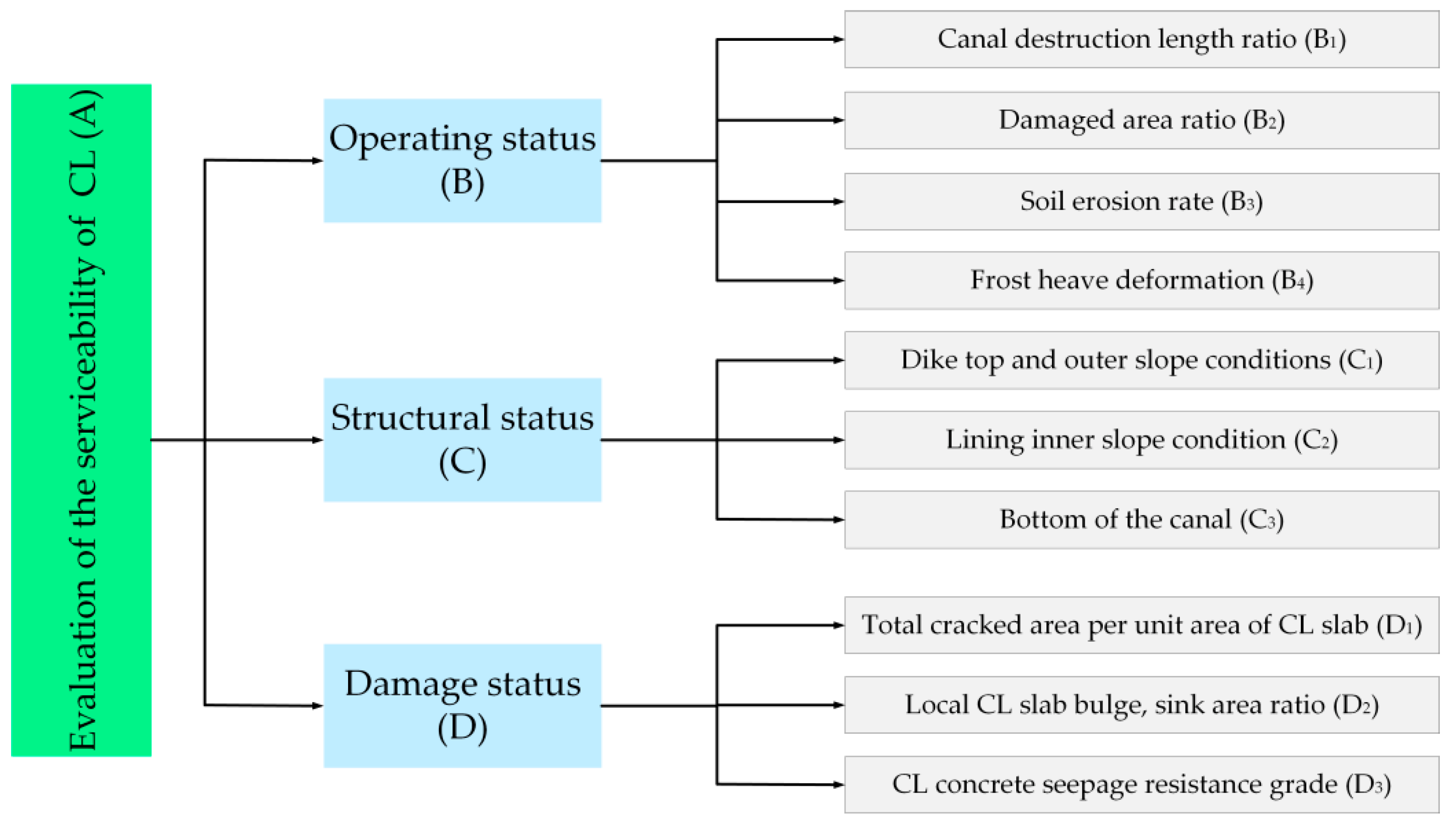
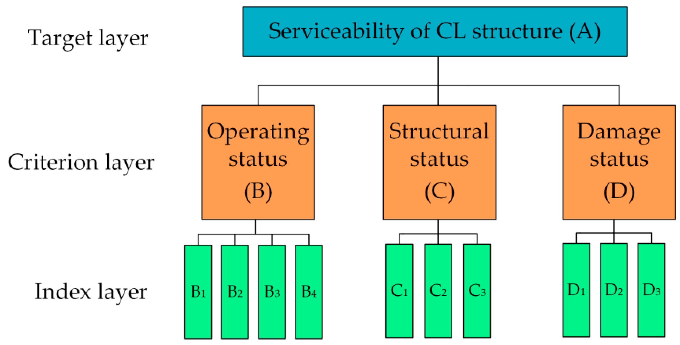
3.2. Selection of Evaluation Indicators of the Serviceability of CL Structure

Through on-site investigation, a literature search, expert consultation and so on, combined with the “Technical Specification for Irrigation Canal Lining Engineering” (DB 64/T 811—2012) [38], the factors affecting the serviceability of the CL structure were divided into three major factors: operating status, structural status and damage status. Each factor was composed of several evaluation indicators. The specific classification is shown in Figure 4.

3.3. Determining the Evaluation Grade of the Serviceability of a CL Structure

The “Technical Specification for Irrigation Canal Lining Engineering” (DB 64/T 811—2012) [38] divides the serviceability of the CL engineering into 5 grades, which are good, basically good, minor damage, major damage and severe damage. This paper refers to the specification and similarly divides the serviceability of the CL into five grades, as shown in

Table 3. Serviceability classification of CL structure.

Evaluation Grade	Serviceability of CL Structure
I	Good
II	Basically good
III	Minor damage, needs minor repair
IV	Major damage, needs major repair
V	Severe damage, cannot be used

.

Table 3 contains qualitative descriptions; in actual engineering, some CL serviceability evaluation indices are characterized by fuzziness when they are divided, and it is difficult to accurately classify which grade they belong to, while CM theory can simultaneously reflect the randomness and fuzziness of describing such factors, transform the uncertainty relationship between qualitative and quantitative entities and form a mapping relationship between qualitative and quantitative, which can be used to address the uncertainty of fuzziness factors [39]. Therefore, the CM theory method is used to devise the serviceability evaluation indicators for the CL structure with the normal CM, and Equations (3)–(5) are used to transform the qualitative concepts of the five grades in Table 3 into five cloud models, where the domain is [0, 1], and the results are shown in

Table 4. Serviceability evaluation grade CM of CL structure.

Evaluation Grade	Qualitative Description	Cloud Model (Ex, En, He)
I	Good	(0.000, 0.104, 0.013)
II	Basically good	(0.309, 0.064, 0.008)
III	Minor damage, needs minor repair	(0.500, 0.039, 0.005)
IV	Major damage, needs major repair	(0.691, 0.064, 0.008)
V	Severe damage, cannot be used	(1.000, 0.104, 0.013)

.

FCG is used to generate a cloud image from the evaluation grade CM, in which the number of cloud drops is 1500, and the cloud image is drawn with the help of MATLAB software; the result is shown in Figure 5.

3.4. Determining the Evaluation Standard of the Serviceability of a CL Structure

The specific numerical interval of each grade refers to the “Technical Specification for Irrigation Canal Lining Engineering” (DB 64/T 811—2012) [38], “Standard for Quality Control of Concrete” (GB 50164-2011) [40] and “Standard for test methods long-term performance and durability of ordinary concrete” (GB/T50082-2009) [41]. The evaluation criteria for a CL with a pile number of DYG0+000 to DYG3+331.5 were divided, as shown in

Table 5. Evaluation criteria for the serviceability of a CL structure.

Serial Number (SN)	I	II	III	IV	V
B1	(0, 5%)	[5%, 10%)	[10%, 20%)	[20%, 30%)	[30%, 50%)
B2	(0, 5%)	[5%, 10%)	[10%, 20%)	[20%, 30%)	[30%, 40%)
B3	(0, 5%)	[5%, 10%)	[10%, 20%)	[20%, 30%)	[30%, 60%)
B4	(0, 10]	(10, 20]	(20, 30]	(30, 40]	(40, 50]
C1	The road surface of canal is flat, and the outer slope is smooth	The road surface of canal is flat on average, and the outer slope is smooth	The road surface on the top of canal has small pits, and the outer slope is locally convex	The road surface of canal has large pits, and the outer slope is partially collapsed	There are many pits on the road surface on the top of the canal, and there are many local collapses on the outer slope
C2	Slope: smooth. The concrete slab is filled with joints to keep it intact	Slope: smooth. The concrete slab filling is basically intact	Slope: smooth. There are cracks in the partial slab	The slope surface is flat, and there are many cracks in the local slab.	Slope concrete slab is loose. Many cracks in the soil slab
C3	The canal bottom is flat, and the concrete lining at the canal bottom has no deformation.	The canal bottom is flat, and there are slight cracks in the bottom of concrete slab.	The canal bottom is basically kept flat, and the canal bottom surface has slight peeling.	The canal bottom is eroded, and the lining concrete has collapsed.	The scouring depth at the bottom of the canal is large, and the lining concrete has collapsed and bulges seriously.
D1	(0, 100]	(100, 400]	(400, 700]	(700, 1000]	(1000, 1500]
D2	(0, 5%)	[5%, 10%)	[10%, 20%)	[20%, 30%)	[30%, 45%)
D3	[14, 12]	(12, 10]	(10, 8]	(8, 6]	(6, 4]

Note: For B₁, B₂, B₃, B₄, C₁, C₂, C₃, D₂ each evaluation grade or qualitative description is based on the “Technical Specification for Irrigation Canal Lining Engineering” (DB 64/T 811—2012) [38]. D₁: The division of the evaluation grade of the total cracked area per unit area of the CL slab is based on the specification “Standard for Quality Control of Concrete” (GB 50164-2011) [40]. D₃: The CL concrete seepage resistance grade is determined by taking the CL concrete after standard curing for 28 d age as the standard specimen, and the maximum water pressure that can be withstood during the seepage resistance performance test according to the “Standard for test methods long-term performance and durability of ordinary concrete” (GB/T50082-2009) [41]. The grade classification is based on the “Standard for Quality Control of Concrete” (GB 50164-2011) [40]. For each evaluation index, if the actual quantified value exceeds or falls below the upper and lower limit values of the interval corresponding to the evaluation grade I or V in Table 5, the value can be the upper or lower limit value of the interval corresponding to the evaluation grade I or V.

.

3.5. Quantitative and Qualitative Evaluation Indicators

In actual engineering, some evaluation indicators are difficult to quantify, and often rely on qualitative evaluation in order to describe the object to be evaluated. For these non-quantitative evaluation indicators, the indicators are often quantified through the expert scoring method. Referring to the division method in the literature [42], for the condition of the dike top and outer slope, it is stipulated that: (100~90) means that the condition is good, the dike top pavement is relatively flat, the outer slope is flat and so on; (89~80) indicates basically good condition, the dike top pavement is flat in general, and the outer slope is flat; (79~70) indicates that the engineering condition includes minor damage, the dike top pavement has small local pits and depressions; (69~60) indicates that the engineering condition includes major damage, the top pavement has large pits and undulations; (59~50) indicates that the engineering condition includes serious damage, the top pavement has many pits and undulations, and the outer slope is partially collapsed. Similarly, according to Table 5, the values of the inner slope lining condition and canal bottom condition quantified in turn are not listed here, and the final results are shown in

Table 6. Quantitative evaluation criteria for the serviceability of a CL structure.

SN	I	II	III	IV	V
B1	(0, 5%]	(5%, 10%]	(10%, 20%]	(20%, 30%]	(30%, 50%]
B2	(0, 5%]	(5%, 10%]	(10%, 20%]	(20%, 30%]	(30%, 40%]
B3	(0, 5%]	(5%, 10%]	(10%, 20%]	(20%, 30%]	(30%, 60%]
B4	(0, 10]	(10, 20]	(20, 30]	(30,40]	(40, 50]
C1	[100, 90)	[90, 80)	[80, 70)	[70, 60)	[60, 50)
C2	[100, 90)	[90, 80)	[80, 70)	[70, 60)	[60, 50)
C3	[100, 90)	[90, 80)	[80, 70)	[70, 60)	[60, 50)
D1	(0, 100]	(100, 400]	(400, 700]	(700, 1000]	(1000, 1500]
D2	(0, 5%)	[5%, 10%)	[10%, 20%)	[20%, 30%)	[30%, 45%)
D3	[14, 12]	(12, 10]	(10, 8]	(8, 6]	(6, 4]

.

3.6. Determining the Evaluation Index Weight of the Serviceability of a CL Structure

When calculating the weight, it is necessary to determine the relationship between the measured sample data and the standard data of each evaluation index in each serviceability evaluation grade, and to compare the standard value of each evaluation index with the measured sample value. Here, the extension matter-element theory is used to establish the relationship between the standard value of each evaluation indicator level and the measured sample data for each serviceability evaluation index.

In order to ensure the comparability of the different evaluation indicators, the range change method is used to normalize and non-dimensionalize the indicator data. For indicators numbered B₁, B₂, B₃, B₄, D₁, D₂, the influence of these factors on the serviceability of the lining structure is positively correlated. The larger the value, the worse the serviceability, which is handled as follows: $X_i=\frac{X_i-X_{i\min }}{X_{i\max }-X_{i\min }}$. For index numbers C₁, C₂, C₃, D₃, these factors are negatively related to the serviceability of the lining structure. The smaller the value, the worse the serviceability, which is handled as follows: $X_i=\frac{X_{i\max }-X_i}{X_{i\max }-X_{i\min }}$. The range of each index grade after treatment is shown in

Table 7. Standard data for evaluation index of lining serviceability after normalization.

SN	I	II	III	IV	V
B1	(0, 0.10]	(0.10, 0.20]	(0.20, 0.40]	(0.40, 0.6]	(0.60, 1]
B2	(0, 0.13]	(0.13, 0.25]	(0.25, 0.50]	(0.5, 0.75]	(0.75, 1]
B3	(0, 0.08]	(0.08, 0.17]	(0.17, 0.33]	(0.33, 0.5]	(0.50, 1]
B4	(0,0.20]	(0.20, 0.40]	(0.40, 0.60]	(0.60, 0.80]	(0.80, 1]
C1	[0, 0.20)	[0.20, 0.40]	(0.40, 0.60]	(0.60, 0.80]	(0.80, 1]
C2	[0, 0.20)	[0.20, 0.40]	(0.40, 0.60]	(0.60, 0.80]	(0.80, 1]
C3	[0, 0.20)	[0.20, 0.40]	(0.40, 0.60]	(0.60, 0.80]	(0.80, 1]
D1	(0, 0.07]	(0.07, 0.27]	(0.27, 0.47]	(0.47, 0.67]	(0.67, 1]
D2	(0, 0.11]	(0.11, 0.22]	(0.22, 0.44]	(0.44, 0.67]	(0.67, 1]
D3	[0, 0.20)	[0.20, 0.40]	(0.40, 0.60]	(0.60, 0.80]	(0.80, 1]

.

The inspection data of B₁ are based on the ratio of the measured value of the actual damage length of the canal to the total length of the canal, and the cumulative damage length measured on site is 1399.25 m, accounting for 0.42 of the total length (3331.5 m); the inspection data of B₂ are based on the ratio of the measured value of the actual damage area of the canal to the total area of the effective water delivery area of the canal, and the total area of the slope and bottom of the canal on both sides is 37,312.8 square meters, and the cumulative calculation of the damaged area is 13,059.62 square meters, accounting for 0.35 of the total area; the inspection data of B₃ are obtained by taking soil sample from the site, then carry out the washout test [43] on the soil sample, finally the result of the soil erosion rate is 0.51; the inspection data of B₄ are based on the ratio of the measured value of the actual frost heave deformation thickness in some areas of the canal to the normal thickness of the canal; the inspection data of C₁, C₂ and C₃ are all based on the actual CL conditions and the experts’ scores, for which the geometric average is calculated; the inspection data of D₁ are the ratio of the cracked area per unit area of the CL slab to the total area of the slab, which is calculated by geometrically averaging the ratio of all the damaged slabs, and we measured the average cracked area per square meter of a single plate as 1200 mm²; the inspection data of D₂ are the ratio of the local uplift and subsidence area of the CL board to the total area, and the difference between B₂ is that only refers to a number of local plates occurring uplift and subsidence damage, and then the area of damage to the ratio of the area of the plate is the result, after field testing and data statistics, it is found that the average value is 40%; the inspection data of D₃ is to make the test piece according to the mix ratio of the lining concrete of the canal, and then put it into the standard curing room after curing for 28 days, then the gradual pressure method is used to carry out the concrete impermeability test, and the water pressure is applied step by step to determine the concrete seepage resistance grade. When water seepage occurs on the specimen surface, record the water pressure that causes the specimen to seep. Through impermeability test of the CL concrete specimens, the result of the concrete seepage resistance grade is 8. The following formula [40] is used to calculate the grade of concrete seepage resistance:

$$P=10H-1$$

(23)

where, P is the concrete seepage resistance grade; H is the water pressure (MPa) when the test piece is seeping.

The SCF is used to determine the index weight, and the data in

Table 8. Normalized value of test data of each evaluation index of a certain canal.

SN	I	II	III	IV	V	Inspection Data	Normalized
B1	(0, 0.10]	(0.10, 0.20]	(0.20, 0.40]	(0.40, 0.6]	(0.60, 1]	42%	0.840
B2	(0, 0.13]	(0.13, 0.25]	(0.25, 0.50]	(0.5, 0.75]	(0.75, 1]	35%	0.875
B3	(0, 0.08]	(0.08, 0.17]	(0.17, 0.33]	(0.33, 0.5]	(0.50, 1]	51%	0.850
B4	(0, 0.20]	(0.20, 0.40]	(0.40, 0.60]	(0.60, 0.80]	(0.80, 1]	39	0.780
C1	[0, 0.20)	[0.20, 0.40]	(0.40, 0.60]	(0.60, 0.80]	(0.80, 1]	56	0.880
C2	[0, 0.20)	[0.20, 0.40]	(0.40, 0.60]	(0.60, 0.80]	(0.80, 1]	67	0.660
C3	[0, 0.20)	[0.20, 0.40]	(0.40, 0.60]	(0.60, 0.80]	(0.80, 1]	59	0.820
D1	(0, 0.07]	(0.07, 0.27]	(0.27, 0.47]	(0.47, 0.67]	(0.67, 1]	1200	0.800
D2	(0, 0.11]	(0.11, 0.22]	(0.22, 0.44]	(0.44, 0.67]	(0.67, 1]	40%	0.889
D2	(0, 0.20)	[0.20, 0.40]	(0.40, 0.60]	(0.60, 0.80]	(0.80, 1]	8	0.600

are substituted into Equations (11)–(16) to obtain the weight of each evaluation index, as shown in

Table 9. Weights of evaluation indicators.

SN	B1	B2	B3	B4	C1	C2	C3	D1	D2	D3
Weight	0.122	0.136	0.109	0.065	0.122	0.087	0.082	0.122	0.114	0.041

.

The AHP method was used, and a total of 15 experts were invited from construction units, scientific research institutes, and supervision units to provide scores for the evaluation indicators, and the subsequent assignment is based on the results of the experts’ scoring. According to the actual situation of the project, the hierarchical structure model is constructed as shown in Figure 6.

The constructed criterion layer’s judgment matrix relative to the target layer is shown in

Table 10. Judgment matrix of criterion layer relative to target layer.

A	B	C	D	Weight
B	1	1/5	1/7	0.072
C	5	1	1/3	0.279
D	7	3	1	0.649
${\lambda }_{\max }$ = 3.065, CI = 0.032, RI = 0.58, CR = 0.056 < 0.10, consistency check passed

, and the index layer’s judgment matrix relative to the criterion layer is shown in

Table 11. Judgment matrix of index layer relative to criterion layer (B–B_1–4).

B	B1	B2	B3	B4	Weight
B1	1	3	5	3	0.490
B2	1/3	1	7	3	0.308
B3	1/5	1/7	1	1/3	0.059
B4	1/3	1/3	3	1	0.144
${\lambda }_{\max }$ = 4.235, CI = 0.078, RI = 0.9, CR = 0.087 < 0.10, consistency check passed

,

Table 12. Judgment matrix of index layer relative to criterion layer (C–C_1–3).

C	C1	C2	C3	Weight
C1	1	1/3	3	0.258
C2	3	1	5	0.637
C3	1/3	1/5	1	0.105
${\lambda }_{\max }$ = 3.039, CI = 0.019, RI = 0.58, CR = 0.033 < 0.10, consistency check passed

and

Table 13. Judgment matrix of index layer relative to criterion layer (D–D_1–3).

D	D1	D2	D3	Weight
D1	1	3	1/5	0.188
D2	1/3	1	1/7	0.081
D3	5	7	1	0.731
${\lambda }_{\max }$ = 3.065, CI = 0.032, RI = 0.58, CR = 0.056 < 0.10, consistency check passed

. Each judgment matrix has been checked for consistency.

The calculation results of the final weights are shown in

Table 14. Calculation results of subjective weight.

Index Layer	Single Weight			Weight Value
	B	C	D
	0.072	0.279	0.649
B1	0.490			0.0353
B2	0.308			0.0221
B3	0.059			0.0043
B4	0.144			0.0103
C1		0.258		0.0721
C2		0.637		0.1777
C3		0.105		0.0292
D1			0.188	0.1223
D2			0.081	0.0525
D3			0.731	0.4742

.

Obviously, the weights obtained by the AHP method and the SCF method show greater differences in the results of the same evaluation index, such as B₂, B₃, C₂ and D₃. The game theory combination weighting method can fully take into account the characteristics of each of the subjective and objective weighting methods in order to determine the level of agreement or compromise between the subjective and objective weight values, so that the deviation of the subjective and objective weights is minimized. In this study, there are two different assignment methods, so m = 2, and according to Equations (17)–(22), the integrated weight coefficient vector ${\alpha }_1$ and ${\alpha }_2$ can be determined. The ${\alpha }_1$ = 0.707 and ${\alpha }_2$ = 0.293, and the final weight calculation results are shown in

Table 15. Final weight calculation results.

SN	Weights Determined Based on AHP	Weights Determined Based on the SCF	Weights Determined Based on Game Theory
B1	0.0353	0.122	0.061
B2	0.0221	0.136	0.055
B3	0.0043	0.109	0.035
B4	0.0103	0.065	0.026
C1	0.0721	0.122	0.087
C2	0.1777	0.087	0.151
C3	0.0292	0.082	0.045
D1	0.1223	0.122	0.122
D2	0.0525	0.114	0.071
D3	0.4742	0.041	0.347

.

3.7. Determining the Overall Serviceability of a CL Structure

Equation (2) is used to obtain the standard CM of each evaluation index, as shown in

Table 16. Standard CM of various evaluation indicators for a CL.

SN	I	II	III	IV	V
B1	(0.050, 0.042, 0.005)	(0.150, 0.042, 0.005)	(0.300, 0.085, 0.005)	(0.500, 0.085, 0.005)	(0.800, 0.170, 0.005)
B2	(0.065, 0.055, 0.005)	(0.190, 0.051, 0.005)	(0.375, 0.106, 0.005)	(0.625, 0.106, 0.005)	(0.875, 0.106, 0.005)
B3	(0.040, 0.034, 0.005)	(0.125, 0.038, 0.005)	(0.250, 0.068, 0.005)	(0.415, 0.072, 0.005)	(0.750, 0.212, 0.005)
B4	(0.100, 0.085, 0.005)	(0.300, 0.085, 0.005)	(0.500, 0.085, 0.005)	(0.700, 0.085, 0.005)	(0.900, 0.085, 0.005)
C1	(0.100, 0.085, 0.005)	(0.300, 0.085, 0.005)	(0.500, 0.085, 0.005)	(0.700, 0.085, 0.005)	(0.900, 0.085, 0.005)
C2	(0.100, 0.085, 0.005)	(0.300, 0.085, 0.005)	(0.500, 0.085, 0.005)	(0.700, 0.085, 0.005)	(0.900, 0.085, 0.005)
C3	(0.100, 0.085, 0.005)	(0.300, 0.085, 0.005)	(0.500, 0.085, 0.005)	(0.700, 0.085, 0.005)	(0.900, 0.085, 0.005)
D1	(0.035, 0.085, 0.005)	(0.170, 0.085, 0.005)	(0.370, 0.085, 0.005)	(0.570, 0.085,0.005)	(0.835, 0.140, 0.005)
D2	(0.055, 0.047, 0.005)	(0.165, 0.047, 0.005)	(0.330, 0.093, 0.005)	(0.555, 0.098, 0.005)	(0.835, 0.140, 0.005)
D3	(0.100, 0.085, 0.005)	(0.300, 0.085, 0.005)	(0.500, 0.085, 0.005)	(0.700, 0.085, 0.005)	(0.900, 0.085, 0.005)

. The CM theory is used to calculate the related inspection data of the CL in order to obtain the measured CM of each index, as shown in

Table 17. CM of each test index of a CL.

SN	Cloud Model (Ex, En, Ee)
B1	(0.920, 0.068, 0.005)
B2	(0.938, 0.053, 0.005)
B3	(0.925, 0.064, 0.005)
B4	(0.790, 0.008, 0.005)
C1	(0.940, 0.051, 0.005)
C2	(0.730, 0.059, 0.005)
C3	(0.910, 0.076, 0.005)
D1	(0.900, 0.085, 0.005)
D2	(0.945, 0.047, 0.005)
D3	(0.600, 0.085, 0.005)

.

According to the established CL structure serviceability evaluation index system, the index CM and index weights are calculated and solved gradually from the index layer to the target layer until the target layer CM is solved, i.e., the comprehensive evaluation result CM is obtained. Equation (6) was used for the calculation, and the results are shown in

Table 18. CM data for evaluation results of indicators at all layers.

Target Layer	Final Cloud Model	Criterion Layer	Indicator Cloud Model
A	(0.799, 0.077, 0.005)	B	(0.907, 0.057, 0.005)
		C	(0.823, 0.058, 0.005)
		D	(0.713, 0.084, 0.005)

.

From the comprehensive evaluation results of the CM in Figure 7, it can be seen that the serviceability of the CL is between IV and V and is biased toward IV. According to the principle of maximum affiliation, it is selected as IV, which means that the canal as a whole is graded as having major damage, which is consistent with the actual situation of the first phase of the Yellow River diversion irrigation district project, indicating the accuracy and rationality of the method. By comparison with Figure 8, it is found that the evaluation results of the criterion layers are B = V, C = IV (according to the numerical characteristics of the CM of criteria layer C in Table 18, the expected value is 0.823, while comparing the values of the cloud models of grade IV and V, the middle value of the two expected values is 0.845, and C is closer to grade IV, which is determined as level IV according to the principle of maximum subordination) and D = IV, respectively. The results show that the CL is seriously damaged.

The final evaluation result CM is:

Figure 7. Comprehensive evaluation result of CM of the CL serviceability.

Figure 7. Comprehensive evaluation result of CM of the CL serviceability.

The CM of each evaluation index is:

Figure 8. Evaluation result of CM of the criterion layer index of the serviceability of a CL structure: (a) CM evaluation of operating status; (b) CM evaluation of structural status; (c) CM evaluation of damage status.

Figure 8. Evaluation result of CM of the criterion layer index of the serviceability of a CL structure: (a) CM evaluation of operating status; (b) CM evaluation of structural status; (c) CM evaluation of damage status.

3.8. Comparison with AHP–EW–UMT Evaluation Method

In order to further verify the science and rationality of the method proposed in this paper, a comparative study was conducted using AHP–EW–UMT. Entropy is an objective assignment method, which needs to be combined with other methods when evaluating an objective. UMT was first proposed by Chinese scholar Wang Guangyuan in 1990, and it is a new uncertainty information theory that can effectively quantify various uncertainty factors in order to perform evaluation. It has been widely used in the fields such as construction safety risk assessment [44]. In addition, the serviceability grade classification of the comparative study is divided into five grades as before.

The related concepts of UMT can be found in the literature [44] and are thus omitted here. The main calculation steps are as follows:

① Construct a single index measurement evaluation matrix

If ${\mu }_{ijk}=\mu (x_{ij}\in C_k)$ represents the degree to which the measured value x_ij belongs to the k-th evaluation grade C_k, and the requirements are satisfied:

$$0\le \mu (x_{ij}\in C_k)\le 1 (i=1,2,\cdots ,s;j=1,2,\cdots ,n;k=1,2\cdots ,m)$$

(24)

$$\mu (x_{ij}\in U)=1$$

(25)

$$\mu (x_{ij}\in \underset{l=1}{\overset{k}{\cup }}{C}_l)={\displaystyle \sum _{l=1}^k\mu (x_{ij}}\in C_l) (k=1,2,\cdots ,p)$$

(26)

Satisfaction of Equations (24)–(26) is referred to as the uncertainty measure, Considering matrix ${({\mu }_{ijk})}_{m\times p}$ a single–index unascertained measure evaluation matrix, we have:

$${({\mu }_{ijk})}_{m\times p}=\left[\begin{array}{cccc}{\mu }_{i11}& {\mu }_{i12}& \cdots & {\mu }_{i1p}\\ {\mu }_{i21}& {\mu }_{i22}& \cdots & {\mu }_{i2p}\\ ⋮& ⋮& \ddots & ⋮\\ {\mu }_{im1}& {\mu }_{im2}& \cdots & {\mu }_{imp}\end{array}\right]$$

(27)

Before establishing the single-index unascertained measure matrix, it is necessary to establish a single-index unascertained measure function (UMF). At present, the construction methods for single–index UMF mainly include linear, exponential, parabola, etc. Among them, the linear construction method has the characteristics of simple calculation and wide applicability, so the linear construction method is selected as the measurement function; the corresponding function graph is shown in Figure 9.

The UMF expression corresponding to Figure 9 is as follows:

$$\left\{\begin{array}{c}{\mu }_i(x)=\left\{\begin{array}{cc}\frac{-x}{a_{i+1}-a_i}+\frac{a_{i+1}}{a_{i+1}-a_i}& a_i<x<a_{i+1}\\ \hspace{1em}0\hfill & \hspace{0.17em}\hspace{0.17em}\hspace{0.17em}x>a_{i+1}\hfill \end{array}\right.\\ {\mu }_{i+1}(x)=\left\{\begin{array}{cc}\hspace{1em}0\hfill & \hspace{0.17em}\hspace{0.17em}x<a_i\hfill \\ \frac{x}{a_{i+1}-a_i}-\frac{a_i}{a_{i+1}-a_i}\hfill & a_i<x<a_{i+1}\end{array}\right.\end{array}\right.$$

(28)

where $a_i$, $a_{i+1}$ represent the value range of the index grade.

② Determine the index weight

Let w_j denote the relative importance of the measurement index X_j compared with other indices. It is required that w_j satisfies $0\le w_j\le 1$, and ${\displaystyle \sum _{j=1}^n{w}_j=1}$. w_j is called the weight of X_j, and $w=\left\{w_1,w_2,\cdots ,w_n\right\}$ is called the index weight vector set. The entropy weight theory can be used to determine the weight of the index, where $H_j(j=1,2,\cdots ,n)$ is the information entropy determined by the unascertained measure vector ${\mu }_{ijk}$, namely:

$$H_j=-{\displaystyle \sum _{k=1}^m{\mu }_{ijk}}\lg {\mu }_{ijk}$$

(29)

Let $v_j$ be the amount of information provided by the information entropy of the $j$-th evaluation index:

$$v_j=1-H_j=1+\frac{1}{\lg m}{\displaystyle \sum _{k=1}^m{\mu }_{ijk}}\lg {\mu }_{ijk}$$

(30)

The weight is:

$$w_j=\frac{v_j}{{\displaystyle \sum _{j=1}^n{v}_j}}$$

(31)

Given that the single index measurement evaluation matrix Equation (27) is known, w_j can be obtained by Equations (29)–(31).

③ Determine the evaluation vector of multi-index comprehensive measurement

Let ${\mu }_{ik}=\mu (P_i\in C_k)$ be the degree to which the evaluation sample P_i belongs to the k-th evaluation category C_k, then

$${\mu }_{ik}={\displaystyle \sum _{j=1}^n{w}_j}{\mu }_{ijk}(i=1,2,\cdots ,s;k=1,2,\cdots ,m)$$

(32)

Obviously $0\le {\mu }_{ik}\le 1$ and ${\displaystyle \sum _{k=1}^m{\mu }_{ik}}=1$, and Equation (32) as shown is an unascertained measure, so $\left\{{\mu }_{i1},{\mu }_{i2},\cdots ,{\mu }_{im}\right\}$ is called the multi-index comprehensive evaluation vector of P_i.

④ Credible degree recognition

In order to obtain the final evaluation result of the evaluation object, we introduce the credible degree recognition criteria: let $\lambda$($\lambda \ge 0.5$) be the credible degree, if $C_1>C_2>\cdots >C_m$, and let:

$$k_0=\min \left\{k:{\displaystyle \sum _{k=1}^m{\mu }_{ik}\ge \lambda (i=1,2,\cdots ,s)}\right\}$$

(33)

It is considered that the evaluation sample P_i belongs to the k₀ evaluation grade C_k0.

In this case, the specific calculation process is:

(1) Construct a single index measurement function

According to the definition of the single–indicator measurement function and the data in Table 8, the unconfirmed measurement function (UMF) of each evaluation indicator of the serviceability of CL can be obtained, and the UMF of each evaluation index is shown in Figure 10.

By substituting the values of the 10 indicators of the target to be evaluated in Table 8 into the single-indicator measurement function of each indicator, the single-indicator measurement evaluation matrix of the evaluation object can be calculated as follows:

$${({\mu }_{ijk})}_{10\times 5}=\left[\begin{array}{ccccc}0& 0& 0& 0& 1\\ 0& 0& 0& 0& 1\\ 0& 0& 0& 0& 1\\ 0& 0& 0& 0.8& 0.2\\ 0& 0& 0& 0& 1\\ 0& 0& 0.8& 0.2& 0\\ 0& 0& 0& 0& 1\\ 0& 0& 0& 0& 1\\ 0& 0& 0& 0& 1\\ 0& 0& 0.5& 0.5& 0\end{array}\right]$$

(2) Determine the comprehensive weight of the evaluation index

AHP is still used for subjective assignment, and the results are shown in Table 14. According to Equations (9) and (31), the subjective and objective weight of each evaluation index can be calculated, respectively. The multiplicative synthetic normalization (MSN) method is used to calculate the comprehensive weight of each evaluation indicator, and the specific calculation equation is as follows:

$$w_j=\frac{({\alpha }_j·{\beta }_j)}{{\displaystyle \sum _{j=1}^m({\alpha }_j·{\beta }_j)}}$$

(34)

In the equation, w_j is the comprehensive weight of the j-th evaluation index; ${\alpha }_j$ and ${\beta }_j$ are the subjective and objective weights of the j-th evaluation index, respectively; m is the number of evaluation indices. The weight calculation results are shown in

Table 19. Final calculation results of comparative study weights.

Index	Weights Determined Based on AHP	Weights Determined Based on the EW	Weights Determined Based on MSN
B1	0.0353	0.112	0.0479
B2	0.0221	0.112	0.0300
B3	0.0043	0.112	0.0058
B4	0.0103	0.077	0.0096
C1	0.0721	0.112	0.0978
C2	0.1777	0.077	0.1661
C3	0.0292	0.112	0.0396
D1	0.1223	0.112	0.1659
D2	0.0525	0.112	0.0712
D3	0.4742	0.064	0.3660

.

(3) Calculate the multi-index measurement evaluation matrix

Combining the obtained index weight vector of the evaluation object with the single-indicator measure evaluation matrix obtained in the previous section, the multi-indicator comprehensive measure evaluation vector of this evaluation object can be obtained using Equation (32) as follows:

$$\mu =(0,0,0.3159,0.2239,0.4601)$$

(35)

Take $\lambda$ = 0.5 [45]. According to the multi-index comprehensive measure evaluation vector and credible degree recognition criteria, for the evaluation sample, the multi-index comprehensive measure evaluation vector $\mu$ = (0, 0, 0.3159, 0.2239, 0.4601), when ${\mu }_{11}+{\mu }_{12}+{\mu }_{13}+{\mu }_{14}$ = 0 + 0 + 0.3159 + 0.2239 = 0.5398 > $\lambda$ = 0.5, i.e., k₀ = 4. The evaluation sample belongs to the fourth evaluation category, C₄, so it can be judged that the serviceability of the CL in the case study is grade IV, which indicates major damage.

3.9. Evaluation Result Analysis

First of all, the evaluation results of the method proposed in this paper are consistent with those of the comparative study method; however from the perspective of the calculation process, the calculation complexity of the UMT is greater than that of the CM, and the fuzziness of the evaluation index is not effectively considered, which highlights the rationality and appropriateness of the method proposed in this paper. Meanwhile, from the perspective of the evaluation itself, Figure 8a shows that the CL operation status is more severely damaged, and the corresponding evaluation indices are the canal destruction length, damage area ratio, soil erosion rate, etc. The damage is severe, but from Figure 8b,c, it can be seen that the canal can still be repaired and thus continue to be used. For the collapsed area, the framework can be rebuilt for pouring, and for the area with serious soil erosion and frost damage, the soil can be replaced or improved. Figure 8b shows that the CL condition also displays a trend of becoming gradually unserviceable; there are holes in the CL on both sides of the slope plate and the surface of the canal bottom, which can be filled with cement mortar. Regarding the uneven surface of the top of the dike, natural gravel can be used for paving. Figure 8c shows that the canal damage condition is relatively serious; regarding the CL concrete slab cracking, bulging and seepage resistance performance, measures should be taken during canal design and management to improve the canal’s serviceable performance. The canal design should incorporate materials with superior anti-cracking performance and anti-freezing performance, and the seepage resistance level of the lining structure needs to be designed in strict accordance with national specifications.

4. Conclusions

In order to understand the actual operating status and damage of the CL over time, and to overcome the shortcomings of the existing CL serviceability evaluation method, an evaluation method based on AHP–SCF–CM is proposed. The main conclusions are as follows:

(1) Ten evaluation indices were determined based on on-site investigation, a literature search and expert consultation, and an evaluation index system for the serviceability of the CL structure was established. AHP and SCF were used to realize the subjective and objective assignment of indicators, which effectively utilized the rich engineering experience of experts and the attributes of objective data to make the calculation of weights more scientific and reasonable.

(2) Based on the CM theory, FCG was used to convert the measured sample data values of each evaluation index and the standard values and evaluation grades of each evaluation index into a quantitative CM, and the X condition cloud generator was used to calculate the digital features of the CM. Thus, a comprehensive evaluation CM was obtained. The CM adequately evaluates the serviceability status of the canal lining while accounting for the fuzziness and randomness inherent in the evaluation indices.

(3) The case study shows that the method based on AHP–SCF–CM uses actual collected data to perform the evaluation, which effectively considers the actual damage state of the CL, and the evaluation results obtained are consistent with actual engineering conditions. A comparison with the AHP–EW–UMT method found consistent results with the proposed method.

5. Discussion

It must also be recognized that the proposed AHP–SCF–CM method also has certain limitations. First of all, this method needs subjective weighting. Therefore, the selection of experts is crucial as different experts have different engineering experience and skill levels. In the process of scoring, evaluators should be selected from design units, construction units and so on, combined with expert opinions. Secondly, an outstanding feature of this method is the separation of evaluation index intervals and the acquisition of actual evaluation data. However, the evaluation indices of different projects are complicated and not all indices will have corresponding values in n grade intervals. Users should combine the existing laws and regulations of the country with literature reviews and expert consultation in order to determine the basis of division into grades. Corresponding tests should be carried out to confirm that the indices and grading are in line with the required specifications.

In general, the nature of the CL itself is a water delivery canal whose main function is to transport water and reduce water leakage. The results of the case study in this paper show that, in addition to the measures that should be implemented during canal design, relevant management measures need to be taken. The first is to organize canal protection teams and implement the division of labor and responsibilities, establish a system of frequent and regular inspections so that the canals can be repaired in a timely manner to ensure the smooth flow of water. The second is to regularly conduct technical training for canal protection personnel every year to strengthen their skill level.

We next plan to develop a CL serviceability evaluation system that will involve MATLAB plotting and formula calculation by writing program codes to achieve evaluation, thus simplifying the calculation process and plotting, and eventually users will only need to input the relevant evaluation indicators and data into the system, which is also conducive to the popularization of this evaluation method.

References

1. Qureshi, A.S.; Perry, C. Managing Water and Salt for Sustainable Agriculture in the Indus Basin of Pakistan. Sustainability 2021, 13, 5303. [Google Scholar] [CrossRef]
2. Chen, H.; Gao, Z.; Zeng, W.; Liu, J.; Tan, X.; Han, S.J.; Wang, S.L.; Zhao, Y.Q.; Yu, C.K. Scale Effects of Water Saving on Irrigation Efficiency: Case Study of a Rice-Based Groundwater Irrigation System on the Sanjiang Plain, Northeast China. Sustainability 2017, 10, 47. [Google Scholar] [CrossRef] [Green Version]
3. Wu, C.G. Hydraulics, 4th ed.; Higher Education Press: Beijing, China, 2008. [Google Scholar]
4. Zhang, F.; Guo, S.; Zhang, C.; Guo, P. An interval multiobjective approach considering irrigation canal system conditions for managing irrigation water. J. Clean. Prod. 2019, 211, 293–302. [Google Scholar] [CrossRef]
5. Li, S.; Zhang, M.; Tian, Y.; Pei, W.; Zhong, H. Experimental and numerical investigations on frost damage mechanism of a canal in cold regions. Cold Reg. Sci. Technol. 2015, 116, 1–11. [Google Scholar] [CrossRef]
6. Wang, B.; Tian, J.; Zhou, J. Effect of different concrete properties on frost heave crack in U-shaped canal lining and joint. Phys. Chem. Earth 2021, 121, 102983. [Google Scholar] [CrossRef]
7. Li, Z.; Liu, S.; Feng, Y.; Liu, K.; Zhang, C. Numerical study on the effect of frost heave prevention with different canal lining structures in seasonally frozen ground regions. Cold Reg. Sci. Technol. 2013, 85, 242–249. [Google Scholar] [CrossRef]
8. Han, X.; Wang, X.; Zhu, Y.; Huang, J. A fully coupled three-dimensional numerical model for estimating canal seepage with cracks and holes in canal lining damage. J. Hydrol. 2021, 597, 126094. [Google Scholar] [CrossRef]
9. Asl, R.H.; Salmasi, F.; Arvanaghi, H. Numerical investigation on geometric configurations affecting seepage from unlined earthen channels and the comparison with field measurements. Eng. Appl. Comput. Fluid Mech. 2020, 14, 236–253. [Google Scholar]
10. Eshetu, B.D.; Alamirew, T. Estimation of seepage loss in irrigation canals of Tendaho sugar estate, Ethiopia. Irrig. Drain. Syst. Eng. 2018, 7, 220. [Google Scholar]
11. Wu, D.; Wang, N.; Yang, Z.; Li, C.; Yang, Y. Comprehensive Evaluation of Coal-Fired Power Units Using Grey Relational Analysis and a Hybrid Entropy-Based Weighting Method. Entropy 2018, 20, 215. [Google Scholar] [CrossRef] [Green Version]
12. Wang, K.; Lu, C.; Li, Q. Study on Identifying Significant Risk Sources during Bridge Construction Based on Grey Entropy Correlation Analysis Method. Math. Probl. Eng. 2021, 2021, 1–15. [Google Scholar]
13. Zhang, X.; Chen, M.; Guo, K.; Liu, Y.; Liu, Y.; Cai, W.; Wu, H.; Chen, Z.; Chen, Y.; Zhang, J. Regional Land Eco-Security Evaluation for the Mining City of Daye in China Using the GIS-Based Grey TOPSIS Method. Land 2021, 10, 118. [Google Scholar]
14. Wang, Z.; Zhang, H.; Wang, Y.; Zhou, C. Integrated Evaluation of the Water Deficit Irrigation Scheme of Indigowoad Root under Mulched Drip Irrigation in Arid Regions of Northwest China Based on the Improved TOPSIS Method. Water 2021, 13, 1532. [Google Scholar]
15. Li, W.; Li, Q.; Liu, Y.; Li, H.; Pei, X. Construction Safety Risk Assessment for Existing Building Renovation Project Based on Entropy-Unascertained Measure Theory. Appl. Sci. 2020, 10, 2893. [Google Scholar] [CrossRef]
16. Eltarabily, M.; Moghazy, H.E.; Negm, A.M. Assessment of slope instability of canal with standard incomat concrete-filled geotextile mattresses lining. Alex. Eng. J. 2019, 58, 1385–1397. [Google Scholar] [CrossRef]
17. El-Molla, D.A.; El-Molla, M.A. Reducing the conveyance losses in trapezoidal canals using compacted earth lining. Ain Shams Eng. J. 2021. [Google Scholar] [CrossRef]
18. Cui, J.H.; Xie, Z.Q.; Xiao, H.J. Cause Analysis on the Cracks in Concrete Plate of Canal Lining. Appl. Mech. Mater. 2013, 405–408, 2596–2599. [Google Scholar] [CrossRef]
19. Moavenshahidi, A.; Smith, R.; Gillies, M. Factors Affecting the Estimation of Seepage Rates from Channel Automation Data. J. Irrig. Drain. Eng. 2015, 141, 04014075. [Google Scholar] [CrossRef]
20. Solomon, F.; Ekolu, S. Effect of clay-concrete lining on canal seepage towards the drainage region-an analysis using Finite-Element method. Constr. Mater. Struct. 2014, 344, 1331–1341. [Google Scholar]
21. Lund, A.R.; Martin, C.A.; Gates, T.K.; Scalia, J.; Babar, M.M. Field evaluation of a polymer sealant for canal seepage reduction. Agric. Water Manag. 2021, 252, 106898. [Google Scholar] [CrossRef]
22. Si, P.Y. Water Quality Evaluation and Algae Changes of the Main Canal of the Middle Route Project of South-to-North Water Transfer Project (Hebei Section). Master’s Thesis, Hebei Agricultural University, Hebei, China, 2020. [Google Scholar]
23. Shi, J.; Zhang, X.D.; Zhen, Z.L.; Liu, Z.H. Evaluation and analysis of anti-frost heave effect of canal lining in frozen soil area based on temperature-stress coupling. J. Yangtze River Sci. Res. Inst. 2021, 1269. Available online: https://kns.cnki.net/kcms/detail/42.1171.TV.20210611.1102.022.html (accessed on 11 June 2021).
24. Mo, T.; Lou, Z. Numerical Simulation of Frost Heave of Concrete Lining Trapezoidal Channel under an Open System. Water 2020, 12, 335. [Google Scholar] [CrossRef] [Green Version]
25. Kahlown, M.A.; Kemper, W.D. Reducing water loses from channels using linings: Costs and benefits in Pakistan. Agric. Water Manag. 2005, 74, 57–76. [Google Scholar] [CrossRef]
26. Chen, Z.-Y.; Dai, Z.-H. Application of group decision-making AHP of confidence index and cloud model for rock slope stability evaluation. Comput. Geosci. 2021, 155, 104836. [Google Scholar] [CrossRef]
27. Li, D.Y.; Liu, C.Y. Study on the universality of the normal cloud mode. Strat. Study CAE 2004, 8, 28–34. (In Chinese) [Google Scholar]
28. Xie, S.; Dong, S.; Chen, Y.; Peng, Y.; Li, X. A novel risk evaluation method for fire and explosion accidents in oil depots using bow-tie analysis and risk matrix analysis method based on cloud model theory. Reliab. Eng. Syst. Saf. 2021, 215, 107791. [Google Scholar] [CrossRef]
29. Yang, Z.T.; Huang, X.F.; Fang, G.H. Benefit evaluation of East Route Project of South to North Water Transfer based on trapezoid cloud mode. Agric. Water Manag. 2021, 254, 106960. [Google Scholar] [CrossRef]
30. Hou, X.; Lv, T.; Xu, J.; Deng, X.; Liu, F.; Pi, D. Energy sustainability evaluation of 30 provinces in China using the improved entropy weight-cloud model. Ecol. Indic. 2021, 126, 107657. [Google Scholar] [CrossRef]
31. Wang, J.-Q.; Peng, J.-J.; Zhang, H.-Y.; Liu, T.; Chen, X.-H. An Uncertain Linguistic Multi-criteria Group Decision-Making Method Based on a Cloud Model. Group Decis. Negot. 2015, 24, 171–192. [Google Scholar] [CrossRef]
32. Cui, Y.H.; Wu, Z.N.; Wu, L. Flood disaster risk assessment of Anying City base on cloud mode. Yangtze River 2020, 51, 7–12. (In Chinese) [Google Scholar]
33. Ren, Z.H.; Zhang, B.; Ding, Z.D. A service performance evaluation method for mountain tunnel linings based on cloud model. J. Railw. Sci. Eng. 2020, 17, 2618–2625. [Google Scholar]
34. Saaty, T.L. How to Make a Decision: The Analytic Hierarchy Process. Eur. J. Oper. Res. 1994, 48, 9–26. [Google Scholar] [CrossRef]
35. Liu, S.; Li, W. Indicators sensitivity analysis for environmental engineering geological patterns caused by underground coal mining with integrating variable weight theory and improved matter-element extension model. Sci. Total Environ. 2019, 686, 606–618. [Google Scholar] [CrossRef] [PubMed]
36. Li, Q.F.; Zhou, H.D.; Zhang, H. Durability evaluation of highway tunnel lining structure based on matter element extension-simple correlation function method-cloud model: A case study. Math. Biosci. Eng. 2021, 18, 4027–4054. [Google Scholar] [CrossRef]
37. Sun, L.; Liu, Y.; Zhang, B.; Shang, Y.; Yuan, H.; Ma, Z. An Integrated Decision-Making Model for Transformer Condition Assessment Using Game Theory and Modified Evidence Combination Extended by D Numbers. Energies 2016, 9, 697. [Google Scholar] [CrossRef] [Green Version]
38. DB 64/T 811—2012. Technical Specification for Irrigation Canal Lining Engineering; Quality and Technical Supervision Bureau of Ningxia Hui Autonomous Region: Yinchuan, China, 2012. [Google Scholar]
39. Liu, Q.Y.; Wang, M.W.; Wang, X.; Shen, F.Q.; Jin, J.L. Land Eco-Security Assessment Based on the Multi-Dimensional Connection Cloud Model. Sustainability 2018, 10, 2096. [Google Scholar] [CrossRef] [Green Version]
40. Ministry of Housing and Urban-Rural Development of the People’s Republic of China. Standard for Quality Control of Concrete; China Construction Industry Press: Beijing, China, 2011.
41. Ministry of Housing and Urban-Rural Development of the People’s Republic of China. Standard for Test Methods of Long-Term Performance and Durability of Ordinary Concrete; Construction Industry Press: Beijing, China, 2009.
42. An, Y.L.; Peng, L.M.; Wu, B. Comprehensive extension assessment on tunnel collapse risk. J. Cent. South Univ. 2011, 42, 514–520. (In Chinese) [Google Scholar]
43. Wang, X.; Li, Z.H.; Zheng, L.Y. Indoor simulation experiment on the relationship between soil denudation rate and current shear force. J. Shenyang Agric. Univ. 2007, 4, 577–580. (In Chinese) [Google Scholar]
44. Li, W.L.; Li, H.M.; Liu, Y.J.; Wang, S.M.; Pei, X.W.; Li, Q. Fire risk assessment of high-rise buildings under construction based on unascertained measure theory. PLoS ONE 2020, 15, e0239166. [Google Scholar] [CrossRef]
45. Su, S.R.; Zhou, Y.; Zhou, Z.H. Hazard assessment of collapse using EW-AHP and unascertained measure theory. J. Eng. Geol. 2019, 27, 577–584. (In Chinese) [Google Scholar]
Figure 1. Schematic diagram of digital features of CM.
Sustainability 13 12314 g001
Figure 2. The calculation flowchart of the Forward Cloud Generator.
Sustainability 13 12314 g002
Figure 3. Schematic diagram of the canal’s geographic location and current status of damage distribution.
Sustainability 13 12314 g003
Figure 4. Comprehensive evaluation index system of the CL structure.
Sustainability 13 12314 g004
Figure 5. Normal cloud diagram of serviceability of CL structure.
Sustainability 13 12314 g005
Figure 6. Hierarchical structural model of serviceability of CL structure.
Sustainability 13 12314 g006
Figure 9. Function graph of UMF constructed by linear method.
Sustainability 13 12314 g009
Figure 10. Schematic diagram of the UMF of each evaluation index.
Sustainability 13 12314 g010