Evaluation of Tree-Based Machine Learning Algorithms for Accident Risk Mapping Caused by Driver Lack of Alertness at a National Scale

Abstract

Drivers’ lack of alertness is one of the main reasons for fatal road traffic accidents (RTA) in Iran. Accident-risk mapping with machine learning algorithms in the geographic information system (GIS) platform is a suitable approach for investigating the occurrence risk of these accidents by analyzing the role of effective factors. This approach helps to identify the high-risk areas even in unnoticed and remote places and prioritizes accident-prone locations. This paper aimed to evaluate tuned machine learning algorithms of bagged decision trees (BDTs), extra trees (ETs), and random forest (RF) in accident-risk mapping caused by drivers’ lack of alertness (due to drowsiness, fatigue, and reduced attention) at a national scale of Iran roads. Accident points and eight effective criteria, namely distance to the city, distance to the gas station, land use/cover, road structure, road type, time of day, traffic direction, and slope, were applied in modeling, using GIS. The time factor was utilized to represent drivers’ varied alertness levels. The accident dataset included 4399 RTA records from March 2017 to March 2019. The performance of all models was cross-validated with five-folds and tree metrics of mean absolute error, mean squared error, and area under the curve of the receiver operating characteristic (ROC-AUC). The results of cross-validation showed that BDT and RF performance with an AUC of 0.846 were slightly more accurate than ET with an AUC of 0.827. The importance of modeling features was assessed by using the Gini index, and the results revealed that the road type, distance to the city, distance to the gas station, slope, and time of day were the most important, while land use/cover, traffic direction, and road structure were the least important. The proposed approach can be improved by applying the traffic volume in modeling and helps decision-makers take necessary actions by identifying important factors on road safety.

1. Introduction

According to the World Health Organization (WHO) report in 2018 on road safety, Iran has a higher rate of road traffic fatalities per person than the global average [1]. Iran is one of the countries in West Asia with an almost unsafe road situation. Road traffic injuries have always been one of the leading causes of Iranians’ deaths [2]. According to the latest statistics of the Iran road maintenance and transportation organization (IRMTO) in 2020, from March 2019 to March 2020, 159,735 road traffic accidents (RTA) occurred in Iran, killing 16,947 and injuring 347,307 people [3]. The high rate of RTA in Iran, along with significant economic damage and loss of life [4,5], necessitates research into the problem.

Because RTA causes significant financial damage to countries and leads to many people’s death every year [6], its modeling has always been a hot topic. In general, the available traffic accident models are in three categories of severity modeling [7,8,9], risk modeling [10,11], and frequency modeling [12,13]. These models aids in the prediction of road safety conditions by explaining the influence of several elements on accident occurrence [10]. Since many spatial and non-spatial factors influence traffic accidents [10,14,15], RTA modeling requires methods to extract knowledge from multi-dimensional data. Machine learning provides suitable methods for this purpose.

Machine learning algorithms are computational methods that learn from input data to achieve impressive results [16]. These algorithms contain two parameters: model parameters that will be tuned in the learning process and hyper parameters that should be tuned before modeling to improve the learning process to the highest level [17]. Machine learning algorithms have an excellent ability to analyze complex relationships in data [18] and gained popularity in various fields, due to their good accuracy, robustness, efficiency, simplicity, and computation speed [19]. Accident analysis is also a field in which machine learning has been successful [20]. Machine learning methods are practical in predicting accident occurrence and identify nonlinear relationships between affective factors and RTA risk better than traditional statistical algorithms [21,22]. These methods can work with high degrees of freedom, without needing traditional hypotheses, and are more flexible to outliers [23]. A short review of the most common machine learning applications for accident analysis is given in

Table 1. Summary of machine learning applications in accident analysis.

Paper	Machine Learning Application
Farhangi et al. [10]	Accident-risk modeling and mapping
Lee et al. [25]	Accident severity prediction
Mestri et al. [26]	Identification of accident-prone locations
Al-dogom et al. [21]	Spatio-temporal analysis for accidents prediction
Fan et al. [27]	Identification of accident black spots and analyzing their characteristics
Rovšek et al. [28]	Identifying the critical risk factors of accident injury severity
Taamneh et al. [29]	Accident modeling and prediction
Kumar and Toshniwal [30]	Characterizing road accident locations
Tao et al. [31]	Creating a diagnostic model between driving violation behaviors and accident morphologies
Zheng et al. [32]	Accident frequency modeling
Wang et al. [33]	Driving risk assessment using near-crash database
Beshah et al. [34]	Pattern recognition and knowledge discovery from accident data
Das and Abdel-Aty [35]	Combined frequency-severity accident analysis
Chang and Chen [36]	Establishing the empirical relationships between accidents and road geometric

. Silva et al. [24] presented more details about applied machine learning to road-safety modeling.

Comparing the machine learning algorithms in modeling, we see that ensemble methods usually perform more precisely than a single algorithm. The main idea of ensemble learning is to weigh multiple single estimators and merge them to enhance predictive performance [37]. Ensemble learning algorithms, such as bagged decision trees (BDT), extra trees (ET), and random forest (RF), are a series of decision trees. The benefits of decision tree and ensemble learning make BDT, ET, and RF algorithms easy to understand and precise [38]. However, each of these ensemble algorithms has a different structure that improves its performance; for example, BDT helps reduce variance and error in big data, RF contains a large number of independent trees [39], and ET provides fast accurate predictions [40].

One of the primary steps in road safety modeling is the identification, selection, and preparation of influential factors. For this purpose, the geographic information system (GIS) is a suitable platform. This system provides the most demanding tools required to analyze RTA and road design that can be noteworthy in achieving road safety [41], manages different types of databases [42], includes data analysis methods [43], provides a suitable platform for big data management [10], and has been widely used as the base platform of many road safety research so far [44]. Generally, application of GIS in road safety analysis includes spatial modeling of accident risk [45,46], spatial and spatiotemporal analyzing of accidents [47,48], extraction of accident hotspots [44,49], preparing accident-risk map [10,50], identifying spatiotemporal patterns of accidents [51], spatiotemporal clustering of road accidents [52], and exploring the relationships between affective factors and accident rates [53,54]. Researchers often combine GIS with other analysis methods. Machine learning is one of these methods utilized in road-safety assessments in various GIS-based research [21], due to its popularity as a robust and data-driven family of prediction tools [23].

The combination of machine learning and GIS provides a suitable platform for road safety analysis.

Table 2. Review of the recent literature on combined machine learning and GIS in the road-safety analysis.

Paper	Aim	Summary	Study Area	Hyper Parameters Tuning
Afolabi et al. [57]	Proactively predicting traffic accident	Ensemble machine learning algorithms of lightGBM, catboost, and lightGBM + catboost were used to predict the occurrence of accidents accurately at a given segment for every hour ranging. Data processing and visualization were performed with GIS.	Cape Town, South Africa	No
Al-Aamri et al. [58]	Mapping road traffic crash hotspots	The network-based analysis and KDE identified traffic crash hotspots in GIS. Random forest was used to classify the crash hot and cold zones and evaluate the role of effective factors.	Muscat Governorate, Oman	No
Roland et al. [59]	Modeling and predicting the vehicle accident occurrence	The multi-layer perceptron model used different spatial attributes to inform local law enforcement officers of high likelihood accident hotspots for any given day. Manipulating spatial information into desired formats was performed with GIS.	Chattanooga City, Tennessee	No
Farhangi et al. [10]	Drowsy accidents risk modeling and mapping	Drowsy accidents occurrence risk was modeled with RF, SVM, and decision tree. The preparation and preprocessing of spatial factors and accident-risk mapping were performed in GIS.	Qazvin Province, Iran	No
Liu [60]	Classification of the accident severity using large-scale data	Traffic accident severity was classified with SGD linear, K-nearest neighbors, decision tree, RF, and XGBoost algorithms based on various influential factors in large-scale data. Data processing was performed with GIS.	California State, United States	No
Zahid et al. [61]	Adopting machine learning and spatial analysis for driver risk assessment	Driving violation hotspots along two expressways developed in GIS and K-nearest neighbors, SVM, and CN2 rule inducer algorithms assessed risk based on the characteristics of hotspots well.	Luzhou City, China	No
Zhu et al. [62]	Identification of potential traffic accident hotspots on accident data	First, spatial analysis in GIS was used to identify traffic accident hotspots. Then, logistic regression and RF algorithms identified influencing factors on the creation of the hot spots.	Beijing city, China	No

presents the recent literature on combined machine learning and GIS in the road-safety analysis. In the field of accident modeling with GIS and machine learning, it should be noted that influential factors on accidents might influence the occurrence of each accident type differently, and it is essential to have models of accidents with a specific cause [10]. In general, the causes of accident occurrence fall into several categories, including driver, environment, road, and vehicle [10]. Drivers play an essential role in RTA occurrence in Iran [55]. An epidemiological analysis from 1996 to 2014 revealed that influential factors on driver alertness, including lack of attention, drowsiness, and fatigue, had been the most common risk factors associated with RTA in Iran [56]. This increases the necessity of investigating accidents caused by driver lack of alertness and influential factors.

Drivers’ lack of alertness is due to pre-driving situations or the impacts of different factors while driving [10]. Road type [63], characteristics of road geometry, driving environment [64], time of day [65], and driving duration [66] are some of the most important factors that influence driver performance by affecting driver alertness level while driving. Understanding the influential factors on driver alertness makes it is possible to extract valuable patterns between them and accident occurrence with machine learning.

Although various techniques can detect drivers’ alertness to prevent accident occurrence through monitoring driver psychological signals, driver behavior, and vehicle-based parameters [67,68,69], they are not common yet. Hence, accident-risk mapping with machine learning algorithms in the GIS environment is an excellent approach for achieving road safety. This approach identifies high-risk areas even in unnoticed and remote places and understands the role of influential factors on accidents. Identifying high-risk areas can be helpful in planning for placing road emergency services, roadside rest areas, and warning signs, and understanding the role of influential factors helps to predict the safety situation in other areas. For more explanation, it should be said that the location of emergency services is vital since driver lack of alertness increases the risk of fatal and injury accidents [70], building roadside rest areas helps to decrease the number of accidents caused by driver lack of alertness [71], and the existence of warning signs may increase the driver alertness [72]. Accident-risk mapping with machine learning algorithms in the GIS environment can give better results by choosing a large study area (it makes results more generalize [73]), hyper parameters’ tuning (it enhances the learning process of machine learning algorithms), and focusing on RTA with a specific cause, but previous works often did not consider all of these.

The present study aimed to evaluate tuned ensemble machine learning algorithms of BDT, ET, and RF in accident-risk mapping caused by driver lack of alertness (due to drowsiness, fatigue, and reduced attention) in the GIS platform. The modeling was performed at a national scale of Iran roads to cover a large scale of factors, and the time factor was utilized to represent drivers’ varied alertness levels. Accident-risk maps and the kernel density estimation (KDE) were used to prioritize accident-prone locations in the study area. The effectiveness of models’ hyper parameters tuning were evaluated, and models’ performance was cross-validated and compared.

2. Materials and Methods

2.1. Methodology

For spatial prediction of accident risk, this study was conducted in four steps. First, a spatial dataset of accident points in the study area was created. Second, eight effective criteria, including distance to the city, distance to the gas station, land use/cover, road structure, road type, time of day, traffic direction, and slope, were selected for modeling. These eight criteria values/weights were normalized in the range of [0, 1] before modeling. Third, the K-fold method was used to train and validate three machine learning algorithms of BDT, ET, and RF with 5-folds. In each iteration, the mean of mean absolute error (MAE), mean squared error (MSE), and area under the curve of the receiver operating characteristic (ROC-AUC) metrics were calculated. The tuning process of these three algorithms was performed with a random search method. Fourth, predicted accident risk in different time classes was mapped in GIS. Then, using the accident-risk maps accident-prone locations were prioritized with KDE. The steps for conducting research are summarized in Figure 1.

2.2. Study Area

Iran, with an approximate area of 1,648,195 km², is located between east longitude of 44°2′50″ to 63°19′2″ and north latitude of 25°3′31″ to 39°46′37″ (Figure 2). This country with a geopolitically strategic location is a regional middle power and, its gross domestic product rank is among the top 30 countries in the world. Iran’s climate is changeable, and its topography is almost mountainous, despite two central salt deserts (the Dasht-e Lut and the Dasht-e Kavir) in the middle. Iran’s population is estimated to be over 80 million people, according to a 2016 report by the Statistical Centre of Iran [74]. Out of 291,014 km of roads under the supervision of IRMTO, about 71% are rural roads, 13% are secondary roads, 9% are primary roads, 6% are highways, and 1% are freeways [3]. Moreover, mentioned roads contain 379 tunnels with an approximate length of 199 km and 355,306 bridges.

2.3. Spatial Database

2.3.1. Accident Dataset

The accidents dataset was prepared by the IRMTO and included 4399 RTA records from March 2017 to March 2019. The cause of mentioned accidents was driver lack of alertness, and they resulted in 4889 damaged vehicles, 5158 injuries, and 797 deaths. To train and validate algorithms, a balanced dataset on the occurrence and non-occurrence of accident points was needed. Therefore, 4399 road points where the accident did not occur were randomly selected as accident-free road points. These accident-free road points and RTA records formed 8798 data records to train and cross-validate machine learning algorithms. In each iteration of cross-validation with 5-folds, 1760 of these data records were used. Figure 3 shows the distribution of these 8798 data records at different times of day on Iran roads. In Figure 3, the number of accident points in map A, map B, map C, and map D is 203, 1684, 1490, and 1022, respectively, which formed 4399 RTA records, and the number of free-accident road points in map E is 4399. Classification map of the number of accidents per Iran province and distribution map of accident points for top provinces with the most accident points are shown in Figure 4.

2.3.2. Effective Criteria Dataset

Identification of effective criteria is a primary step in modeling. According to the reviewed literature, related factors to road characteristics, road geometry, driving environment, time of day, and driving duration can be considered effective on diver alertness [63,64,65,66]. Experts chose eight effective criteria for spatial modeling: distance to the city, distance to the gas station, land use/cover, road structure, road type, time of day, traffic direction, and slope. ArcGIS 10.3 software was used to estimate spatial criteria (Figure 5). OpenStreetMap (OSM) data in 2019 prepared the research road layer with its attributes. This road layer and distance analysis were used to compute distance to the city and distance to the gas station, and road layer attributes defined road structure, road type, and traffic direction. Detailed effective criteria are given in Table 3.

• Distance to the city: In Iran, 60% of RTA occurs within 30 km of cities. Several types of traffic flows occur at the city entrance/exit areas, which result in the different performance of drivers. This causes heterogeneous vehicular traffic and, consequently, accidents [75]. Since distance to the city correlates with high accident risk at the city entrance/exit areas and driving duration, it was selected for modeling.
• Distance to the gas station: Refueling the vehicle prevents a long period of driving. Besides, most of the roadside gas stations in Iran have facilities such as supermarket, coffee, parking, etc., and many drivers rest at these places. This prevents the driver from losing alertness and reduces the risk of accidents. To apply this criterion, the distance to the gas station was selected as the modeling criterion.
• Land use/cover: The surrounding environment of the road influence the level of driver alertness. Each land-use/cover type has a different visual diversity which can make the road environment monotonous or absorbing. Thus, land use/cover was selected as an effective criterion for spatial modeling. Using Landsat 8 satellite images in ENVI 5.1 software and the maximum likelihood classification method, the land-use/cover map was prepared. According to experts, all land-use/cover types were weighted (Table 3). With these weights, a map of this criterion with a pixel size of 30 × 30 m was prepared.
• Road structure: Generally, three structure types of bridge, tunnel, and normal road were in the study area. According to Iran’s Highway Geometric Design Code (No. 415), each of the road constructions mentioned above has its own set of requirements, such as speed limits, lighting conditions, curvature, and slope limitations, all of which affect driving conditions [76]. Since a change in the driving situation can influence the driver alertness, road structure type was chosen for spatial modeling. According to experts, bridges labeled 1, normal roads labeled 0.5, and tunnels were labeled 0 in modeling.
• Road type: There are specific standards for the construction of any road type. These standards define limitations for geometric road characteristics such as slope, curvature, speed limit, and road width [76]. As the geometry and characteristics of the road affect the level of driver alertness, the road type was chosen as an effective criterion in modeling. To apply the effect of this criterion in modeling, experts assigned a weight to each road type, as listed in Table 3.
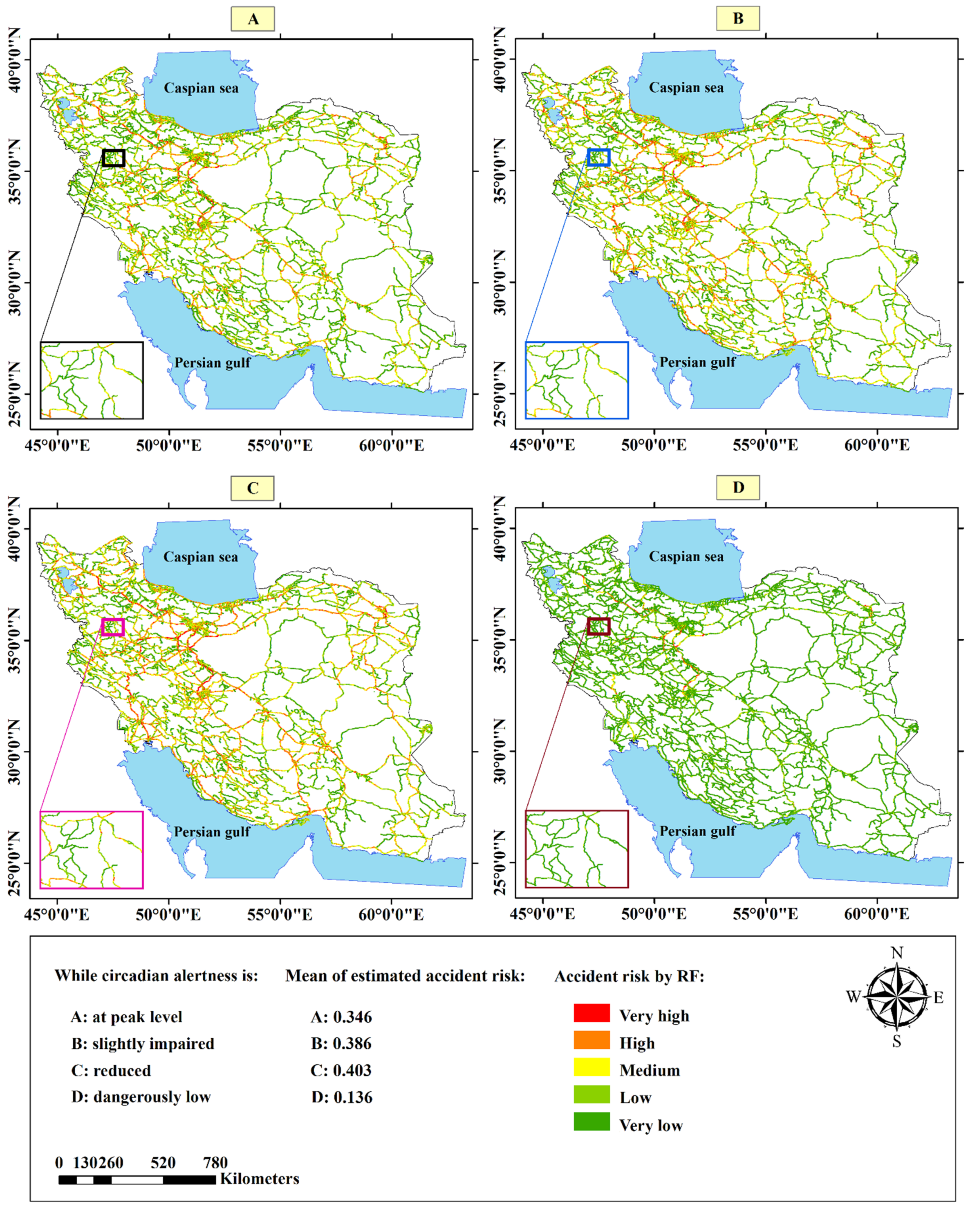
• Time of day: Time of day is an associated factor with driver alertness [65]. Accident data records were divided into four classes (Figure 3) based on a typical circadian rhythm with peak alertness at around 8:00 p.m. and 10 a.m. [77], and all classes were weighted (Table 3). The detailed classes and the number of accidents per class are listed in Table 4.
• Traffic direction: Traffic flow affects the level of driver alertness [78]. Drivers are used to getting visual information about traffic situations, and this behavior is associated with their alertness level [63]. In general, there are two types of traffic direction (one-way and two-way) that make different conditions both for traffic flow and visual traffic situations. In modeling, one-way roads were labeled 1, and two-way roads were labeled 0.
• Slope: Road geometry is significantly affected by the terrain slope. Increasing the slope makes the road geometry more varied [10]. Moreover, changing the slope make drivers careful to control their speed [45]. These led to the choice of slope as an effective criterion in modeling. The global multi-resolution terrain elevation data (GMTED 2010), with a resolution of 225 m, were used to obtain slope values.

Figure 5. Estimated spatial criteria in the study area.

Figure 5. Estimated spatial criteria in the study area.

Table 3. Detailed effective criteria in spatial modeling.

Criterion	Value/Weight
Distance to the city	Normalized in the range of [0, 1]
Distance to the gas station	Normalized in the range of [0, 1]
Land use/cover	Bare land and desert = 1 Rock, salt land, and sand dune = 0.8 Agriculture, and range = 0.6 Wetland = 0.4 Forest and shoreline = 0.2 Urban = 0
Road structure	Bridge = 1 Normal road = 0.5 Tunnel = 0
Road type	Freeway = 1 Highway = 0.65 Primary road = 0.3 Secondary road = 0
Time of day	05:00–06:00 = 1 24:00–05:00, 06:00–07:00, and 13:30–16:00 = 0.66 07:00–08:00, 10:00–13:30, 16:00–17:00, and 21:00–24:00 = 0.33 08:00–10:00, and 17:00–21:00 = 0
Traffic direction	One-way = 1 Two-way = 0
Slope	Normalized in the range of [0, 1]

Table 3. Detailed effective criteria in spatial modeling.

Criterion	Value/Weight
Distance to the city	Normalized in the range of [0, 1]
Distance to the gas station	Normalized in the range of [0, 1]
Land use/cover	Bare land and desert = 1 Rock, salt land, and sand dune = 0.8 Agriculture, and range = 0.6 Wetland = 0.4 Forest and shoreline = 0.2 Urban = 0
Road structure	Bridge = 1 Normal road = 0.5 Tunnel = 0
Road type	Freeway = 1 Highway = 0.65 Primary road = 0.3 Secondary road = 0
Time of day	05:00–06:00 = 1 24:00–05:00, 06:00–07:00, and 13:30–16:00 = 0.66 07:00–08:00, 10:00–13:30, 16:00–17:00, and 21:00–24:00 = 0.33 08:00–10:00, and 17:00–21:00 = 0
Traffic direction	One-way = 1 Two-way = 0
Slope	Normalized in the range of [0, 1]

Table 4. Detailed time classes.

Class	Time	Number of Accidents
While circadian alertness is dangerously low	05:00–06:00	203 (4.62%)
While circadian alertness is slightly impaired	24:00–05:00, 06:00–07:00, and 13:30–16:00	1684 (38.28%)
While circadian alertness is reduced	07:00–08:00, 10:00–13:30, 16:00–17:00, and 21:00–24:00	1490 (33.87%)
While circadian alertness is at peak level	08:00–10:00, and 17:00–21:00	1022 (23.23%)

Table 4. Detailed time classes.

Class	Time	Number of Accidents
While circadian alertness is dangerously low	05:00–06:00	203 (4.62%)
While circadian alertness is slightly impaired	24:00–05:00, 06:00–07:00, and 13:30–16:00	1684 (38.28%)
While circadian alertness is reduced	07:00–08:00, 10:00–13:30, 16:00–17:00, and 21:00–24:00	1490 (33.87%)
While circadian alertness is at peak level	08:00–10:00, and 17:00–21:00	1022 (23.23%)

2.4. Methods

2.4.1. Data Preprocessing

One of the preprocessing approaches in machine learning where the data are scaled or transformed to make modeling features contribute equally is normalization [79]. Before applying predictive models, using Equation (1), we normalized all features in the range of [0, 1].

$${\mathrm{X}}_{\mathrm{Normalized}}=\frac{(\mathrm{X}-{\mathrm{X}}_{\mathrm{Min}})}{({\mathrm{X}}_{\mathrm{Max}}-{\mathrm{X}}_{\mathrm{Min}})}$$

(1)

In Equation (1), X_min and X_Max are the minimum and maximum values of the feature, respectively.

2.4.2. Bagged Decision Trees Algorithm

Bagging is an ensemble machine learning algorithm that helps to enhance the unstable models’ performance when data are high-dimensional [80]. In ensemble learning, a group of estimators is used; that is, each estimator creates its data model for prediction, and at the end, samples are predicted by voting or averaging between models’ predictions [81]. Bagging can use different estimators as the base predictive model, but the decision tree is often chosen. Each algorithm is trained with a random subset of samples in this ensemble algorithm [82].

2.4.3. Extra Trees Algorithm

The decision tree is a practical machine learning algorithm [83]. This method is popular due to its high learning speed, lack of domain knowledge, interaction with multidimensional datasets, and construction of understandable models [10]. A decision tree structure is top-down, with a root, nodes, branches, and leaves [84]. The extra tree and classic decision tree are different in the way they are built. In the extra tree algorithm, to obtain the best divisions for separating the samples of a node into two groups, random splits are drawn, and the best division among them is chosen [40].

2.4.4. Random Forest Algorithm

RF is a supervised machine learning algorithm that makes its data model with ensemble learning technique. The base estimators in this ensemble algorithm are decision trees trained with randomly selected samples and sample features [85]. This learning technique has performed well in large-scale problems or where the number of variables is more than observations [86]. In RF, all trees contribute to the result, and samples are predicted by averaging or voting between trees’ predictions [10].

2.5. Validation

2.5.1. K-Fold Cross-Validation

The K-fold cross-validation method helps to understand how the prediction of a model will generalize to independent data. This method clarifies the effectiveness of a predictive model in practice [87]. K-fold subdivides the data into K subsets. One of the data subsets is utilized for validation in each iteration, while the other K-1 data subsets are used for training. This approach is made for K times; therefore, all data are used for training and validation. In the end, the average of all K validation times shows the final estimate [88].

2.5.2. Validation Metrics

The performance of three machine learning algorithms was assessed using MAE, MSE, and ROC-AUC metrics. MAE is the mean absolute error between the actual values and the estimated values. This metric is not sensitive to significant errors [10]. MAE is a suitable metric for the evaluation of average model performance. MSE equals to mean squares of errors between the actual values and the estimated values. This metric punishes outliers and does not apply mistakes with the same weight [89]. MAE and MSE are defined with Equations (2) and (3), respectively.

$$\mathrm{MAE}=\frac{1}{\mathrm{n}}{\displaystyle \sum }_{\mathrm{i}=1}^{\mathrm{n}}\left|{\mathrm{y}}_{\mathrm{i}}-\widehat{{\mathrm{y}}_{\mathrm{i}}}\right|$$

(2)

$$\mathrm{MSE}=\frac{1}{\mathrm{n}}{\displaystyle \sum }_{\mathrm{i}=1}^{\mathrm{n}}{{(\mathrm{y}}_{\mathrm{i}}-\widehat{{\mathrm{y}}_{\mathrm{i}}})}^2$$

(3)

In Equations (2) and (3), ${\mathrm{y}}_{\mathrm{i}}$ is the predicted value, $\widehat{{\mathrm{y}}_{\mathrm{i}}}$ is the actual sample value, and $\mathrm{n}$ is the number of samples.

The y-axis of the ROC curve represents sensitivity, whereas the x-axis represents specificity. The contrast between the sensitivity and specificity in several cutting points evaluates the model performance [10]. The sensitivity and specificity are probabilistic metrics in the range of [0, 1], computed using Equations (4) and (5), respectively. The probability of a correct prediction of positive and negative samples is measured by sensitivity, and specificity, respectively [90]. The area under the ROC curve is called AUC and detects the probability of a correct prediction of a random sample. AUC is in the range of [0, 1], and the higher AUC shows the better model performance [91].

$$\mathrm{Sensitivity}=\frac{\mathrm{TP}}{\mathrm{TP}+\mathrm{FN}}$$

(4)

$$\mathrm{Specificity}=\frac{\mathrm{TN}}{\mathrm{TN}+\mathrm{FP}}$$

(5)

The number of correctly predicted positive samples is TP, the number of incorrectly predicted positive samples in FP, the number of correctly predicted negative samples is TN, and the number of incorrectly predicted negative samples in FN [92].

3. Results

With the Python scikit-learn library in Anaconda software, we created BDT, ET, and RF algorithms. In this stage, according to experts, the most important hyper parameters for each algorithm were selected to be tuned by using the random search method [93] with 100 iterations.

3.1. Accident-Risk Mapping

Table 5. Calculated hyper parameters for spatial risk models.

Method	Hyper Parameters
BDT	Number of base estimators: 74	Max_features: 1
	Max_samples: 0.4694	Bootstrap: True
ET	Number of base estimators: 96	Max_features: 0.3535
	Min_samples_split: 2	Max_depth: 41
	Min_samples_leaf: 1	Bootstrap: False
	Max_samples: 1
RF	Number of base estimators: 100	Max_features: 0.3535
	Min_samples_split: 3	Max_depth: 61
	Min_samples_leaf: 1	Bootstrap: True
	Max_samples: 0.7959

shows the hyper parameters used for the optimization of BDT, ET, and RF algorithms. In this table, the base estimator is the decision tree, max_samples is the ratio of samples needed for training each tree. Moreover, max_features for BDT is the ratio of features needed for training each tree, and for ET and RF, it is the ratio of features to consider when looking for the best split. Furthermore, min_samples_split is the minimum number of samples required to split an internal node, min_samples_leaf is the minimum number of samples needed to be at a leaf node, and max_depth is the maximum depth of trees. RF used the most estimators. The minimum and the mean tree depth of this ensemble algorithm were 23 and 28.93, respectively. The number of estimators of the ET algorithm was four less than RF, and its trees often had more depth than the other two algorithms. The minimum and the mean tree depth of the ET algorithm were 27 and 31.08, respectively. BDT was made of the least estimators, and its trees usually had less depth. The maximum, minimum, and mean depth of the BDT trees were 45, 19, and 26.19, respectively.

Using the k-fold method with 5-folds, we cross-validated the predictive models. Overall, RF, ET, and BDT with slight differences had the most negligible errors, respectively. For RF, mean MAE of train data, mean MAE of test data, mean MSE of train data, and mean MSE of test data were 0.159, 0.313, 0.042, and 0.160, respectively. Based on the ET algorithm, the mean MAE of train data was 0.188, the mean MAE of test data was 0.319, the mean MSE of train data was 0.057, and the mean MSE of test data was 0.164. Correspondingly, 0.195, 0.312, 0.064, and 0.161 were similar MAE and MSE values for the BDT algorithm. Very small standard deviation (SD) values were observed for MAE and MSE values of spatial risk models. This indicated that models’ performance had no significant dependency to train and test data distribution.

Spatial prediction of accident risk caused by driver lack of alertness was performed with BDT, ET, and RF algorithms in the range of [0,1]. Very low risk (0–0.2), low risk (0.2–0.4), medium risk (0.4–0.6), high risk (0.6–0.8), and very high risk (0.8–1) were used to classify these predictions into five classes with equal intervals. Figure 6, Figure 7 and Figure 8 present the mapped accident risk by BDT, ET, and RF, respectively. Four different risk maps are given in these figures; each relates to a circadian alertness condition (Table 4). Map A, map B, map C, and map D indicate when circadian alertness is at its peak, reduced, slightly impaired, and dangerously low, respectively. In all prepared maps, the mean of estimated accident risk increases as circadian alertness goes from peak level to slightly impaired. However, the mean of calculated accident risk when circadian alertness is dangerously low is unacceptable. By merging the prepared risk maps, areas that had the highest accident risk at all times of day were identified. The Khalij Fars, Zanjan-Gahzvin, Tabriz-Zanjan, Amirkabir, Saveh-Hamedan, Tehran-Saveh, and Karaj-Ghazvin freeways had the highest accident risk in all estimated risk maps, respectively.

3.2. Identification and Prioritizing of Accident-Prone Locations

By applying the KDE on accident-risk maps, the most significant accident-prone locations were identified. Accordingly, we first merged the accident-risk maps to obtain the mean accident risk at each road point. Then we applied the KDE and classified the results into two classes with the natural junks method. Overall, 237 points were identified in the study area, as shown in Figure 9. These points must be given priority in taking the necessary steps.

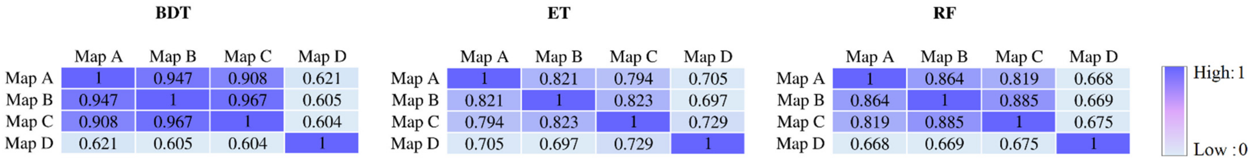
3.3. Correlation between Accident Risks at Different Times of Day

To understand how estimated accident risk changed at different times of day, the Pearson coefficient was calculated. Figure 10 shows the correlation between accident risk in four risk maps of BDT, ET, and RF models. High correlation values indicate that also time factor changes the accident risk, but it does not change the accident occurrence pattern significantly. Map D had the lowest correlations with other maps. Completely different traffic and light conditions at 05:00–06:00 compared to other times of day might cause this.

3.4. Spatial Features’ Importance

The Gini method [94] evaluated the importance of features in the spatial risk models (Figure 11). The features’ importance in these tree models was similar. Distance to the gas station (0.214), distance to the city (0.207), road type (0.200), and slope (0.199) had significantly higher scores than the average score (0.125); time (0.9) was close to the average score, and traffic direction (0.053), land use/cover (0.032), and road structure (0.005) had remarkably lowest scores.

3.5. Models Validation

Cross-validation of the study was performed with MAE, MSE, and ROC-AUC metrics. Figure 12 shows MAE and MSE values of train and test data. Although RF almost had the lowest errors, no large difference was observed in the errors of test data between all three risk models.

Using the 1760 data records and five-folds, we drew ROC graphs for cross-validation of accident-risk models (Figure 13). For plotting the ROC graphs, accident points were labeled positive (1), and other accident-free road points were labeled negative (0). The ratio of positive samples to negative samples in this cross-validation was 0.5125, 0.4790, 0.4994, 0.5011, and 0.5023, respectively. The detailed results of all ROC graphs are listed in

Table 6. Detailed results of AUC-ROC for risk models, using 5-fold validation.

Model	Fold Number	AUC	Standard Error	95% Confidence Interval	Mean AUC	SD
BDT	1	0.844	0.00906	0.826 to 0.861	0.846	0.002
	2	0.844	0.00917	0.826 to 0.860
	3	0.845	0.00904	0.828 to 0.862
	4	0.850	0.00886	0.832 to 0.866
	5	0.846	0.00906	0.828 to 0.862
ET	1	0.833	0.00937	0.815 to 0.850	0.840	0.005
	2	0.838	0.00937	0.820 to 0.855
	3	0.839	0.00918	0.821 to 0.856
	4	0.846	0.00903	0.828 to 0.862
	5	0.844	0.00913	0.826 to 0.860
RF	1	0.842	0.00912	0.824 to 0.859	0.847	0.003
	2	0.847	0.00912	0.829 to 0.863
	3	0.845	0.00907	0.827 to 0.861
	4	0.851	0.00886	0.834 to 0.868
	5	0.848	0.00899	0.830 to 0.864

.

The greatest AUC for BDT was 0.850, with a standard error of 0.00906 and a 95% confidence range of 0.826 to 0.861, according to Table 6. The highest observed AUC for ET was 0.846, with a standard error of 0.00903 and a 95% confidence interval of 0.828 to 0.862. Correspondingly, 0.851, 0.00886, and 0.834 to 0.868 were similar values for RF. On average, RF, BDT, and ET with slight differences were the most accurate models, respectively. SD values were also calculated to understand models’ accuracy to train and test data distribution. No significant dependency was observed for all models.

3.6. Evaluation of Hyper Parameters Tuning

The accuracy of BDT, ET, and RF algorithms was validated with ROC-AUC before and after hyper parameters tuning to understand the effectiveness of model optimization with the random search method.

Table 7. Detailed results of AUC-ROC for risk models, using 5-fold validation without hyper parameters tuning.

Model	Fold Number	AUC	Standard Error	95% Confidence Interval	Mean AUC	SD
BDT	1	0.825	0.00965	0.806 to 0.842	0.827	0.002
	2	0.819	0.00970	0.800 to 0.836
	3	0.841	0.00916	0.823 to 0.857
	4	0.827	0.00978	0.809 to 0.845
	5	0.832	0.00958	0.813 to 0.849
ET	1	0.842	0.00928	0.825 to 0.859	0.828	0.006
	2	0.830	0.00954	0.812 to 0.847
	3	0.825	0.00961	0.807 to 0.843
	4	0.846	0.00902	0.828 to 0.862
	5	0.828	0.00957	0.810 to 0.846
RF	1	0.830	0.00941	0.812 to 0.848	0.845	0.004
	2	0.851	0.00884	0.833 to 0.867
	3	0.826	0.00967	0.807 to 0.843
	4	0.833	0.00943	0.815 to 0.850
	5	0.846	0.00903	0.828 to 0.863

indicates the results of ROC-AUC for ensemble algorithms before hyper parameter tuning. It is clear that hyper parameters tuning improved the models’ accuracy, but improvement is not significant. It can be concluded that random search is a limited method for tuning hyper parameters, and more effective strategies should be used for this purpose.

4. Discussion

In this study, eight effective criteria were used for spatial modeling of accident risk caused by driver lack of alertness. Three ensemble-tree-based machine learning algorithms with different structures, including BDT, ET, and RF trained with actual accident points. They estimated the accident risk on Iran roads when typical circadian alertness is at peak level, reduced, slightly impaired, and dangerously low.

Based on the results derived from the ROC curves, RF, BDT, and ET algorithms with slight differences had the most accurate predictions, respectively. No significant difference between AUC values in cross-validation with five-folds for all risk models was observed. Calculated values of SD for AUC showed that created risk models had no significant dependency to train and test data distribution. The reason for the above can be found in the way how trees of each algorithm are built. Despite the RF that uses a subset of sample features for splitting a tree node and dividing samples into two groups, in the BDT, all sample features are used for this purpose. Therefore RF has a more independent structure and usually performs better than BDT [95]. Unlike BDT and RF that use the bootstrap technique for developing each decision tree, the ET algorithm fits trees on the whole samples [96]. In the ET algorithm, to create a tree node, an attempt is made to select the best feature for separating the samples into two groups [40]. Therefore, ET is tied to provide trees with more depth to cover all samples, leading to its lower accuracy and higher SD value in the cross-validation with ROC-AUC.

By describing the structure of BDT, ET, and RF algorithms, MAE and MSE values can be discussed. ET is flexible to train data and use all samples for building each tree. Therefore, its error of train data in each iteration of cross-validation was equal, and zero values of SD showed that samples’ distribution did not affect the training process of the ET algorithm. However, as BDT and RF trees do not learn with all samples, they had some errors in all iterations. In the case of test data, ET had more significant errors than BDT and RF that shows BDT and RF are more generalized to new data. Eventually, much lower MSE values than MAE indicated that no outlier was in predictions.

In general, all three algorithms performed at the same level of accuracy. It is observed in previous works that tee-based ensemble learning algorithms had almost similar performance in accident modeling [13,97]. Overall, it can be concluded that tree-based ensemble algorithms are helpful in the field of road safety analysis even when working with large-scale data, as they result in a robust prediction with reduced variance [97].

The mean of estimated accident risk in all prepared risk maps was also calculated to validate them. An acceptable rising trend was observed in all estimated risk maps when circadian alertness decreased, but while circadian alertness was dangerously low, mean accident risk was less than expected. This is because traffic volume at 05:00 to 06:00 is low, and usually, professional drivers, who can drive longer with high alertness, drive at this time of day [98,99]. This is because, only at 05:00 to 06:00, circadian alertness is considered dangerously low, and at this time of day, traffic volume is low. Low traffic volume results in low accident frequency, and since BDT, ET, and RF only learned based on the accident points data, mean accident risk at 05:00 to 06:00 was predicted to be low. However, freeways that often have high traffic volume at all hours of the day had a high level of accident risk in all prepared maps. This means driver alertness decreases more rapidly on freeways [100].

Using the estimated accident-risk maps, the most significant accident-prone locations were prioritized with KDE. Compared to previous methods that considered only the spatial density of accident points [101,102], the result of this approach is more reliable and generalizable because the accident-prone locations are obtained according to the impact of various factors on the occurrence of accidents.

On average, distance to the gas station, distance to the city, road type, slope, time of day, traffic direction, land use/cover, and road structure were the most important modeling features. Distance to the city and distance to the gas station had similar importance. In line with previous research [10], distance-based factors are often good features in modeling, as they include an extensive range of values, and driving duration is associated with distance. Besides, roadside gas stations in Iran often provide suitable facilities for drivers to rest, and this increased the importance of distance to the gas station criterion. This finding is in line with previous work, which confirmed the influence of roadside rest areas in reducing the accident risk [71]. Any road type has its design standards. Road type defines the geometric, traffic, structure, and many characteristics of the road [76], so this criterion affects a wide range of road attributes, and its high importance was expected. The slope was the next important modeling feature. In designing any road, earthworks are dependent on terrain slope [10]. Therefore, slope influences the road characteristics directly, which is an effective factor for driver alertness [64]. Alertness is controlled by the body clock and has different levels at different times of day [103]. Therefore, the time of day was an essential feature in this modeling. However, RTA frequency that affected the learning process of the created risk models is associated with traffic volume, and different traffic volume situations in times of day influenced the importance of this criterion. Traffic direction and road structure did not have a good range of values to help the predictions, and their importance obtained low. The low impact of the traffic situation on driver alertness was observed in other research, too [65]. Land use/cover was another low important modeling feature, while many land-use/cover types were observed in the study area. This observation is in line with Ahlström et al.’s [104] experimental finding that visual characteristics of road environment have little impact on driver alertness.

5. Conclusions

This study aimed to use three machine learning algorithms for spatial modeling of accident risk caused by drivers’ lack of alertness. Accident risk was mapped with BDT, ET, and RF algorithms on Iranian roads in different circadian alertness situations. The performance of created risk models was cross-validated by different metrics. Validation results showed that all three algorithms, namely BDT, ET, and RF, had similar performance and no significant difference was in their accuracy. Nevertheless, in a strict comparison, BDT had faster training due to its easier tuning, the training process of ET had less dependency to samples distribution, and RF was more accurate. The hyper parameters tuning was performed with the random search method and increased the accuracy of machine learning algorithms slightly. It is recommended that the effectiveness of other optimization methods on accident-risk modeling be investigated in future works.

The mean estimated accident risk in different circadian alertness situations was investigated. It can be said that traffic volume was the limitation of this study. Contrary to what was expected, dangerously low alertness at 05:00 to 06:00 did not result in higher accident risk due to special traffic conditions. As a result, RTA risk modeling using accident points without normalization of accident frequency with traffic volume might decrease the quality of prediction and features’ importance evaluation.

Freeways are identified as the riskiest road types when the driver is not alert. The risk of accidents on freeways was predicted to be high at all times of day, and Khalij Fars, Zanjan-Gahzvin, Tabriz-Zanjan, Amirkabir, Saveh-Hamedan, Tehran-Saveh, and Karaj-Ghazvin freeways had the highest estimated accident risk, respectively. In general, risk mapping of RTA by clarifying the impact of different factors on road safety, identifying risky areas, and prioritizing accident-prone locations can help decision-makers to take necessary actions.

References

1. WHO Global Status Report on Road Safety 2018. Available online: https://www.who.int/publications-detail/global-status-report-on-road-safety-2018 (accessed on 17 June 2018).
2. Bhalla, K.; Naghavi, M.; Shahraz, S.; Bartels, D.; Murray, C.J. Building national estimates of the burden of road traffic injuries in developing countries from all available data sources: Iran. Inj. Prev. 2009, 15, 150–156. [Google Scholar] [CrossRef] [Green Version]
3. IRMTO Statistical Yearbook of the Road Maintenance and Transportation Organization 2020. Available online: http://rmto.ir/Pages/SalnameAmari.aspx (accessed on 16 February 2021).
4. Behnood, H.R.; Haddadi, M.; Sirous, S.; Ainy, E.; Rezaei, R. Medical costs and economic burden caused by road traffic injuries in Iran. Trauma Mon. 2017, 22. [Google Scholar] [CrossRef] [Green Version]
5. Sargazi, A.; Sargazi, A.; Jim, P.K.N.; Danesh, H.; Aval, F.; Kiani, Z.; Lashkarinia, A.; Sepehri, Z. Economic burden of road traffic accidents; report from a single center from south Eastern Iran. Bull. Emerg. Trauma 2016, 4, 43. [Google Scholar]
6. Gorea, R. Financial impact of road traffic accidents on the society. Int. J. Ethics Trauma Vict. 2016, 2, 6–9. [Google Scholar] [CrossRef]
7. Lee, J.; Chae, J.; Yoon, T.; Yang, H. Traffic accident severity analysis with rain-related factors using structural equation modeling—A case study of Seoul City. Accid. Anal. Prev. 2018, 112, 1–10. [Google Scholar] [CrossRef] [PubMed]
8. Hazaa, M.A.; Saad, R.M.; Alnaklani, M.A. Prediction of Traffic Accident Severity using Data Mining Techniques in IBB Province, Yemen. Int. J. Softw. Eng. Comput. Syst. 2019, 5, 77–92. [Google Scholar] [CrossRef]
9. Chen, M.-M.; Chen, M.-C. Modeling road accident severity with comparisons of logistic regression, decision tree and random forest. Information 2020, 11, 270. [Google Scholar] [CrossRef]
10. Farhangi, F.; Sadeghi-Niaraki, A.; Nahvi, A.; Razavi-Termeh, S.V. Spatial modeling of accidents risk caused by driver drowsiness with data mining algorithms. Geocarto Int. 2020, 1–15. [Google Scholar] [CrossRef]
11. Driss, M.; Benabdeli, K.; Saint-Gerand, T.; Hamadouche, M. Traffic safety prediction model for identifying spatial degrees of exposure to the risk of road accidents based on fuzzy logic approach. Geocarto Int. 2015, 30, 243–257. [Google Scholar] [CrossRef]
12. Bhowmik, T.; Yasmin, S.; Eluru, N. Do we need multivariate modeling approaches to model crash frequency by crash types? A panel mixed approach to modeling crash frequency by crash types. Anal. Methods Accid. Res. 2019, 24, 100107. [Google Scholar] [CrossRef]
13. Zhang, X.; Waller, S.T.; Jiang, P. An ensemble machine learning-based modeling framework for analysis of traffic crash frequency. Comput.-Aided Civ. Infrastruct. Eng. 2020, 35, 258–276. [Google Scholar] [CrossRef]
14. Al-Radaideh, Q.A.; Daoud, E.J. Data mining methods for traffic accident severity prediction. Int. J. Neural Netw. Adv. Appl. 2018, 5, 1–12. [Google Scholar]
15. Erdogan, S.; Yilmaz, I.; Baybura, T.; Gullu, M. Geographical information systems aided traffic accident analysis system case study: City of Afyonkarahisar. Accid. Anal. Prev. 2008, 40, 174–181. [Google Scholar] [CrossRef] [PubMed]
16. El Naqa, I.; Murphy, M.J. What is machine learning? In Machine Learning in Radiation Oncology; Springer: Berlin/Heidelberg, Germany, 2015; pp. 3–11. [Google Scholar]
17. Yang, L.; Shami, A. On hyperparameter optimization of machine learning algorithms: Theory and practice. Neurocomputing 2020, 415, 295–316. [Google Scholar] [CrossRef]
18. Witten, I.H.; Frank, E. Data mining: Practical machine learning tools and techniques with Java implementations. Acm Sigmod Rec. 2002, 31, 76–77. [Google Scholar] [CrossRef]
19. Ardabili, S.; Mosavi, A.; Várkonyi-Kóczy, A.R. Advances in Machine Learning Modeling Reviewing Hybrid and Ensemble. In Engineering for Sustainable Future; Springer: Berlin/Heidelberg, Germany, 2019; pp. 215–227. [Google Scholar]
20. Hegde, J.; Rokseth, B. Applications of machine learning methods for engineering risk assessment—A review. Saf. Sci. 2020, 122, 104492. [Google Scholar] [CrossRef]
21. Al-Dogom, D.; Aburaed, N.; Al-Saad, M.; Almansoori, S. Spatio-temporal analysis and machine learning for traffic accidents prediction. In Proceedings of the 2019 2nd International Conference on Signal Processing and Information Security (ICSPIS), Dubai, UAE, 30–31 October 2019; IEEE: Piscataway, NJ, USA, 2019; pp. 1–4. [Google Scholar]
22. Wang, C.; Liu, L.; Xu, C.; Lv, W. Predicting future driving risk of crash-involved drivers based on a systematic machine learning framework. Int. J. Environ. Res. Public Health 2019, 16, 334. [Google Scholar] [CrossRef] [PubMed] [Green Version]
23. Ziakopoulos, A.; Yannis, G. A review of spatial approaches in road safety. Accid. Anal. Prev. 2020, 135, 105323. [Google Scholar] [CrossRef]
24. Silva, P.B.; Andrade, M.; Ferreira, S. Machine learning applied to road safety modeling: A systematic literature review. J. Traffic Transp. Eng. 2020, 7, 775–790. [Google Scholar]
25. Lee, J.; Yoon, T.; Kwon, S.; Lee, J. Model evaluation for forecasting traffic accident severity in rainy seasons using machine learning algorithms: Seoul city study. Appl. Sci. 2020, 10, 129. [Google Scholar] [CrossRef] [Green Version]
26. Mestri, R.A.; Rathod, R.R.; Garg, R.D. Identification and removal of accident-prone locations using spatial data mining. In Applications of Geomatics in Civil Engineering; Springer: Berlin/Heidelberg, Germany, 2020; pp. 383–394. [Google Scholar]
27. Fan, Z.; Liu, C.; Cai, D.; Yue, S. Research on black spot identification of safety in urban traffic accidents based on machine learning method. Saf. Sci. 2019, 118, 607–616. [Google Scholar] [CrossRef]
28. Rovšek, V.; Batista, M.; Bogunović, B. Identifying the key risk factors of traffic accident injury severity on Slovenian roads using a non-parametric classification tree. Transport 2017, 32, 272–281. [Google Scholar] [CrossRef] [Green Version]
29. Taamneh, M.; Alkheder, S.; Taamneh, S. Data-mining techniques for traffic accident modeling and prediction in the United Arab Emirates. J. Transp. Saf. Secur. 2017, 9, 146–166. [Google Scholar] [CrossRef]
30. Kumar, S.; Toshniwal, D. A data mining approach to characterize road accident locations. J. Mod. Transp. 2016, 24, 62–72. [Google Scholar] [CrossRef] [Green Version]
31. Tao, G.; Song, H.; Liu, J.; Zou, J.; Chen, Y. A traffic accident morphology diagnostic model based on a rough set decision tree. Transp. Plan. Technol. 2016, 39, 751–758. [Google Scholar] [CrossRef]
32. Zeng, Q.; Huang, H.; Pei, X.; Wong, S.; Gao, M. Rule extraction from an optimized neural network for traffic crash frequency modeling. Accid. Anal. Prev. 2016, 97, 87–95. [Google Scholar] [CrossRef] [PubMed] [Green Version]
33. Wang, J.; Zheng, Y.; Li, X.; Yu, C.; Kodaka, K.; Li, K. Driving risk assessment using near-crash database through data mining of tree-based model. Accid. Anal. Prev. 2015, 84, 54–64. [Google Scholar] [CrossRef] [PubMed]
34. Beshah, T.; Ejigu, D.; Abraham, A.; Snasel, V.; Kromer, P. Pattern recognition and knowledge discovery from road traffic accident data in ethiopia: Implications for improving road safety. In Proceedings of the 2011 World Congress on Information and Communication Technologies, Mumbai, India, 11–14 December 2011; pp. 1241–1246. [Google Scholar]
35. Das, A.; Abdel-Aty, M.A. A combined frequency–severity approach for the analysis of rear-end crashes on urban arterials. Saf. Sci. 2011, 49, 1156–1163. [Google Scholar] [CrossRef]
36. Chang, L.-Y.; Chen, W.-C. Data mining of tree-based models to analyze freeway accident frequency. J. Saf. Res. 2005, 36, 365–375. [Google Scholar] [CrossRef] [PubMed]
37. Sagi, O.; Rokach, L. Ensemble learning: A survey. Wiley Interdiscip. Rev. Data Min. Knowl. Discov. 2018, 8, e1249. [Google Scholar] [CrossRef]
38. Hegde, C.; Wallace, S.; Gray, K. Using Trees, Bagging, and Random Forests to Predict Rate of Penetration During Drilling. In Proceedings of the SPE Middle East Intelligent Oil and Gas Conference and Exhibition, Abu Dhabi, United Arab Emirates, 15–16 September 2015; Society of Petroleum Engineers: Denver, CO, USA, 2015. [Google Scholar]
39. Lee, T.-H.; Ullah, A.; Wang, R. Bootstrap aggregating and random forest. In Macroeconomic Forecasting in the Era of Big Data; Springer: Berlin/Heidelberg, Germany, 2020; pp. 389–429. [Google Scholar]
40. Geurts, P.; Ernst, D.; Wehenkel, L. Extremely randomized trees. Mach. Learn. 2006, 63, 3–42. [Google Scholar] [CrossRef] [Green Version]
41. Shahzad, M. Review of road accident analysis using GIS technique. Int. J. Inj. Control. Saf. Promot. 2020, 27, 472–481. [Google Scholar] [CrossRef]
42. Kumar, D.; Singh, R.; Kaur, R. GIS Databases: Spatial and Non-spatial. In Spatial Information Technology for Sustainable Development Goals; Springer: Berlin/Heidelberg, Germany, 2019; pp. 15–25. [Google Scholar]
43. Budzyński, M.; Kustra, W.; Okraszewska, R.; Jamroz, K.; Pyrchla, J. The Use of GIS Tools for Road Infrastructure Safety Management. In E3S Web of Conferences; EDP Sciences: Ulis, France, 2018; p. 00009. [Google Scholar]
44. Le, K.G.; Liu, P.; Lin, L.-T. Determining the road traffic accident hotspots using GIS-based temporal-spatial statistical analytic techniques in Hanoi, Vietnam. Geo-Spat. Inf. Sci. 2020, 23, 153–164. [Google Scholar] [CrossRef] [Green Version]
45. Naboureh, A.; Feizizadeh, B.; Naboureh, A.; Bian, J.; Blaschke, T.; Ghorbanzadeh, O.; Moharrami, M. Traffic Accident Spatial Simulation Modeling for Planning of Road Emergency Services. Int. J. Geo-Inf. 2019, 8, 371. [Google Scholar] [CrossRef] [Green Version]
46. Briz-Redón, Á.; Mateu, J.; Montes, F. Modeling accident risk at the road level through zero-inflated negative binomial models: A case study of multiple road networks. Spat. Stat. 2021, 43, 100503. [Google Scholar] [CrossRef]
47. Prasannakumar, V.; Vijith, H.; Charutha, R.; Geetha, N. Spatio-temporal clustering of road accidents: GIS based analysis and assessment. Procedia-Soc. Behav. Sci. 2011, 21, 317–325. [Google Scholar] [CrossRef] [Green Version]
48. Shafabakhsh, G.A.; Famili, A.; Bahadori, M.S. GIS-based spatial analysis of urban traffic accidents: Case study in Mashhad, Iran. J. Traffic Transp. Eng. 2017, 4, 290–299. [Google Scholar] [CrossRef]
49. Owusu, C.K.; Eshun, J.K.; Asare, C.K.O.; Aikins, A.A. Identification of Road Traffic Accident Hotspots in the Cape Coast Metropolis, Southern Ghana Using Geographic Information System (GIS). Int. J. Sci. Eng. Res. 2018, 10, 2106–2123. [Google Scholar] [CrossRef]
50. Almoshaogeh, M.; Abdulrehman, R.; Haider, H.; Alharbi, F.; Jamal, A.; Alarifi, S.; Shafiquzzaman, M. Traffic Accident Risk Assessment Framework for Qassim, Saudi Arabia: Evaluating the Impact of Speed Cameras. Appl. Sci. 2021, 11, 6682. [Google Scholar] [CrossRef]
51. Aghajani, M.A.; Dezfoulian, R.S.; Arjroody, A.R.; Rezaei, M. Applying GIS to Identify the Spatial and Temporal Patterns of Road Accidents Using Spatial Statistics (case study: Ilam Province, Iran). Transp. Res. Procedia 2017, 25, 2126–2138. [Google Scholar] [CrossRef]
52. Singh, D.; Mohan, C.K. Deep spatio-temporal representation for detection of road accidents using stacked autoencoder. IEEE Trans. Intell. Transp. Syst. 2018, 20, 879–887. [Google Scholar] [CrossRef]
53. Quddus, M. Exploring the relationship between average speed, speed variation, and accident rates using spatial statistical models and GIS. J. Transp. Saf. Secur. 2013, 5, 27–45. [Google Scholar] [CrossRef]
54. Sameen, M.I.; Pradhan, B. Assessment of the effects of expressway geometric design features on the frequency of accident crash rates using high-resolution laser scanning data and GIS. Geomat. Nat. Hazards Risk 2017, 8, 733–747. [Google Scholar] [CrossRef] [Green Version]
55. Heydari, S.T.; Sarikhani, Y.; Moafian, G.; Aghabeigi, M.R.; Mahmoodi, M.; Ghaffarpasand, F.; Riasati, A.; Peymani, P.; Ahmadi, S.M.; Lankarani, K.B. Time analysis of fatal traffic accidents in Fars Province of Iran. Chin. J. Traumatol. 2013, 16, 84–88. [Google Scholar] [PubMed]
56. Sadeghi-Bazargani, H.; Ayubi, E.; Azami-Aghdash, S.; Abedi, L.; Zemestani, A.; Amanati, L.; Moosazadeh, M.; Syedi, N.; Safiri, S. Epidemiological Patterns of Road Traffic Crashes During the Last Two Decades in Iran: A Review of the Literature from 1996 to 2014. Arch. Trauma Res. 2016, 5, e32985. [Google Scholar] [CrossRef] [PubMed] [Green Version]
57. Afolabi, S.; Warrie, W.; Banjo, O.; Iwashokun, O.; Olawale, A.; Ngqambela, N.; Soliu, F.; Olasunkanmi, O.; Sakinat, F.; Matshika, S. When and where? Proactively predicting traffic accident in South Africa: Our machine learning competition winning approach. Int. J. Soc. Syst. Sci. 2021, 13, 151–170. [Google Scholar] [CrossRef]
58. Al-Aamri, A.K.; Hornby, G.; Zhang, L.-C.; Al-Maniri, A.A.; Padmadas, S.S. Mapping road traffic crash hotspots using GIS-based methods: A case study of Muscat Governorate in the Sultanate of Oman. Spat. Stat. 2021, 42, 100458. [Google Scholar] [CrossRef]
59. Roland, J.; Way, P.D.; Firat, C.; Doan, T.-N.; Sartipi, M. Modeling and predicting vehicle accident occurrence in Chattanooga, Tennessee. Accid. Anal. Prev. 2021, 149, 105860. [Google Scholar] [CrossRef]
60. Liu, J. Large-Scale Traffic Accident Data Classification Method Based on XGBoost. Des. Eng. 2020, 2020, 572–584. [Google Scholar]
61. Zahid, M.; Chen, Y.; Jamal, A.; Al-Ofi, K.A.; Al-Ahmadi, H.M. Adopting machine learning and spatial analysis techniques for driver risk assessment: Insights from a case study. Int. J. Environ. Res. Public Health 2020, 17, 5193. [Google Scholar] [CrossRef]
62. Zhu, H.; Zhou, Y.; Chen, Y. Identification of potential traffic accident hot spots based on accident data and GIS. In MATEC Web of Conferences; EDP Sciences: Ulis, France, 2020; p. 01005. [Google Scholar]
63. Pastor, G.; Tejero, P.; Choliz, M.; Roca, J. Rear-view mirror use, driver alertness and road type: An empirical study using EEG measures. Transp. Res. Part F Traffic Psychol. Behav. 2006, 9, 286–297. [Google Scholar] [CrossRef]
64. Thiffault, P.; Bergeron, J. Monotony of road environment and driver fatigue: A simulator study. Accid. Anal. Prev. 2003, 35, 381–391. [Google Scholar] [CrossRef]
65. Otmani, S.; Rogé, J.; Muzet, A. Sleepiness in professional drivers: Effect of age and time of day. Accid. Anal. Prev. 2005, 37, 930–937. [Google Scholar] [CrossRef]
66. Otmani, S.; Pebayle, T.; Roge, J.; Muzet, A. Effect of driving duration and partial sleep deprivation on subsequent alertness and performance of car drivers. Physiol. Behav. 2005, 84, 715–724. [Google Scholar] [CrossRef]
67. Smith, P.; Shah, M.; Lobo, N.d.V. Monitoring head/eye motion for driver alertness with one camera. In Proceedings of the 15th International Conference on Pattern Recognition. ICPR-2000, Barcelona, Spain, 3–7 September 2000; Volume 4, pp. 636–642. [Google Scholar]
68. Richardson, J.H. The development of a driver alertness monitoring system. In Fatigue and Driving; Routledge: London, UK, 2019; pp. 219–229. [Google Scholar]
69. Murthy, K.; Khan, Z.A. Different techniques to quantify the driver alertness. World Appl. Sci. J. 2013, 22, 1094–1098. [Google Scholar]
70. Moafian, G.; Aghabeigi, M.R.; Hoseinzadeh, A.; Lankarani, K.B.; Sarikhani, Y.; Heydari, S.T. An epidemiologic survey of road traffic accidents in Iran: Analysis of driver-related factors. Chin. J. Traumatol. 2013, 16, 140–144. [Google Scholar] [PubMed]
71. Jung, S.; Joo, S.; Oh, C. Evaluating the effects of supplemental rest areas on freeway crashes caused by drowsy driving. Accid. Anal. Prev. 2017, 99, 356–363. [Google Scholar] [CrossRef]
72. Hu, D.; Feng, X.; Zhao, X.; Li, H.; Ma, J.; Fu, Q. Impact of HMI on driver’s distraction on a freeway under heavy foggy condition based on visual characteristics. J. Transp. Saf. Secur. 2020, 1–24. [Google Scholar] [CrossRef]
73. Jiang, X.; Abdel-Aty, M.; Hu, J.; Lee, J. Investigating macro-level hotzone identification and variable importance using big data: A random forest models approach. Neurocomputing 2016, 181, 53–63. [Google Scholar] [CrossRef]
74. SCI Population and Housing Censuses 2016. Available online: https://www.amar.org.ir/english/Population-and-Housing-Censuses (accessed on 17 August 2018).
75. Ehsani Sohi, M.; Dashtestaninejad, H.; Khademi, E. Effects of Roadway and Traffic Characteristics on Accidents Frequency at City Entrance Zone. Int. J. Transp. Eng. 2019, 7, 139–152. [Google Scholar]
76. PBO Highway Geometric Design Code (No.415) of Iran. Available online: https://sama.mporg.ir/sites/Publish/en/Pages/ZabetehAllItems.aspx (accessed on 19 July 2021).
77. Gartenberg, D. The Circadian Rhythm and How to Hack Yours. Available online: https://medium.com/@dangartenberg/the-circadian-rhythm-and-how-to-hack-yours-bd8413e0aacf (accessed on 12 May 2018).
78. D’Anna, C.; Bibbo, D.; Bertollo, M.; di Fronso, S.; Comani, S.; De Blasiis, M.R.; Veraldi, V.; Goffredo, M.; Conforto, S. State of alertness during simulated driving tasks. In Proceedings of the XIV Mediterranean Conference on Medical and Biological Engineering and Computing, Paphos, Cyprus, 31 March–2 April 2016; Springer: Berlin/Heidelberg, Germany, 2016; pp. 913–918. [Google Scholar]
79. Singh, D.; Singh, B. Investigating the impact of data normalization on classification performance. Appl. Soft Comput. 2020, 97, 105524. [Google Scholar] [CrossRef]
80. Bühlmann, P.; Yu, B. Analyzing bagging. Ann. Stat. 2002, 30, 927–961. [Google Scholar] [CrossRef]
81. Dietterich, T.G. Ensemble methods in machine learning. In Multiple Classifier Systems, Proceedings of the International Workshop on Multiple Classifier Systems, Cagliari, Italy, 21–23 June 2000; Springer: Berlin/Heidelberg, Germany, 2000; pp. 1–15. [Google Scholar]
82. Razavi-Termeh, S.V.; Sadeghi-Niaraki, A.; Choi, S.-M. Spatial modeling of asthma-prone areas using remote sensing and ensemble machine learning algorithms. Remote. Sens. 2021, 13, 3222. [Google Scholar] [CrossRef]
83. Teli, S.; Kanikar, P. A survey on decision tree based approaches in data mining. Int. J. Adv. Res. Comput. Sci. Softw. Eng. 2015, 5, 613–617. [Google Scholar]
84. Sharma, H.; Kumar, S. A survey on decision tree algorithms of classification in data mining. Int. J. Sci. Res. 2016, 5, 2094–2097. [Google Scholar]
85. Razavi-Termeh, S.V.; Sadeghi-Niaraki, A.; Choi, S.-M. Effects of air pollution in spatio-temporal modeling of asthma-prone areas using a machine learning model. Environ. Res. 2021, 200, 111344. [Google Scholar] [CrossRef] [PubMed]
86. Razavi-Termeh, S.V.; Sadeghi-Niaraki, A.; Choi, S.-M. Asthma-prone areas modeling using a machine learning model. Sci. Rep. 2021, 11, 1–16. [Google Scholar] [CrossRef] [PubMed]
87. Anguita, D.; Ghelardoni, L.; Ghio, A.; Oneto, L.; Ridella, S. The ‘K’in K-fold cross validation. In Proceedings of the 20th European Symposium on Artificial Neural Networks, Computational Intelligence and Machine Learning (ESANN), Bruges, Belgium, 25–27 April 2012; pp. 441–446. [Google Scholar]
88. Fushiki, T. Estimation of prediction error by using K-fold cross-validation. Stat. Comput. 2011, 21, 137–146. [Google Scholar] [CrossRef]
89. Razavi-Termeh, S.V.; Khosravi, K.; Sadeghi-Niaraki, A.; Choi, S.-M.; Singh, V.P. Improving groundwater potential mapping using metaheuristic approaches. Hydrol. Sci. J. 2020, 65, 2729–2749. [Google Scholar] [CrossRef]
90. Xu-hui, W.; Ping, S.; Li, C.; Ye, W. A ROC curve method for performance evaluation of support vector machine with optimization strategy. In Proceedings of the 2009 International Forum on Computer Science-Technology and Applications, Chongqing, China, 25–27 December 2009; IEEE: Piscataway, NJ, USA, 2009; pp. 117–120. [Google Scholar]
91. Ranjgar, B.; Razavi-Termeh, S.V.; Foroughnia, F.; Sadeghi-Niaraki, A.; Perissin, D. Land subsidence susceptibility mapping using persistent scatterer sar interferometry technique and optimized hybrid machine learning algorithms. Remote. Sens. 2021, 13, 1326. [Google Scholar] [CrossRef]
92. Shogrkhodaei, S.Z.; Razavi-Termeh, S.V.; Fathnia, A. Spatio-temporal modeling of pm2. 5 risk mapping using three machine learning algorithms. Environ. Pollut. 2021, 289, 117859. [Google Scholar] [CrossRef] [PubMed]
93. Bergstra, J.; Bengio, Y. Random search for hyper-parameter optimization. J. Mach. Learn. Res. 2012, 13, 281–305. [Google Scholar]
94. Menze, B.H.; Kelm, B.M.; Masuch, R.; Himmelreich, U.; Bachert, P.; Petrich, W.; Hamprecht, F.A. A comparison of random forest and its Gini importance with standard chemometric methods for the feature selection and classification of spectral data. BMC Bioinform. 2009, 10, 1–16. [Google Scholar] [CrossRef] [Green Version]
95. Altman, N.; Krzywinski, M. Points of Significance: Ensemble Methods: Bagging and Random Forests; Nature Publishing Group: Berlin, Germany, 2017. [Google Scholar]
96. Brownlee, J. How to Develop an Extra Trees Ensemble with Python. Available online: https://machinelearningmastery.com/extra-trees-ensemble-with-python/ (accessed on 12 September 2021).
97. Schlögl, M. A multivariate analysis of environmental effects on road accident occurrence using a balanced bagging approach. Accid. Anal. Prev. 2020, 136, 105398. [Google Scholar] [CrossRef]
98. Noce, F.; Tufik, S.; Mello, M.T.D. Professional drivers and working time: Journey span, rest, and accidents. Sleep Sci. 2008, 1, 20–26. [Google Scholar]
99. Anund, A.; Ahlström, C.; Fors, C.; Åkerstedt, T. Are professional drivers less sleepy than non-professional drivers? Scand. J. Work. Environ. Health 2018, 44, 88–95. [Google Scholar] [CrossRef]
100. Wang, J.; Sun, S.; Fang, S.; Fu, T.; Stipancic, J. Predicting drowsy driving in real-time situations: Using an advanced driving simulator, accelerated failure time model, and virtual location-based services. Accid. Anal. Prev. 2017, 99, 321–329. [Google Scholar] [CrossRef]
101. Xie, Z.; Yan, J. Detecting traffic accident clusters with network kernel density estimation and local spatial statistics: An integrated approach. J. Transp. Geogr. 2013, 31, 64–71. [Google Scholar] [CrossRef]
102. Le, K.G.; Liu, P.; Lin, L.-T. Traffic accident hotspot identification by integrating kernel density estimation and spatial autocorrelation analysis: A case study. Int. J. Crashworthiness 2020, 1–11. [Google Scholar] [CrossRef]
103. Foster, R.G.; Kreitzman, L. The rhythms of life: What your body clock means to you! Exp. Physiol. 2014, 99, 599–606. [Google Scholar] [CrossRef]
104. Ahlström, C.; Anund, A.; Fors, C.; Åkerstedt, T. Effects of the road environment on the development of driver sleepiness in young male drivers. Accid. Anal. Prev. 2018, 112, 127–134. [Google Scholar] [CrossRef] [PubMed]
Figure 1. Research methodology.
Sustainability 13 10239 g001
Figure 2. Location map of the study area.
Sustainability 13 10239 g002
Figure 3. Distribution map of the research data records used for training and cross-validation.
Sustainability 13 10239 g003
Figure 4. Classification map of the number of accidents per Iran province (up) and distribution map of accident points for top four regions with the most accident points (down).
Sustainability 13 10239 g004
Figure 6. Estimated accident-risk maps, using BDT algorithm.
Sustainability 13 10239 g006
Figure 7. Estimated accident-risk maps, using ET algorithm.
Sustainability 13 10239 g007
Figure 8. Estimated accident-risk maps, using RF algorithm.
Sustainability 13 10239 g008
Figure 9. Most significant risky accident-prone locations in the study area.
Sustainability 13 10239 g009
Figure 10. Calculated Person coefficient between estimated accident risk at different times of day.
Sustainability 13 10239 g010
Figure 11. Features’ importance in spatial risk models.
Sustainability 13 10239 g011
Figure 12. Cross-validation of risk models by MAE and MSE of train and test data.
Sustainability 13 10239 g012
Figure 13. Validation of risk models by AUC-ROC, using 5-fold validation.
Sustainability 13 10239 g013