Article

Gully Erosion Susceptibility Assessment in the Kondoran Watershed Using Machine Learning Algorithms and the Boruta Feature Selection

by
Hamed Ahmadpour
1,
Ommolbanin Bazrafshan
1,
Elham Rafiei-Sardooi
2,
Hossein Zamani
3 and
Thomas Panagopoulos
4,*
1
Department of Natural Resources Engineering, Faculty of Agriculture and Natural Resources Engineering, University of Hormozgan, Bandar Abbas 7916193145, Iran
2
Department of Ecological Engineering, Faculty of Natural Resources, University of Jiroft, Kerman 7867161167, Iran
3
Department of Mathematics and Statistics, Faculty of Science, University of Hormozgan, Bandar Abbas 7916193145, Iran
4
Research Center for Spatial and Organizational Dynamics, University of Algarve, Gambelas Campus, 8005 Faro, Portugal
*
Author to whom correspondence should be addressed.
Sustainability 2021, 13(18), 10110; https://doi.org/10.3390/su131810110
Submission received: 28 June 2021 / Revised: 2 September 2021 / Accepted: 3 September 2021 / Published: 9 September 2021

Abstract

:
Gully erosion susceptibility mapping is an essential land management tool to reduce soil erosion damages. This study investigates gully susceptibility based on multiple diagnostic analysis, support vector machine and random forest algorithms, and also a combination of these models, namely the ensemble model. Thus, a gully susceptibility map in the Kondoran watershed of Iran was generated by applying these models on the occurrence and non-occurrence points (as the target variable) and several predictors (slope, aspect, elevation, topographic wetness index, drainage density, plan curvature, distance to streams, lithology, soil texture and land use). The Boruta algorithm was used to select the most effective variables in modeling gully erosion susceptibility. The area under the receiver operating characteristic curve (AUC), the receiver operating characteristics, and true skill statistics (TSS) were used to assess the model performance. The results indicated that the ensemble model had the best performance (AUC = 0.982, TSS = 0.93) compared to the others. The most effective factors in gully erosion susceptibility mapping of the study region were topological, anthropogenic, and geological. The methodology and variables of this study can be used in other regions to control and mitigate the gully erosion phenomenon by applying biophilic and regenerative techniques at the locations of the most influential factors.

1. Introduction

Gully erosion is the most destructive type of water erosion, commonly occurring in arid and semi-arid regions. Gully erosion is considered when the cross-section of the erosion channel is greater than 929 cm2 [1]. Gullies are usually created on plain and plateau areas depending on several factors such as land use, soil type, lithology, topography and vegetation cover [2,3]. Gullies are the most destructive type of water erosion, and have many effects such as land degradation, reduced soil fertility, and damage to infrastructures [4]. Generally, gullies were observed more in semi-arid and arid regions of Iran. A study of gully data in Iran indicated that the average length and depth of gullies in Iran were about 570 m and 2.8 m, respectively, which produced 21 m3/m sediment per unit gully length [5]. To this end, the assessment of the gully erosion status is necessary to mitigate its destructive effects in Iran and other countries. Application of physically-based soil erosion models and machine learning methods are used for investigating and modeling soil erosion [6].
Several authors have applied physically-based models such as AGNPS (Agricultural Non-point Source model) [7]; LISEM (Limburg Soil Erosion Model) [8] and RUSLE (Revised Universal Soil Loss Equation) [9,10,11] to determine soil erosion status. However, these models are complicated and large data sets are needed. In contrast, the remote sensing data, such as synthetic aperture radar (SAR), light detection and ranging (LiDAR), Quickbird, Landsat, SPOT 5, Google Earth, etc., with the aid of geographic information system (GIS) tools, provide evidence for detecting gully erosion and hazard modeling in regions with limited data [12,13,14,15,16]. The list of abbreviations is included in Appendix A Table A1.
Currently, GIS-based machine learning techniques are used for gully erosion susceptibility mapping [17]. In several studies, data mining approaches, including support vector machine (SVM) [18], random forest (RF) [19], maximum entropy (MaxEnt) [20], Generalized Linear Model (GLM) [21] with the aid of the remote sensing data and GIS tools have been applied to study gull erosion susceptibility. The SVM model can be generalized in terms of linear and non-linear kernels to avoid over-fitting. However, the SVM model cannot be used to determine the importance of predictor variables. In this regard, the importance of predictor variables on gully erosion can be obtained using the MDA model [22]. However, the assumption of normality of each predictor variable is one of the limitations of the MDA model [23]. On the other hand, the RF model is insensitive to outliers and over-fitting, and can handle multiple input variables without needing variables deletion [24].
Each of these models contains specific weaknesses in modeling gully susceptibility mapping, which can be resolved using the ensemble modeling method [25]. Generally, in previous studies, individual models were applied for gully erosion susceptibility analysis, while few studies considered ensemble models [25,26]. Therefore, testing the ensemble model as the combination of individuals to compare its performance versus the SVM, RF and MDA models in gully erosion susceptibility mapping (GESM) must be investigated. Further, in previous studies, the importance of conditioning factors was obtained using susceptibility models. In contrast, the Boruta variable selection algorithm might extract the most important predictors [27].
In the Kondoran plain region (especially in the Kondoran and Armak villages), gully erosion resulted from the sensitive soil, poor quality of downstream lands caused by flooding through salt domes, wind, and water erosion, as well as many years of unprincipled management. Although this destructive erosion already existed in the region, its expansion rate has increased dramatically in recent years. Therefore, identifying vulnerable areas to gully erosion will help to reduce land degradation. Process-oriented and stochastic models using GIS might be helpful to detect gullies and map gully erosion vulnerability.
Therefore, this study aimed to investigate the SVM, MDA and RF models approach for mapping gully susceptibility, select the most important features using the Boruta variable selection algorithm, and employ an ensemble modeling method to produce a gully susceptibility map and compare it with individual models’ performance.

2. Material and Methods
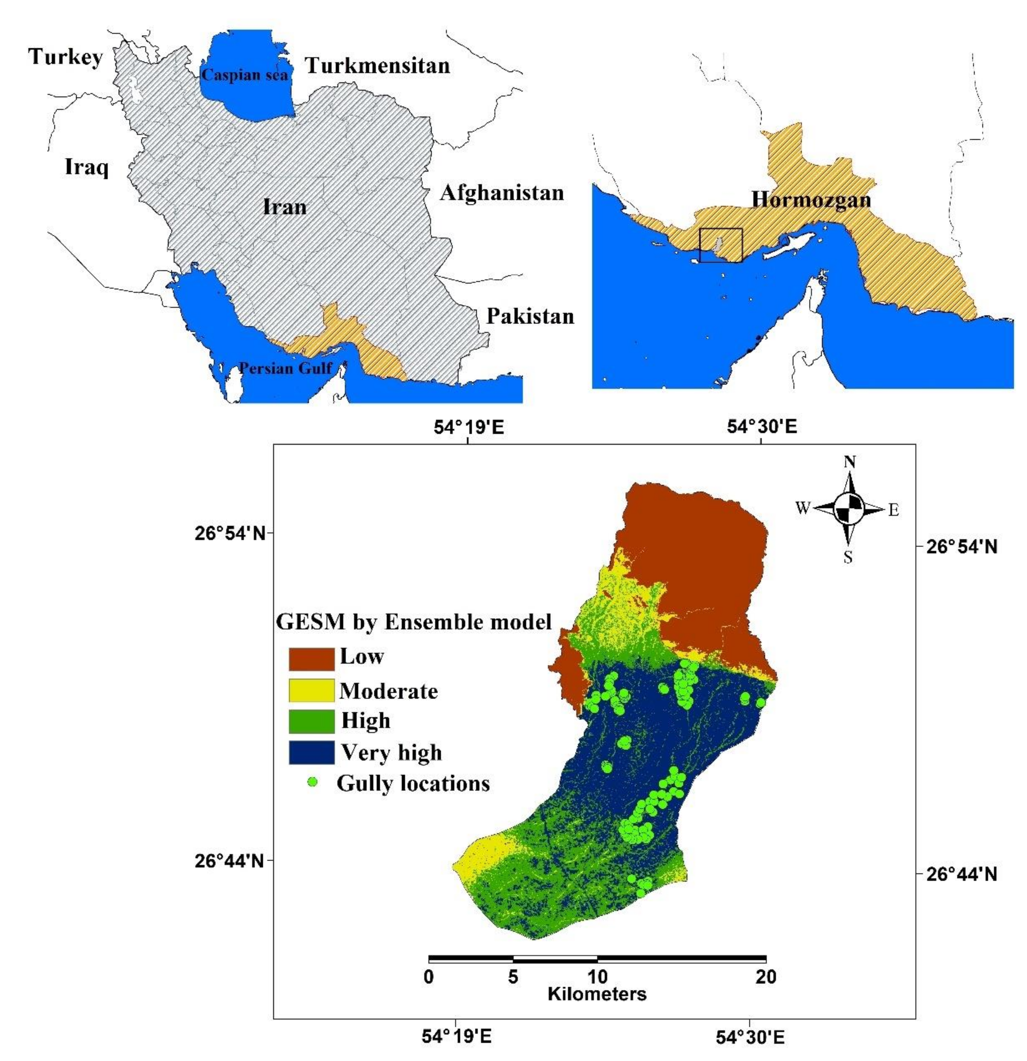
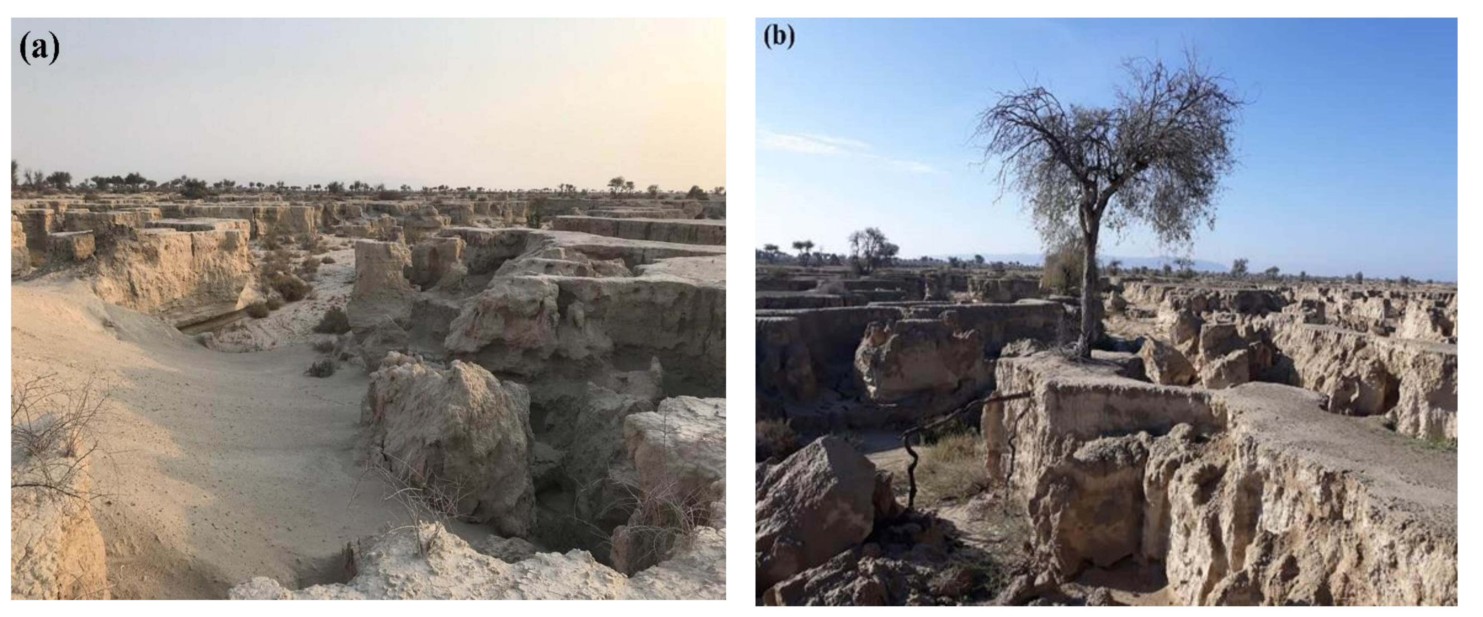
2.1. Study Area

The Kondoran watershed (KW) is located along 54°19′ to 54°30′ E longitude and 26°40′ to 26°56′ N latitude in Hormozgan province, south of Iran. Its area covers 258.86 km2 of the region, varying by 3 m to 1406 m above sea level [28]. The annual precipitation average in the study region is about 83.62 mm and the climate is hot and humid [29]. In the study area, there are several land use types including bare rock, barren lands, poor rangeland, residential lands, salt land and shrublands. The study region with an estimated population of 1628 people includes four rural regions of Armak (971 people), Kondoran (485 people), Glango (34 people) and Lavaran (138 people) [30]. Runoff and gully erosion are the main issues of the region. The soil of the region is erosion-sensitive and mostly is loamy and silty.
Soil sensitivity, heavy rains, land-use change, vegetation degradation and human interventions have caused deep gullies with depths of 1–10 m. The KW gullies contain the widest area of soil erosion in the south of Iran, which significantly has been spread toward infrastructure and settlements and has caused significant damage to roads, electrical installations, buildings, fertile lands of rural regions, and other infrastructure, and which is increasing every year. Figure 1 displays the gullies’ locations in the study region in Hormozgan province, Iran.

2.2. Data Set

The present study applied data of 140 gullies in the Kondoran watershed, collected through a field study using a GPS (Global Positioning System). Furthermore, the information of 100 gully absence places was gathered. Of these, 70% of data were randomly selected for training the learning models, and the rest (30%) were used to test and validate the fitted models [31]. Figure 2a,b shows examples of gully erosion within the study region.

2.3. Predictor Variables of Gully Erosion Susceptibility

Gullies are created under various conditions. Therefore, different variables influence gully formation and development. Selecting appropriate variables is one of the critical and effective issues in modeling gully erosion susceptibility. Various researchers have considered different variables as influence factors on gully erosion. Previous studies have considered 11 factors for gully erosion susceptibility modeling [32,33].
Figure 3 presents the methodological diagram of the present study. Using the Boruta algorithm, the most critical variables were selected for modeling gully erosion susceptibility. The evidential belief function (EBF) algorithm was applied to describe the correlation among predictor variables and gully erosion status. The gully susceptibility map in the Kondoran watershed of Hormozgan was generated by applying the multiple diagnostic analysis (MDA), support vector machine (SVM), and random forest (RF) algorithms. The models were applied to the occurrence and non-occurrence points. The AUC (area- under-the-curve) and ROC (receiver operating characteristics) have been used to assess model performance. The ensemble model was used to combine these models and produce the ensemble gully susceptibility map of the region.

2.3.1. Slope Angle

Slope angle is an essential factor that affects gully erosion. Gully erosion occurs when macropores become larger by infiltration of water into the soil [34]. The larger macropores result in a greater risk of soil collapse and gully erosion. Gentle slopes have a higher penetration rate than steeper slopes. Thus, gentle slopes are more prone to gully erosion. In this study, the slope angle map (degree) was obtained based on the digital elevation model (DEM) (Figure 4a).

2.3.2. Slope Aspect

The slope aspect is another factor that influences solar radiation reaching the ground, soil moisture, and vegetation cover [35]. Thus, it is considered an effective factor in mapping gully erosion susceptibility. The study region’s slope aspect map was generated using DEM 30 m and classified into nine classes (Figure 4b).

2.3.3. Elevation

Elevation affects the microclimate and vegetation cover. This factor affects the runoff production process as one of the main stimuli of gully erosion. Therefore, this study considered elevation as one predictor for gully erosion susceptibility modeling [36]. In the present study, a DEM of 30 m was used, extracted from a topographic map on a scale of 1:50,000 (Figure 4c).

2.3.4. Soil Texture

Soil texture and soil erodibility significantly affect gully erosions [37]. The study region’s soil texture map was provided at a 1:50,000 scale using the database of the Agricultural Research Center of Hormozgan Province [38] In this study, the soil texture is classified into four classes of loamy skeletal, coarse loamy, fine silty and fine loamy (Figure 4d).

2.3.5. Length-Slope Factor

The length-slope factor determines the influence of topography on erosion; therefore, it is considered one of the critical factors in predicting gully erosion status [39]. This factor is computed as below:
L S = F A G C e l l s i z e 22.13 0.6 × Sin ( s l o p e g r i d ) * 0.01745 0.0896 1.3
in which the FAG is the flow accumulation grid and 0.01745 is a coefficient that converts the radian to degree measure. The LS index was obtained using SAGA-GIS 7.3.6 software based on 30 m DEM (Figure 4e).

2.3.6. Plan Curvature

Plan curvature is defined as the curvature of contour lines in the horizontal plane [40]. This factor affects converging and diverging surface flow, flow rate, and soil erosion. Thus, plan curvature can be applied as an important predictor of gully erosion. The plan curvature map was generated using DEM in an ArcGIS 10.7 environment. The plan curvature map of the study area was categorized into three classes, including concave, convex and flat categories (Figure 4f). The positive and negative values of plan curvature indicate the convexity and concavity of curvature slope, and the values close to zero determine that the surface is flat [1].

2.3.7. Topographic Wetness Index

The topographic wetness index (TWI) is obtained by combining the upstream catchment area and slope, and is commonly used to quantify the topography’s influence on hydrological processes. It also determines the effect of topography on the level of saturation surface to produce runoff [41]. TWI calculates the probability of flow accumulation in soil due to the upstream catchment area and slope [42]. Thus, TWI was applied as a topographical variable for modeling gully erosion. The TW index is obtained using the following equation:
T W I = ln A s tan b
where As is the specific area of the upstream watershed (m2/m) and b is the slope angle in degree scale. In this study, the TWI was generated in SAGA-GIS software based on the 30 m DEM (Figure 4g).

2.3.8. Land Use

Land use is another factor that affects gully erosion and land degradation [13]. The land use map of the study region was provided at a 1:50,000 scale from the Agricultural Research Center of the Hormozgan Province [43]. According to Figure 4h, barren land (without vegetation), poor rangeland, bare rock, salt land, residential lands and shrublands are the main land use types of the study area. The map of the predictor variables was generated in raster format and then classified using the existing function GIS software. Table 1 indicates information on predictor variables that affect gully erosion susceptibility.

2.3.9. Lithology

The lithology factor has an important role in the gully erosion phenomenon since it depends on lithological properties and weathering of materials at the ground surface [1]. In this study, the lithological map of the study region at a 1:50,000 scale was provided from the Geological Survey of Iran [38].

2.3.10. Drainage Density

Drainage density is defined as the entire length of the channel per unit of watershed area (km/km2) [44]. Regions with higher drainage density contain lower infiltration and higher runoff. Higher drainage density facilitates the evacuation of sediments from upstream areas in watersheds, causing expanding gully erosion. Thus, drainage density can be considered a predictor variable of gully erosion hazard [36]. The study area’s drainage map was created using the line density function in an ArcGIS 10.7 environment (Figure 4j).

2.3.11. Distance to River

Distance to the river is the most important factor that affects the gully erosion process. The drainage network affects the stability and slope saturation degree, and consequently, the soil erosion process [45]. Common surface materials near the rivers contain higher moisture, which results in an acceleration of the processes of shedding, separation and soil transfer. Soil saturation depends on proximity to the stream and therefore, areas closer to streams are more susceptible to gully erosion [32]. The distance to the stream map of the study region was provided using the Euclidean distance method in ArcGIS 10.7 software. Finally, the map was classified into five categories of less than 276.5 m, 276.5 to 611.8 m, 611.8 to 1055.13 m, 1055.13 to 1806.48 m, and 1806.48 to 3118.41 m, based on the natural break approach (Figure 4k). The map of the predictor variables was generated in raster format and then classified using existing functions in GIS software. Table 1 indicates the information of predictor variables that affect gully erosion susceptibility.

2.4. Collinearity between Independent Variables

Existing collinearity between variables reduces the model’s accuracy and performance [33]. The tolerance coefficient and variance inflation factor (VIF) are two important indices for investigating dependency between variables [46]. Variables often have collinearity problems when the tolerance coefficient or VIF between them are respectively less than 0.1 or greater than 5 [7].

2.5. Boruta Variable Selection Algorithm

Feature selection is an important step in classification and regression modeling. Feature selection algorithms are used to remove the unimportant predictors to improve the model accuracy [47,48]. The Boruta algorithm is a feature selection algorithm that is placed under the RF classification method [49]. It uses shadow features which are copies of original features. The shadow features are randomly assigned to objects; therefore, decision trees are generated based on the shadow features.
The importance of an attribute is measured by the loss of accuracy of the classification model caused by attributes that are randomly assigned to objects. Then, the mean and the standard deviation of the accuracy loss are calculated, and the Z-scores are obtained by dividing the mean and its standard deviation. In the Boruta algorithm, the Z-score is considered as the measure of importance. Therefore, the set of the importance of shadow attributes is used as a reference for detecting the importance of original attributes. Then, the importance of original features is compared with the highest importance of shadow features [27]. The Boruta algorithm has the following steps:
(1)
The information system is extended by generating the shadow attributes (at least five for each attribute).
(2)
The random forest algorithms are run on each copy of the new dataset and the Z-scores are computed.
(3)
The maximum Z-score (MZS) of shadow attributes is computed.
(4)
The importance of each attribute is compared with the MZS.
(5)
The attributes with importance significantly lower than MZS are removed (considered as unimportant), and those with importance significantly higher than MZS are considered as important.
(6)
All shadow attributes are removed and the procedure is repeated until the importance is assigned to all attributes.
The Boruta algorithm has advantages in comparison with other feature selection algorithms [27]. First, this algorithm follows an all-relevant variable selection approach in which it considers all features that are related to the output variable; whereas, most of the other variable selection algorithms follow a minimum optimum approach where they depend on a small subset of features which causes a minimum error on a selected classifier. Second, it considers multi-variable relationships and also can investigate interactions between variables. In this study, the Boruta package in R software was used to determine the importance of gully erosion susceptibility factors.

2.6. Investigating the Relationship between Gully Erosion and Conditioning Factors

This study applies the evidential belief function (EBF) algorithm to describe the correlation among predictor variables and gully erosion status. The evidential belief function (EBF) is a robust approach for obtaining reliable models through incorporating various factors to reduce uncertainty [50]. The statistical EBF model is computed based on Dempster-Shafer theory to combine the representations of several independent variables to achieve a combined measure of belief.
The degree of uncertainty (Unc), degree of disbelief (Dis), degree of belief (Bel), and degree of plausibility (Pls) are the main parameters of the EBF approach, and each describes particular information of a dataset [51]. The Bel and Pls are respectively defined as the lower and upper bound of probabilities, and the uncertainty degree (Unc) is described as the difference between Bel and Pls, which shows the ignorance or doubt that the evidence supports a hypothesis. Additionally, Dis is a degree of disbelief in evidence concerning the hypothesis, and the Dis value is obtained using (1-Pls) or (1-Unc-Bel) equations.

2.7. Modeling Gully Erosion Susceptibility

2.7.1. Support Vector Machine

The support vector machine (SVM) is a supervised learning approach that is used for classification or regression modeling. This method is defined based on statistical learning theory and uses the structural risk minimization (SRM) method to obtain an optimized solution [52]. The SVM applies linear or non-linear (polynomial or radial) kernels to learn a classification model. This study applied the radial basis (RBF) kernel due to the high performance of this function. In this study, the SVM method was run using R software 3.5.3 and the SDM (Species Distribution Modelling) package [53].

2.7.2. Random Forest Model

Random forest (RF) is a classification approach that is obtained based on the improvement of bagging (bootstrap aggregation) trees [54]. The bagging tree is a decision tree that is built on bootstrap samples [55]. The main difference between random forest and bagging is the number of predictors in each bootstrapping step. On the other hand, for p predictors, the bagging trees use m = p , while the random forest splits m p predictors in each bootstrapping tree. Finally, the RF model is defined as the average of bootstrapping trees. The RF procedure is used to reduce the variance of the statistical learning method. Robustness to outliers, limiting overfitting and errors are further advantages of the RF approach [56].

2.7.3. Multiple Discriminant Analysis

Multiple discriminant analysis is a classification approach that is used to predict categorical responses. This model, also known as the Fisher discriminant analysis, is defined based on Bayes’ theorem. The MDA attempts to estimate the conditional probability and the predictors are assumed to follow a multivariate normal distribution. The linear (LDA) and quadratic (QDA) discriminant analysis are special cases of MDA used for binary responses when respectively, a linear or non-linear boundary between classes is assumed. The normality assumption of the predictor variables is a limitation of using the MDA method. For the normal case, the conditional probability leads to the linear combination for which the coefficients should be estimated [57].

2.7.4. Ensemble Model

The ensemble model (EM) is a combination of several learning models and is commonly used to improve classification algorithms by decreasing variance and bias or improving prediction accuracy [58]. Incorporating the single models’ predictions is done using weighted and unweighted averaging. In this study, the ensemble model was assembled using weighted averaging based on AUC statistics Equation (3):
E M = i = 1 n ( A U C i * M ^ i ) i = 1 n A U C i
where EM is the ensemble model, and AUCi is the AUC value of the ith single model (Mi).
In the present study, the SVM, RF, MDA and ensemble methods have been run using R software 3.5.3 and the SDM (Species Distribution Modelling) package [53]. The probability maps were provided based on all models and were classified using the natural break method in ArcGIS 10.7. The classification map obtained from the EM is different from the maps obtained from the other three models. This is because the EM is the weighted average of SVM, RF and MDA models using the AUC weighting and the unclassified maps of every single model are merged to create an ensemble model. To merge the unclassified output map of single models, the weighted average is used.

2.7.5. Evaluation Model Performance

This study applied AUC (area under the receiver operating characteristic curve) and True Skill Statistics (TSS) to evaluate model performance. The AUC statistics describe the area under the receiving operator characteristics curve (ROC) and are used as a measure of classification accuracy. The greater AUC indicates a better classification result [58]. Each observation belongs to a positive (gully existence) or negative (non-existence) category in gully classification. The AUC determines the classification accuracy based on the ROC. The number of positive and negative pixels correctly classified is called true positive (TP) or true negative (TN). In contrast, it can be defined as the false positive (FP) and false-negative (FN) for wrongly classified pixels [59]. In the ROC curve, the X-axes represent the specificity and Y-axes indicate the sensitivity and are defined as below:
S e n s i t i v i t y = T P T P + F N
S p e c i f i c i t y = T N F P + T N
The AUC varies between 0 and 1, such that a value close to 0 indicates that the learning model is not able to classify the observations, while an AUC close to 1 shows that the observations are classified very well [60]. In addition, an AUC less than 0.6, between 0.6 to 0.8, and greater than 0.8, describes low, moderate and high classification accuracy, respectively [33].
The true skill statistic (TSS), also known as Hanssen–Kuipers discriminant, is another common measure for evaluating classification accuracy [61]. TSS statistics explain the ratio of true predictions (true positive and true negative) [62]. TSS value changes between −1 to +1, where +1 determines high classification accuracy and values below zero show a performance no better than random [62]. The TSS is computed as TSS = Sensitivity + Specificity−1.

3. Results

3.1. Multi-Collinearity Test

Multi-collinearity is a serious problem in regression and classification, and refers to a situation in which two or more predictor variables are linearly correlated. In this study, we applied variance inflation factor (VIF) and tolerance (TOL) criteria to explore collinearity between explanatory variables. According to these criteria, a TOL less than 0.1 and a VIF above 10 indicate that there exists a collinearity problem among predictor variables. Table 2 provided VIF and TOL values between gully erosion predictors. As shown, there exists no collinearity between predictor variables.

3.2. Gully Erosion Susceptibility Maps (GESM)

The maps of gully erosion susceptibility were generated using effective parameters based on the SVM, RF and MAD models. Next, a new map was provided using the ensemble model, which was defined based on the RF, MAD and SVM models. The maps were classified into low, moderate, high, and very high susceptibility classes using the natural break classification method (Figure 5). The results revealed that most parts of the study region are allocated in the very high susceptibility category. Further analysis of Table 3 indicated that the MDA model allocated the lowest part (429 km2, 1.67%) and the highest part (169.93 km2, 66.03%) of the study regions respectively assigned to the moderate and very high susceptibility, while according to the SVM model, the lowest part (31.06 km2, 12.07%) and the highest part (121.52 km2, 47.22%) of the study regions belong to the low and very high susceptibility classes. In this regard, based on the RF and ensemble models, the low susceptibility areas respectively covered 73.37 km2 (28.51%) and 74.34 km2 (28.88%) of the study regions, while very high susceptibility areas respectively covered 84.07 km2 (32.67%) and 97.69 km2 (37.96%) of the study region. According to the results, in all models, the study area’s central and eastern parts belong to the very high susceptibility class and the northern parts of the region are in the low susceptibility class.

3.3. Evaluation of GESMs Performance

The performance of the fitted models for the gully erosion susceptibility maps was evaluated using area-under-the-curve (AUC) and true skill statistics (TSS). The results are reported in Table 4 and Figure 6. All models present high values in both AUC and TSS. The ensemble model had the highest values in both criteria. Thus, the accuracy among the fitted models in predicting gully erosion susceptibility is high.

3.4. Computing Variable Importance Using Boruta Algorithm

Results and outputs of the Boruta algorithm (Table 5) indicate that distance to the stream (33.5), land use (17.41), elevation (12.18), and lithology (7.34) are the most important gully erosion factors, followed by soil type, drainage density, LS factor, and slope angle. In addition, the plan curvature, TWI, and slope aspects have the least rank among the predictor variables and should be ignored from the modeling process.

3.5. Evaluating the Relationship among Conditioning Factors and Gully Erosion Using the Evidential Belief Function (EBF) Model

The relationship between gully erosion and predictor variables was investigated and results are shown in Table 6. According to the results, the highest weight of distance to streams variable (0.51) has been assigned to class 1, [0–276.5], and is regarded as the most effective factor on gully erosion occurrence in the study area. For this factor, higher distances (>1055.3 m) have zero weight in Bel measure. In this regard, the class [1.8–3.69] km/km2 of drainage density variable had the highest Bel (0.45) weight and is considered as the area with a high probability of gully occurrence. The highest correlation (Bel = 0.44) of gully erosion with TWI variable belongs to the [12–22.3] class, which denotes a positive correlation between these two variables.
In the case of elevation factor, the complete correlation (Bel = 1) between gully erosion and [3–125] m category denoted that the gully erosion generally occurs in lowlands and there is a low probability for the gully erosion occurrence in higher elevation lands. Additionally, the results of the relationship between gully erosion and slope length factor indicated that the highest Bel value (0.88) was observed at the [0–2.5] class, signifying that commonly, the gully erosion in the region occurs with low slope length (<5.91). In the case of slope degree, the highest Bel value was observed between gully erosion and the [<10°] classes. Further, the slope aspect results determined that most of the gullies have been formed (Bel = 0.25) in the north-east directions in the study area.
In the case of the lithology variable, the highest correlation (Bel = 0.71) was obtained between gully erosion and Qfp, followed respectively by Qal and Qaf classes. In other lithological units, the Bel value was zero. The plan curvature is another predictor variable that defines the curvature of a contour line in the horizontal plane and determines a region’s position [45,63]. As the result indicated, the [−0.1 −0.1] curvature class had the highest impact (Bel = 1) on gully erosion occurrence, compared to the other curvature classes.
Concerning the land-use variable, most gully erosions have occurred in the barren lands (0.71), followed by shrublands (0.29). Finally, the soil type analysis indicated that the highest correlation (Bel = 0.94) was observed between gully erosion and the fine silty soil texture category, followed by the coarse loamy class (Bel = 0.06).

4. Discussion

Gully erosion constitutes a serious problem for land degradation in a wide range of environments. The Kondoran watershed is one of the most susceptible regions to gullying in the Hormozgan province due to environmental factors and human interventions. Indeed, this study provides an understandable platform to inform decision-makers about the current situation of this study area. To this end, we evaluated gully erosion susceptibility in the study area based on multiple diagnostic analysis (MDA), support vector machine, and random forest (RF) algorithms, and also a combination of these models, namely the ensemble model.
Each of the models contains specific weaknesses in modeling gully susceptibility mapping, which can be resolved using the ensemble modeling method. The ensemble method is a procedure that combines a specific number of learning models in such a way that its predicted response is the weighted average of the predicted response obtained from the incorporated models [26]. The evaluation of the performance of models showed that the ensemble model had the highest accuracy in predicting gully erosion susceptibility. These results are consistent with the findings of Pourghasemi et al. [64] in using the ensemble model for predicting gully erosion susceptibility.
The outputs of fitted models were spatially different because it depends on the different structures of the models, and also the importance of input variables to each model. For instance, the MDA model is highly correlated with altitude, the SVM model has the highest correlation with LS factor, while the RF and the ensemble models showed the highest correlation with the distance to the stream predictors. The Boruta feature selection algorithm was applied to determine the most important gully erosion factors. Results and outputs of the Boruta algorithm indicated that distance to the stream was the most influential factor on gully erosion susceptibility. This result corroborates the findings of Conoscenti et al. [45], and Rahmati et al. [61].
The relationship between gully erosion and predictor variables was investigated using the EBF model. The results showed that the highest weight of distance to streams variable had been assigned to the regions with the nearest distance to streams. Therefore, most gullies in study regions have been formed close to the streams because the soils near streams are water-saturated, and as a result, the disintegration and collapse of soil particles intensifies; subsequently, gully erosion susceptibility increases [64]. The regions with the most drainage density had a high probability of gully occurrence due to lower infiltration and more runoff events [31]. The highest correlation of gully erosion with the TWI variable belongs to the regions with the higher topographic wetness. Generally, the higher topographic wetness results in a higher probability of occurrence of gully erosion, corroborating with Pourghasemi et al. [64] and Hembram et al. [65].
The study of elevation factor indicated that gully erosion generally occurs in lowlands and there is a low probability for the gully erosion occurrence in higher elevation lands. The probability of washing and disintegrating the soil particles increases in lowland regions because the runoff accumulation is higher than in elevated regions. As a result, the gully erosion hazard increases in lowlands, in line with the findings of Dickson et al. [66] and Amiri et al. [7]. According to the results, the regions with lower slope angles and slope length are more prone to gully erosion than the regions with higher slope angles and slope length, and this is similar to the findings of Azareh et al. [32]. When the slope increases, the water velocity increases; subsequently, the soil erosion rate increases. However, gully erosion generally forms on low slopes and flat areas. In other words, to form a gully erosion, water flow should accumulate at a point and create a hole; a phenomena which commonly happens to low slopes.
Investigating the lithology variable indicated that the highest gully erosion has occurred in Quaternary floodplain deposits (Qfp). These sediments contain fine-grained floodplain deposits, silt, and fine-grained sand and clay. Therefore, these regions are the most susceptible to gully erosion. In the case of the land-use variable, most gully erosions have occurred in the barren lands that, due to the lack of vegetation, are more susceptible to gully erosion. This is consistent with the finding of Fernández-Raga et al. [62]. Soil type analysis showed that most gully erosions have occurred in the fine silty category, followed by the coarse loamy class. These soils are more susceptible to erosion because their particles are easily separated and transferred after moisture absorption, and thereby cause the gully erosion phenomenon [67,68].
Raising the level of public awareness about this phenomenon, not interfering and misappropriating in nature, preventing the destruction of natural resources, preventing land-use change and runoff management in watersheds by implementing watershed management projects, especially rainwater harvesting systems and vegetation restoration, can be considered as some of the most important preventive measures in controlling gully erosion and land degradation in the Hormozgan province [69].
The study of gully erosion susceptibility maps indicated that, in all models, the central and eastern parts of the studied region belong to a very high sensitivity class, while the northern part of the region is located in the low sensitivity class. Most of the gullies are located in lowlands, near the streams, in silty soils, in barren lands and shrublands, and in proximity to the rural settlements. In the past few years, the gully erosion was expanded toward the Kondoran and Armak villages lands in the middle part of the study region. Therefore, experts and planners should prioritize the management of these lands to reduce damages caused by gully erosion. Distance to streams and elevation cannot change; meanwhile, restoration and development of the degraded land might change the land use and decrease the susceptibility to gully erosion [70,71]. Additionally, sustainable soil management could be achieved by afforestation of the barren lands and regenerative agriculture techniques in areas most susceptible to gully erosion [72,73].

5. Conclusions

In recent years, gully erosion has caused losses of a large volumes of soil in the Kondoran watershed in Hormozgan province, Iran. Therefore, accurate prediction of gully erosion susceptibility is a fundamental issue to protect the soil and reduce the erosion rate. This study applied four classification models, including random forest (RF), support vector machine (SVM), multivariate discriminant analysis (MDA), and the ensemble model (as the combination of the three previous models) to provide gully erosion maps of the study region. The accuracy of gully erosion susceptibility maps was evaluated using the area under ROC curve (AUC) and TSS metrics. Results and outputs indicated that the ensemble method (AUC = 98.2%, TSS = 0.93) has better performance than the RF (AUC = 97.1%, TSS = 0.91), SVM (AUC = 93.2%, TSS = 0.84) and MDA (AUC = 91.4%, TSS = 0.82) models.
The Boruta feature selection algorithm was used to determine the most important factors in gully erosion susceptibility mapping. It was found that gully occurrence in the study area was mainly influenced by topological factors (elevation, and distance from streams), anthropogenic factors (land use and proximity to rural settlements), and geological factors (lithology and soil texture). Further, the results of the Boruta algorithm denoted that the plan curvature, TWI, and slope aspect could be ignored from the modeling process. The results indicated that the central, eastern, and southern parts of the study area are more susceptible to gully erosion. Models and predictors applied in this study can be used in similar areas. Regenerative agriculture techniques and afforestation of these lands should be prioritized to reduce land degradation in the present and future.

Author Contributions

Conceptualization, H.A. and O.B.; methodology, H.A. and E.R.-S.; software, E.R.-S.; validation, E.R.-S.; formal analysis, H.A.; investigation, H.A.; resources, H.Z.; data curation, H.Z.; writing—original draft preparation, H.A.; writing—review and editing, T.P.; supervision, O.B. and T.P.; funding acquisition, T.P. All authors have read and agreed to the published version of the manuscript.

Funding

The Fundação para a Ciência e Tecnologia, grant number PTDC/GES-URB/31928/2017.

Institutional Review Board Statement

Not applicable.

Informed Consent Statement

Not applicable.

Data Availability Statement

Data will be available uppon request.

Acknowledgments

The research center CINTURS and the Fundação para a Ciência e Tecnologia supported this paper under grant PTDC/GES-URB/31928/2017.

Conflicts of Interest

The authors declare no conflict of interest.

Appendix A

Table A1. The abbreviations included in the text are reported alphabetically.
AGNPS Agricultural Non-point Source AGNPS is a computer-simulation model that simulates the behavior of runoff, sediment, and nutrient transport from watersheds that have agriculture as their prime use. The model operates on a cell basis and is a distributed parameter, event-based model.
AUC of ROC Area-under-the-curve of Receiver Operating CharacteristicsThe AUC statistics describe the area under the ROC curve and are used as a measure of classification accuracy. The greater AUC indicates a better classification result.
BelBeliefBelief is one of the functions that is used in EBF model. It is the pessimistic measures of the spatial relationship of response variable, i.e., Bel indicates the lower probabilities of evidence that supports a hypothesis.
DEMDigital Elevation ModelA digital elevation model (DEM) is a representation of the bare ground (bare earth) topographic surface of the Earth excluding trees, mountains, buildings, and any other surface objects.
DisDisbeliefDisbelief is one of the functions that is used in EBF model. It is a degree of disbelief in evidence for the hypothesis and the Dis value is obtained from 1–Pls or 1-Unc–Bel.
EBF Evidential Belief FunctionThe evidential belief function (EBF) algorithm describes the correlation among predictor variables and response variable. The statistical EBF model is computed based on Dempster-Shafer’s theory to combine the representations of several independent variables to achieve a combined measure of belief.
GISGeographic Information System A geographic information system (GIS) is a conceptualized framework that provides the ability to capture and analyze spatial and geographic data.
GLMGeneralized Linear ModelGLM is the extension of the classic linear regression model. Contrasted with the normal linear model, the response variables of GLM are not confined to normal distribution, and these response variables can also obey binomial or Poisson distributions. In addition, the link function is introduced into GLM to establish the relationship between the expectation of the response variable and the linear combination of explanatory variables.
GPS Global Positioning SystemGPS (Global Positioning System) is a radio wave receiver used to provide coordinates that give the exact position of an element in a certain space.
LiDARLight Detection and RangingLiDAR is a method for determining ranges (variable distance) by targeting an object with a laser and measuring the time for the reflected light to return to the receiver.
LISEM Limburg Soil Erosion ModelThe Limburg soil erosion model (LISEM) is a physically-based hydrological and soil erosion model which can be used for planning and conservation purposes.
MaxEnt Maximum EntropyMaxEnt is a data mining method to predict the occurrence of one event based on maximum entropy that approximates the probability distribution of presence data based on environmental limitations.
MDAMultiple Diagnostic AnalysisMultiple discriminant analysis is a classification approach that is used to predict categorical responses. This model, also known as the Fisher discriminant analysis, is defined based on Bayes’ theorem. The MDA attempts to estimate the conditional probability and the predictors are assumed to follow a multivariate normal distribution.
PlsPlausibilityPlausibility is one of the functions that is used in EBF model. It is the optimistic measures of the spatial relationship of response variable, i.e., Pls indicates the upper probabilities of evidence that supports a hypothesis.
RFRandom ForestRandom forest (RF) is a classification approach that is obtained based on the improvement of bagging (bootstrap aggregation) trees.
RUSLERevised Universal Soil Loss EquationRUSLE is an easily and widely used model that estimates rates of soil erosion caused by rainfall and associated overland flow.
SAR Synthetic Aperture RadarSynthetic aperture radar (SAR) is a form of radar that is used to create two-dimensional images or three-dimensional reconstructions of objects, such as landscapes. SAR uses the motion of the radar antenna over a target region to provide finer spatial resolution than conventional stationary beam-scanning radars.
SVMSupport Vector MachineThe support vector machine (SVM) is a supervised learning approach that is used for classification or regression modeling. This method is defined based on statistical learning theory and uses the structural risk minimization (SRM) method to obtain an optimized solution.
TOLToleranceTolerance is relevant and frequently used quantities that may be consulted to examine individual predictors for potentially strong contributions to (near) multicollinearity. This index reflects estimates of the degree of interrelationship of an independent variable with other explanatory variables in a regression model. The TOL less than 0.1 indicates that there exists a collinearity problem among predictor variables.
TSSTrue Skill StatisticThe true skill statistic (TSS) is known as Hanssen–Kuipers discriminant, and is commonly measure for evaluating classification accuracy. The true skill statistics is defined based on the components of the standard confusion matrix representing matches and mismatches between observations and predictions.
TWITopographic Wetness IndexThe topographic wetness index (TWI) is a physically-based index of the effect of local topography on runoff flow direction and accumulation. The index is a function of both the slope and the upstream contributing area. The computation of TWI is performed using both geographic information systems (GIS) and Python, a programing software used to enhance computing capabilities. The indices help identify rainfall runoff patterns, areas of potential increased soil moisture, and ponding areas.
Unc UncertaintyUnc value is one of the functions that is used in EBF model. It is the difference between the Pls and Bel function, which shows the ignorance or doubt that the evidence supports a hypothesis.
VIF Variance Inflation FactorVariance inflation factor measures how much the behavior (variance) of an independent variable is influenced, or inflated, by its interaction/correlation with the other independent variables. Variance inflation factors allow a quick measure of how much a variable is contributing to the standard error in the regression. VIF is the reciprocal of Tolerance. The VIF above 10 indicates that there exists a collinearity problem among predictor variables.

References

  1. Liu, G.; Zheng, F.; Wilson, G.V.; Xu, X.; Liu, C. Three decades of ephemeral gully erosion studies. Soil Tillage Res. 2021, 212, 105046. [Google Scholar] [CrossRef]
  2. Conforti, M.; Aucelli, P.P.C.; Robustelli, G.; Scarciglia, F. Geomorphology and GIS analysis for mapping gully erosion susceptibility in the Turbolo stream catchment (Northern Calabria, Italy). Nat. Hazards 2011, 56, 881–898. [Google Scholar] [CrossRef]
  3. Mokarram, M.; Zarei, A.R. Determining prone areas to gully erosion and the impact of land use change on it by using multiple-criteria decision-making algorithm in arid and semi-arid regions. Geoderma 2021, 403, 115379. [Google Scholar] [CrossRef]
  4. Conoscenti, C.; Rotigliano, E. Predicting gully occurrence at watershed scale: Comparing topographic indices and multivariate statistical models. Geomorphology 2020, 359, 107123. [Google Scholar] [CrossRef]
  5. Gómez-Gutiérrez, A.; Conoscenti, C.; Angileri, S.E.; Rotigliano, E.; Schnabel, S. Using topographical attributes to evaluate gully erosion proneness (susceptibility) in two mediterranean basins: Advantages and limitations. Nat. Hazards 2015, 79, 291–314. [Google Scholar] [CrossRef]
  6. Amiri, M.; Pourghasemi, H.R.; Ghanbarian, G.A.; Afzali, S.F. Assessment of the importance of gully erosion effective factors using Boruta algorithm and its spatial modeling and mapping using three machine learning algorithms. Geoderma 2019, 340, 55–69. [Google Scholar] [CrossRef]
  7. Lei, P.; Shrestha, R.; Zhu, B.; Han, S.; Yang, H.; Tan, S.; Ni, J.; Xie, D. A Bibliometric Analysis on Nonpoint Source Pollution: Current Status, Development, and Future. Int. J. Environ. Res. Public Healthy 2021, 18, 7723. [Google Scholar] [CrossRef] [PubMed]
  8. Hessel, R. Effects of grid cell size and time step length on simulation results of the Limburg soil erosion model (LISEM). Hydrol. Process. 2005, 19, 3037–3049. [Google Scholar] [CrossRef]
  9. Ferreira, V.; Panagopoulos, T. Seasonality of Soil Erosion Under Mediterranean Conditions at the Alqueva Dam Watershed. Environ. Manag. 2014, 54, 67–83. [Google Scholar] [CrossRef]
  10. Ferreira, V.; Samora-Arvela, A.; Panagopoulos, T. Soil erosion vulnerability under scenarios of climate land-use changes after the development of a large reservoir in a semi-arid area. J. Environ. Plan. Manag. 2016, 59, 1238–1256. [Google Scholar] [CrossRef]
  11. Zare, M.; Panagopoulos, T.; Loures, L. Simulating the impacts of future land use change on soil erosion in the Kasilian watershed, Iran. Land Use Policy 2017, 67, 558–572. [Google Scholar] [CrossRef]
  12. Fiorucci, F.; Ardizzone, F.; Rossi, M.; Torri, D. The Use of Stereoscopic Satellite Images to Map Rills and Ephemeral Gullies. Remote Sens. 2015, 7, 14151–14178. [Google Scholar] [CrossRef] [Green Version]
  13. Bingner, R.L.; Wells, R.R.; Momm, H.G.; Rigby, J.R.; Theurer, F.D. Ephemeral gully channel width and erosion simulation technology. Nat. Hazards 2015, 80, 1949–1966. [Google Scholar] [CrossRef]
  14. Rahman, R.; Shi, Z.; Chongfa, C. Soil erosion hazard evaluation—An integrated use of remote sensing, GIS and statistical approaches with biophysical parameters towards management strategies. Ecol. Model. 2009, 220, 1724–1734. [Google Scholar] [CrossRef]
  15. Soleimanpour, S.M.; Pourghasemi, H.R.; Zare, M. A comparative assessment of gully erosion spatial predictive modeling using statistical and machine learning models. Catena 2021, 207, 105679. [Google Scholar] [CrossRef]
  16. Hembram, T.K.; Paul, G.C.; Saha, S. Spatial prediction of susceptibility to gully erosion in Jainti River basin, Eastern India: A comparison of information value and logistic regression models. Model. Earth Syst. Environ. 2018, 5, 689–708. [Google Scholar] [CrossRef]
  17. Arabameri, A.; Pradhan, B.; Rezaei, K. Spatial prediction of gully erosion using ALOS PALSAR data and ensemble bivariate and data mining models. Geosci. J. 2019, 23, 669–686. [Google Scholar] [CrossRef]
  18. Pourghasemi, H.R.; Sadhasivam, N.; Kariminejad, N.; Collins, A. Gully erosion spatial modelling: Role of machine learning algorithms in selection of the best controlling factors and modelling process. Geosci. Front. 2020, 11, 2207–2219. [Google Scholar] [CrossRef]
  19. Saha, S.; Roy, J.; Arabameri, A.; Blaschke, T.; Bui, D.T. Machine Learning-Based Gully Erosion Susceptibility Mapping: A Case Study of Eastern India. Sensors 2020, 20, 1313. [Google Scholar] [CrossRef] [Green Version]
  20. Javidan, N.; Kavian, A.; Pourghasemi, H.R.; Conoscenti, C.; Jafarian, Z. Data Mining Technique (Maximum Entropy Model) for Mapping Gully Erosion Susceptibility in the Gorganrood Watershed, Iran. In Gully Erosion Studies from India and Surrounding Regions; Springer: Cham, Switzerland, 2020; pp. 427–448. [Google Scholar]
  21. Rivera, J.I.; Bonilla, C.A. Predicting soil aggregate stability using readily available soil properties and machine learning techniques. Catena 2020, 187, 104408. [Google Scholar] [CrossRef]
  22. Elith, J.; Leathwick, J.R.; Hastie, T. A working guide to boosted regression trees. J. Anim. Ecol. 2008, 77, 802–813. [Google Scholar] [CrossRef] [PubMed]
  23. Etemadi, H.; Rostamy, A.A.A.; Dehkordi, H.F. A genetic programming model for bankruptcy prediction: Empirical evidence from Iran. Expert Syst. Appl. 2009, 36, 3199–3207. [Google Scholar] [CrossRef]
  24. Gupta, L.D.; Malviya, A.K.; Singh, S. Performance Analysis of Classification Tree Learning Algorithms. Int. J. Comput. Appl. 2012, 55, 39–44. [Google Scholar] [CrossRef]
  25. Chen, W.; Lei, X.; Chakrabortty, R.; Pal, S.C.; Sahana, M.; Janizadeh, S. Evaluation of different boosting ensemble machine learning models and novel deep learning and boosting framework for head-cut gully erosion susceptibility. J. Environ. Manag. 2021, 284, 112015. [Google Scholar] [CrossRef]
  26. Arabameri, A.; Yamani, M.; Pradhan, B.; Melesse, A.; Shirani, K.; Bui, D.T. Novel ensembles of COPRAS multi-criteria decision-making with logistic regression, boosted regression tree, and random forest for spatial prediction of gully erosion susceptibility. Sci. Total. Environ. 2019, 688, 903–916. [Google Scholar] [CrossRef]
  27. Kursa, M.; Rudnicki, W. Feature Selection with theBorutaPackage. J. Stat. Softw. 2010, 36, 1–13. [Google Scholar] [CrossRef] [Green Version]
  28. Azhdari, Z.; Sardooi, E.R.; Bazrafshan, O.; Zamani, H.; Singh, V.P.; Saravi, M.M.; Ramezani, M. Impact of climate change on net primary production (NPP) in south Iran. Environ. Monit. Assess. 2020, 192, 1–16. [Google Scholar] [CrossRef]
  29. Department of Water Resource Management of Iran (DWRMI). Report of Natural Resources Management; Ministry of Energy of Iran: Tehran, Iran, 2012; 245p.
  30. Statistical Center of Iran. Available online: https://www.amar.org.ir/english/Population-and-Housing-Censuses (accessed on 20 August 2016).
  31. Cama, M.; Conoscenti, C.; Lombardo, L.; Rotigliano, E. Exploring relationships between grid cell size and accuracy for debris-flow susceptibility models: A test in the Giampilieri catchment (Sicily, Italy). Environ. Earth Sci. 2016, 75, 1–21. [Google Scholar] [CrossRef]
  32. Azareh, A.; Rahmati, O.; Rafiei-Sardooi, E.; Sankey, J.B.; Lee, S.; Shahabi, H.; Bin Ahmad, B. Modelling gully-erosion susceptibility in a semi-arid region, Iran: Investigation of applicability of certainty factor and maximum entropy models. Sci. Total Environ. 2019, 655, 684–696. [Google Scholar] [CrossRef]
  33. Arabameri, A.; Chen, W.; Loche, M.; Zhao, X.; Li, Y.; Lombardo, L.; Cerda, A.; Pradhan, B.; Bui, D.T. Comparison of machine learning models for gully erosion susceptibility mapping. Geosci. Front. 2020, 11, 1609–1620. [Google Scholar] [CrossRef]
  34. Tao, Y.; Zou, Z.; Guo, L.; He, Y.; Lin, L.; Lin, H.; Chen, J. Linking soil macropores, subsurface flow and its hydrodynamic characteristics to the development of Benggang erosion. J. Hydrol. 2020, 586, 124829. [Google Scholar] [CrossRef]
  35. Kumar, R.; Anbalagan, R. Landslide susceptibility zonation in part of Tehri reservoir region using frequency ratio, fuzzy logic and GIS. J. Earth Syst. Sci. 2015, 124, 431–448. [Google Scholar] [CrossRef]
  36. Gayen, A.; Pourghasemi, H.R.; Saha, S.; Keesstra, S.; Bai, S. Gully erosion susceptibility assessment and management of hazard-prone areas in India using different machine learning algorithms. Sci. Total Environ. 2019, 668, 124–138. [Google Scholar] [CrossRef] [PubMed]
  37. Auerswald, K.; Fiener, P.; Martin, W.; Elhaus, D. Use and misuse of the K factor equation in soil erosion modeling: An alternative equation for determining USLE nomograph soil erodibility values. Catena 2014, 118, 220–225. [Google Scholar] [CrossRef]
  38. Agricultural Research, Education and Extension Organization of Hormozgan, Bandar Abbas, Iran. Available online: http://hormozgan.areeo.ac.ir/fa-IR/hormozgan.areeo.ac/3853/page (accessed on 5 July 2019).
  39. Renard, K.G.; Foster, G.R.; Weesies, G.A.; McCool, D.K.; Yoder, D.C. Predicting Soil Erosion by Water: A Guide to Conservation Planning with the Revised Universal Soil Loss Equation (RUSLE); United States Government Printing: Washington, DC, USA, 1997; Volume 703, pp. 145–220.
  40. Wilson, J.P.; Gallant, J.C. Digital Terrain Analysis. Principles and Applications; John Wiley: New York, NY, USA, 2000. [Google Scholar]
  41. Qin, C.-Z.; Zhu, A.-X.; Pei, T.; Li, B.-L.; Scholten, T.; Behrens, T.; Zhou, C.-H. An approach to computing topographic wetness index based on maximum downslope gradient. Precis. Agric. 2011, 12, 32–43. [Google Scholar] [CrossRef]
  42. Waga, K.; Malinen, J.; Tokola, T. A Topographic Wetness Index for Forest Road Quality Assessment: An Application in the Lakeland Region of Finland. Forests 2020, 11, 1165. [Google Scholar] [CrossRef]
  43. Geological Survey of Iran [GSI]. Available online: http://www.gsi.ir/en (accessed on 25 August 2019).
  44. Glennon, A.; Groves, C. An examination of perennial stream drainage patterns within the Mammoth Cave watershed, Kentucky. J. Cave Karst Stud. 2002, 64, 82–91. [Google Scholar]
  45. Conoscenti, C.; Angileri, S.E.; Cappadonia, C.; Rotigliano, E.; Agnesi, V.; Maerker, M. Gully erosion susceptibility assessment by means of GIS-based logistic regression: A case of Sicily (Italy). Geomorphology 2014, 204, 399–411. [Google Scholar] [CrossRef] [Green Version]
  46. Greene, W.H. Econometric Analysis; Prentice Hall: Upper Saddle River, NJ, USA, 2002. [Google Scholar]
  47. Sánchez-Maroño, N.; Alonso-Betanzos, A.; Calvo-Estévez, R.M. A Wrapper Method for Feature Selection in Multiple Classes Datasets; Springer: Berlin/Heidelberg, Germany, 2009; pp. 456–463. [Google Scholar] [CrossRef]
  48. Kursa, M.B.; Jankowski, A.; Rudnicki, W. Boruta-A system for feature selection. Fundam. Inform. 2010, 101, 271–285. [Google Scholar] [CrossRef]
  49. Breiman, L. Random Forests. Mach. Learn. 2001, 45, 5–32. [Google Scholar] [CrossRef] [Green Version]
  50. Thiam, A.K. An Evidential Reasoning Approach to Land Degradation Evaluation: Dempster-Shafer Theory of Evidence. Trans. GIS 2005, 9, 507–520. [Google Scholar] [CrossRef]
  51. Althuwaynee, O.F.; Pradhan, B.; Park, H.J.; Lee, J.H. A novel ensemble bivariate statistical evidential belief function with knowledge-based analytical hierarchy process and multivariate statistical logistic regression for landslide susceptibility mapping. Catena 2014, 114, 21–36. [Google Scholar] [CrossRef]
  52. Vapnik, V.N. The Nature of Statistical Learning Theory, 2nd ed.; Springer: New York, NY, USA, 1999. [Google Scholar]
  53. Naimi, B.; Araújo, M.B. sdm: A reproducible and extensible R platform for species distribution modelling. Ecography 2016, 39, 368–375. [Google Scholar] [CrossRef] [Green Version]
  54. James, G.; Witten, D.; Hastie, T.; Tibshirani, R. An Introduction to Statistical Learning; Springer: New York, NY, USA, 2013. [Google Scholar]
  55. Liaw, A.; Wiener, M. Classification and regression by random Forest. R News 2013, 2, 18–22. [Google Scholar]
  56. Wang, Y.; Brandt, M.; Zhao, M.; Tong, X.; Xing, K.; Xue, F.; Kang, M.; Wang, L.; Jiang, Y.; Fensholt, R. Major forest increase on the Loess Plateau, China (2001–2016). Land Degrad. Dev. 2018, 29, 4080–4091. [Google Scholar] [CrossRef]
  57. Johnson, R.A.; Wichern, D.W. Applied Multivariate Statistical Analysis; Prentice Hall: Upper Saddle River, NJ, USA, 2002. [Google Scholar]
  58. Zabihi, M.; Mirchooli, F.; Motevalli, A.; Darvishan, A.K.; Pourghasemi, H.R.; Zakeri, M.A.; Sadighi, F. Spatial modelling of gully erosion in Mazandaran Province, northern Iran. Catena 2018, 161, 1–13. [Google Scholar] [CrossRef]
  59. Schumann, G.J.-P.; Vernieuwe, H.; De Baets, B.; Verhoest, N.E.C. ROC-based calibration of flood inundation models. Hydrol. Process. 2014, 28, 5495–5502. [Google Scholar] [CrossRef]
  60. Evans, R.; Horstman, C.; Conzemius, M. Accuracy and Optimization of Force Platform Gait Analysis in Labradors with Cranial Cruciate Disease Evaluated at a Walking Gait. Veter-Surg. 2005, 34, 445–449. [Google Scholar] [CrossRef]
  61. Rahmati, O.; Falah, F.; Naghibi, S.A.; Biggs, T.; Soltani, M.; Deo, R.C.; Cerdà, A.; Mohammadi, F.; Bui, D.T. Land subsidence modelling using tree-based machine learning algorithms. Sci. Total Environ. 2019, 672, 239–252. [Google Scholar] [CrossRef]
  62. Allouche, O.; Tsoar, A.; Kadmon, R. Assessing the accuracy of species distribution models: Prevalence, kappa and the true skill statistic (TSS). J. Appl. Ecol. 2006, 43, 1223–1232. [Google Scholar] [CrossRef]
  63. Choi, Y.; Park, H.-D.; Sunwoo, C. Flood and gully erosion problems at the Pasir open pit coal mine, Indonesia: A case study of the hydrology using GIS. Bull. Eng. Geol. Environment. 2008, 67, 251–258. [Google Scholar] [CrossRef]
  64. Pourghasemi, H.R.; Yousefi, S.; Kornejady, A.; Cerdà, A. Performance assessment of individual and ensemble data-mining techniques for gully erosion modeling. Sci. Total Environ. 2017, 609, 764–775. [Google Scholar] [CrossRef] [Green Version]
  65. Hembram, T.K.; Paul, G.C.; Saha, S. Modelling of gully erosion risk using new ensemble of conditional probability and index of entropy in Jainti River basin of Chotanagpur Plateau Fringe Area, India. Appl. Geomat. 2020, 12, 337–360. [Google Scholar] [CrossRef]
  66. Dickson, J.L.; Head, J.W.; Kreslavsky, M. Martian gullies in the southern mid-latitudes of Mars: Evidence for climate-controlled formation of young fluvial features based upon local and global topography. Icarus 2007, 188, 315–323. [Google Scholar] [CrossRef]
  67. Raga, M.F.; Palencia, C.; Keesstra, S.; Jordán, A.; Fraile, R.; Angulo-Martinez, M.; Cerdà, A. Splash erosion: A review with unanswered questions. Earth-Sci. Rev. 2017, 171, 463–477. [Google Scholar] [CrossRef] [Green Version]
  68. Kheir, R.B.; Wilson, J.; Deng, Y. Use of terrain variables for mapping gully erosion susceptibility in Lebanon. Earth Surf. Process. Landforms 2007, 32, 1770–1782. [Google Scholar] [CrossRef]
  69. Shahrivar, A.; Christopher, T.B.S. The effects of soil physical characteristics on gully erosion development in Kohgiloyeh & Boyer Ahmad province, Iran. Adv. Environ. Biol. 2012, 397–406. [Google Scholar]
  70. Tsunekawa, A.; Liu, G.; Yamanaka, N.; Du, S. Restoration and Development of the Degraded Loess Plateau, China; Springer: Tokyo, Japan, 2014. [Google Scholar]
  71. Wang, Z.; Lai, C.; Chen, X.; Yang, B.; Zhao, S.; Bai, X. Flood hazard risk assessment model based on random forest. J. Hydrol. 2015, 527, 1130–1141. [Google Scholar] [CrossRef]
  72. Savory, A.; Duncan, T. Regenerating agriculture to sustain civilization. In Land Restoration; Chabay, I., Frick, M., Helgeson, J., Eds.; Academic Press: Cambridge, MA, USA, 2016; pp. 289–309. [Google Scholar]
  73. Al-Kaisi, M.M.; Lal, R. Aligning science and policy of regenerative agriculture. Soil Sci. Soc. Am. J. 2020, 84, 1808–1820. [Google Scholar] [CrossRef]
Figure 1. Study region and gully erosion overlaid in the Kondoran watershed, Iran.
Sustainability 13 10110 g001
Figure 2. Gully erosion within the Kondoran watershed (a) barren land (b) a shrubland recently become barren.
Sustainability 13 10110 g002
Figure 3. The methodological flow chart of this study.
Sustainability 13 10110 g003
Figure 4. Conditioning factors map: (a) slope angle; (b) slope aspect; (c) elevation; (d) soil type; (e) LS factor; (f) plan curvature; (g) TWI; (h) land use; (i) lithology; (j) drainage density; (k) distance to river.
Sustainability 13 10110 g004aSustainability 13 10110 g004b
Figure 5. Gully erosion susceptibility maps (GESM) based on (a) the multiple diagnostic analysis (MDA), (b) support vector machine (SVM), (c) random forest (RF), and (d) the ensemble model.
Sustainability 13 10110 g005
Figure 6. Accuracy assessment of gully erosion susceptibility based on testing data (30%).
Sustainability 13 10110 g006
Table 1. Predictor variables of the gully erosion susceptibility maps.
FactorsVariable TypeScale
Soil textureCategorical1:50,000
Elevation (meter)Continuous30 × 30 m
Distance to stream (meter)Continuous30 × 30 m
Drainage density (km/km2)Continuous30 × 30 m
Slope angleContinuous30 × 30 m
Slope aspectCategorical30 × 30 m
Land useCategorical1:50,000
LithologyCategorical1:50,000
Plan curvatureContinuous30 × 30 m
Topographic wetness index (TWI)Continuous30 × 30 m
LS factorContinuous30 × 30 m
Table 2. Multi-collinearity among conditioning factors using variance inflation factor (VIF) and tolerance (TOL).
FactorsTOLVIF
Slope aspect 0.861.04
Distance to stream 0.362.79
Drainage density0.372.68
Land use0.323.08
Lithology0.313.27
LS factor0.442.40
Plan curvature0.561.80
Slope angle0.392.65
Soil0.583.64
TWI0.771.29
Elevation0.772.65
Table 3. Percentage and area belonging to susceptibility classes in the study region.
ModelValuePercentageArea (km2)
RFLow28.5173.37
Moderate21.7255.90
High17.1244.07
Very high32.6784.07
Total area100257.4
SVMLow12.0731.06
Moderate21.2354.64
High19.4850.13
Very high47.22121.52
Total area100257.4
MDALow30.1977.69
Moderate1.674.29
High2.145.51
Very high66.03169.93
Total area100257.4
EnsembleLow28.8874.32
Moderate9.3424.04
High23.8361.33
Very high37.9697.69
Total area100257.4
Table 4. Area-under-the-curve (AUC) and true skill statistics (TSS) of the fitted models on gully erosion data.
MetricsEnsembleRFSVMMDA
AUC0.9820.9710.9320.914
TSS0.930.910.840.82
Table 5. Variable importance information was obtained after running the Boruta algorithm.
FactorsMean ImportanceMedian ImportanceMin. ImportanceMax. ImportanceDecision
Distance to stream33.533.1227.8938.8Confirmed
Land use17.4117.2215.6219.12Confirmed
Elevation12.1812.0410.0614.29Confirmed
Lithology7.347.155.479.26Confirmed
Soil type4.64.212.866.43Confirmed
Drainage density2.432.380.274.58Confirmed
LS factor 1.341.270.132.56Confirmed
Slope0.570.530.0451.08Confirmed
Plan curvature−1.44−1.49−2.960.07Rejected
TWI−1.98−1.96−3.63−0.34Rejected
Aspect−2.57−2.51−4.39−0.78Rejected
Table 6. The relationship between conditioning factors and gully erosion using the evidential belief function (Unc: degree of uncertainty; Dis: degree of disbelief; Bel: degree of belief; Pls: degree of plausibility).
FactorClassBelDisUncPls
Elevation (meter)3–1251.00.00.01.00
125–3810.000.270.730.73
381–6970.000.250.750.75
697–10140.000.250.750.75
1014–14060.000.240.760.76
Distance to stream (meter)0–276.50.510.120.360.88
276.5–611.80.260.200.540.80
611.8–1055.130.230.240.520.76
1055.13–1806.480.000.220.780.78
1806.48–3118.410.000.210.790.79
Slope aspectFlat0.070.110.820.89
N0.100.110.790.89
NE0.250.100.650.90
E0.110.110.780.89
SE0.110.110.780.89
S0.090.120.800.88
SW0.040.120.830.88
W0.110.110.780.89
NW0.110.110.780.89
Land useBarren lands0.710.110.190.89
Poor rangeland0.000.330.670.67
Bare rock0.000.160.840.84
Salt land0.000.160.840.84
Shrublands0.290.090.620.91
Residential lands0.000.160.840.84
Soil textureLoamy skeletal0.000.360.640.64
Coarse loamy0.060.170.780.83
Fine silty0.940.18−0.120.82
Fine loamy0.000.300.700.70
TWI2.01–50.130.270.600.73
5–80.140.230.630.77
8–120.280.260.460.74
12–22.30.440.240.320.76
LithologyAj0.000.140.860.86
Gs0.000.160.840.84
Mn0.000.140.860.86
Qaf0.130.140.730.86
Qal0.160.140.700.86
Qfp0.710.020.280.98
Qp0.000.130.870.87
Sd0.000.130.870.87
Slope angle (degree)0–50.550.090.370.91
5–100.450.210.340.79
10–200.000.240.760.76
20–300.000.230.770.77
<300.000.230.770.77
Drainage density0–0.460.100.290.600.71
0.46–1.150.140.280.570.72
1.15–1.80.300.210.490.79
1.8–3.690.450.220.330.78
Plan curvature<−0.010.000.490.510.51
−0.01–0.011.000.000.001.00
<0.010.000.510.490.49
LS factor0–2.050.880.020.100.98
2.05–5.910.120.250.630.75
5.91–10.280.000.250.750.75
10.28–15.680.000.240.760.76
15.68–65.550.000.230.770.77
Publisher’s Note: MDPI stays neutral with regard to jurisdictional claims in published maps and institutional affiliations.

