Simulating Grassland Carbon Dynamics in Gansu for the Past Fifty (50) Years (1968–2018) Using the Century Model

Abstract

China is one of the countries most impacted by desertification, with Gansu Province in the northwest being one of the most affected areas. Efforts have been made in recent decades to restore the natural vegetation, while also producing food. This has implications for the soil carbon sequestration and, as a result, the country’s carbon budget. Studies of carbon (C) dynamics in this region would help to understand the effect of management practices on soil organic carbon (SOC) as well as aboveground biomass (ABVG), and to aid informed decision-making and policy implementation to alleviate the rate of global warming. It would also help to understand the region’s contribution to the national C inventory of China. The CENTURY model, a process-based model that is capable of simulating C dynamics over a long period, has not been calibrated to suit Gansu Province, despite being an effective model for soil C estimation. Using the soil and grassland maps of Gansu, together with weather, soil, and reliable historical data on management practices in the province, we calibrated the CENTURY model for the province’s grasslands. The calibrated model was then used to simulate the C dynamics between 1968 and 2018. The results show that the model is capable of simulating C with significant accuracy. Our measured and observed SOC density (SOCD) and ABVG had correlation coefficients of 0.76 and 0.50, respectively, at p < 0.01. Precipitation correlated with SOCD and ABVG with correlation coefficients of 0.57 and 0.89, respectively, at p < 0.01. The total SOC storage (SOCS) was 436.098 × 10⁶ t C (approximately 0.4356% of the national average) and the average SOCD was 15.75 t C/ha. There was a high ABVG in the southeast and it decreased towards the northwest. The same phenomenon was observed in the spatial distribution of SOCD. Among the soils studied, Hostosols had the highest SOC sequestration rate (25.6 t C/ha) with Gypsisols having the least (7.8 t C/ha). Between 1968 and 2018, the soil carbon stock gradually increased, with the southeast experiencing the greatest increase.

1. Introduction

The key finding at the United Nations 48th session of the Intergovernmental Panel on Climate Change (IPCC) was that meeting a 1.5 °C (2.7 F) target was possible, but would require significant emission reductions [1]. This confirms the inevitable phenomenon of climate change [2]. The main drivers of global warming include industrial production and burning of vast amounts of fossil fuels. This has led to problems like the melting of polar glaciers, leading to an increase in sea levels and a decrease in freshwater resources and crop production [3,4]. This has a direct impact on global food security and related problems. The reduction of global warming has therefore become a concern, not only for professionals in global warming, but also for researchers in a range of fields.

Research suggests that the soil contains an enormous amount of C, so any activities that release this C storage may affect the atmospheric CO₂ concentration. An effective way to alleviate climate warming is the rational use and management of agricultural soils [5,6]. Wise use of land can greatly reduce atmospheric CO₂ [7]. SOC losses may, however, be huge when mismanaged [8], as shown by Sornpoon et al. [9]. Soil water dynamics can also affect CO₂ emissions and absorption rates [10], which is a direct consequence of soil management.

Studies of SOC have been conducted at different scales with diverse methods with varying results. From the literature, the global SOCS ranges between 1195 × 10⁹ and 2946 × 10⁹ [11,12,13]. Research shows that the SOCS in China’s soils is about 100.118 × 10⁹ t C [14]. However, there is a wide spatial variation in the SOC across the country. For instance, Luo et al. estimated 4.1 × 10⁸ t C in the Guangdong Province [15], whereas Han, B., Wang, X.K., and Ou, Y.Z.Y. estimated 1.27 × 10⁹ t C in Northeast China [16]. In the arid regions of Western China, the SOCS was estimated to be 122.66 × 10⁸ t C [17] and 116.128 × 10⁷ t C in the Sanjiang Plain [18].

Simulating C sequestration dynamics is a complex process and can be extremely costly. Therefore, reliable, efficient, and cost-effective methods that encompass complex chemical, physical, and biological soil processes are required to monitor the impact of land use and soil management on SOC dynamics. In addition, long-term experiments are valuable for studying the temporal dynamics of SOC as affected by land use and soil management. The CENTURY model has been used by several researchers to estimate SOC storage, with certain success and accuracy [19,20]. For instance, Althoff et al., 2018 [21], estimated an SOCS of 21.0 Mg ha⁻¹, which was strikingly similar to the average field values observed (20.2 Mg ha⁻¹). In addition, for the Shandong province of China, Tang et al. [22] estimated the SOC dynamics using the Century model with a coefficient of determination ($R^2$) of 0.722 and a mean error (ME) of 0.37 at p < 0.01. This gives evidence that the Century model promises an effective way of estimating SOC dynamics under a variety of conditions.

However, it has not been adapted to the grasslands of Gansu Province in China. In this study, we seek to calibrate and validate the Century model to adapt to the SOC of the grasslands of Gansu, as influenced by grazing and land management practices. We also seek to determine the contribution of the grasslands of Gansu to the Chinese national C inventory by simulating the SOC and ABVG dynamics of Gansu grasslands from 1968 to 2018, and to make recommendations to policy-makers as well as the developers of the CENTURY model. This, we believe, would bring enormous benefits to studies of carbon sequestration in the province, and would contribute to national and global SOC monitoring.

2. Materials and Methods

2.1. Study Location

Located in the inland of Northwestern China, Gansu Province is between longitudes 92°13^′ E and 108°46^′ E and latitudes 32°31^′ N and 42°57^′ N. The terrain is largely mountainous, with an elevation ranging between 556 m and 5722 m above sea level. It decreases from high mountains in the southeast to low lands in the northwest. With a total area of 453,700 km² [23], the province accounts for approximately 4.436% of China’s total land surface area. Figure 1 shows Gansu province with the validation points indicated.

The climate is mainly semi-arid arid continental [24], with warm to hot summers and cold to very cold winters. Temperatures are generally high with varying degrees among areas. The mean annual temperature and precipitation range between 273.16 and 287.26 K and 36.60 to 734.90 mm, respectively. The province has a rich variety of soils, supporting a large range of vegetation. There are at least 16 major soil groups [25], dominated by Gypsisols, Cambisols, and Leptosols (

Table 1. Distribution of major soil groups in Gansu Province, China [25,26,27].

				Physiochemical Properties
Soil Group	Area (Km2)	Percentage (%)	BD (gcm−3)	Silt (%)	Sand (%)	Clay (%)	pH
Gypsisols	105,236.7	23.19	0.25	35	25	40	7.0–9.0
Cambisols	94,781.1	20.89	1.12	30	58.8	11.2	5.7–7.0
Leptosols	81,108.7	17.88	1.34	28	57.9	14.1	6.8–8.0
Luvisols	29,081.7	6.41	1.27	30.2	49.5	20.3	7.0–8.0
Arenosols	27,751.2	6.12	1.5–1.7	13.04	68.96	18	7.0–8.0
Calcisols	27,379.5	6.03	1.25	28.0	53.0	19.0	7.0–8.5
Kastanozems	15,859	3.5	1.13	27.3	51.2	21.5	7.0–8.5
Chernozems	14,469.6	3.19	1.30	30.9	50.5	18.6	6.5–7.5
Solonchaks	14,204.7	3.13	1.16	34	49.07	16.0	>8.3
Anthrosols	13,391.7	2.95	1.20	25	58.6	20	4.0–4.5
Fluvisols	8438.1	1.86	1.28	16	68.75	24	6.8–7.5
Regosols	8086.2	1.78	1.26	5.75	67.25	26.25	7.1–8.5
Phaeozems	7444	1.64	1.25	28	63.25	19	5.0–7.0
Gleysols	3668.7	0.81	1.27	30	49.5	20	6.0–8.0
Greyzems	2137	0.47	1.32	26	53.86	20	6.75–7.9
Histosols	680.7	0.15	1.32	26	53.86	20.14	7.8
Total	453,719	100

).

Only a few of the soil groups, such as Regosols and Phaeozems, can be found throughout the province. However, the majority are more localized. For example, Solonchaks and Gypsisols are found only in the northwest, whereas Luvisols and Histosols are found only in the southeast. Kastanozems are located in the central part of the province. Calcisols, Arenosols, and Anthrosols are mostly localized in the northwest and central part of the province. Chernonozems are mainly in the southeast, with very little coverage in the central part of the province. Histosols, with the highest concentration of SOC, are localized in the Gannan alpine region. Leptosols are found mainly in the mountain ranges bordering Qinghai and Gansu. Cambilsols are the most prominent soil type in the southeast, apart from the Gannan alpine region and the shrub lands.

As of 2010, the dominant vegetation type was grassland, covering approximately 31% of the total land surface [28]. This does not include desert areas and grasslands with minor coverage. For this study, we selected 13 out of the 19 grassland types in the province. These are dominated by temperate typical, alpine meadow, stipa desert steppe, and subalpine deciduous broadleaf, as shown in

Table 2. Distribution of grassland types in Gansu Province, China.

Grassland Type	Area (Km2)	Percentage (%)
Temperate Typical	52,581.6	37.2
Alpine Meadows	21,715.2	15.4
Stipa Desert Steppe	16,123.2	11.4
Subalpine Deciduous Broadleaf Shrubs	15,945.7	11.3
Typical Meadows	9006.1	6.4
Temperate Deciduous	6138.5	4.3
Alpine Sparse	5376.4	3.8
Halophyte	4774.9	3.4
Temperate Meadows	3346.5	2.4
Subalpine Hard-leaf Evergreen Broadleaf Shrubs	2781.6	2
Artemisia Ordosica	2059.2	1.5
Tropical and Subtropical Evergreen Broadleaf Shrubs	1404.1	1
Total	141,253	100

.

2.2. Data

2.2.1. Meteorological Data

Meteorological data were downloaded from www.worldclim.org (accessed on 1 July 2020) [29] in raster format at a 2.5 min (~21 km²) spatial resolution. The variables include monthly average minimum and maximum temperatures (°C) and monthly total precipitation (mm) covering the period from 1961 to 2018. These data were downscaled from CRU-TS-4.03 by the Climatic Research Unit, University of East Anglia [30]. Data on climatic regions were downloaded from koeppen-geiger.vu-wien.ac.at [31] in vector format. The climate vector file was based on the Koppen–Geiger Climate Classification [24]. It was updated based on values provided by the Climate Research Unit (CRU) of the University of East Anglia.

2.2.2. Terrestrial Ecoregions

We obtained the terrestrial eco-regions data from the Database for Ecosystems and Ecosystem Services Zoning of China in vector format (http://www.ecosystem.csdb.cn/ accessed on 1 August 2020) [28]. The dataset includes the spatial distribution information of the national first, second, and third level ecosystem classification in 2000, 2005, and 2010, respectively. The dataset contains the spatial distribution patterns of forests, grasslands, shrubs, farmland, towns, deserts, bare land, and other ecosystems [32].

2.2.3. Soil Data

The soil data used in this study was developed by the Food and Agriculture Organization (FAO) of the United Nations and the International Institute for Applied Systems Analysis (IIASA). It was obtained from the Harmonized World Soil Database Version 1.2 (HWSD V1.2) [27] in vector format. The Soil Map of China is based on data from the office for the Second National Soil Survey of China (1995), and is distributed by the Nanjing Institute of Soil Science (Shi et al., 2004) [33]. Data on soil properties were obtained from version 3.6 of the digitized Soil Map of the World (DSMW) [25], prepared by the Food and Agriculture Organization of the United Nations. The variables in the dataset include the bulk density, percent sand, silt, clay, and the pH of the top and subsoil of each sol type. Valuable information on some soil properties was obtained from R. Kodešová et al., 2011 [34].

2.2.4. Validation Data

To validate our model, we obtained Global Aboveground and Belowground Biomass Carbon Density Maps for the Year 2010 from the FAO [35], which are available at the Oak Ridge National Laboratory (ORNL) Distributed Active Archive Center (DAAC) in GeoTIFF format. It provides temporally consistent and harmonized global maps of the above- and below-ground biomass carbon density (Mg C/ha) for 2010 at a 300-m spatial resolution.

2.3. Method

The climate, ecoregion, and soil maps were intersected using ArcGIS, creating a vector file of the study area. This gave rise to 81 sites, each of which had unique characteristics of soil, vegetation, and climate. This was used as a boundary map to calculate the relevant statistics unique to each site using the zonal statistics tool in ArcGIS. To obtain the required input data for the CENTURY model, the mean minimum and maximum temperatures, the mean, standard deviation, and skewness of the precipitation for each site were calculated using the zonal statistics tool of ArcGIS. Figure 2 illustrates the following process.

• The CENTURY Model

The Century model, a general FORTRAN model of the plant−soil ecosystem that has been used to represent carbon and nutrient dynamics for different types of ecosystems [36], comes with several sub-models. In this study, the grass/crop sub-model of CENTURY 4.0 was used. It was developed by the National Renewable Energy Laboratory (NREL) to provide a tool for ecosystem analysis and to test the consistency of data as well as evaluate the effects of changes in management and climate on ecosystems. It is freely available at nrel.colostate.edu [36,37]. The model is capable of integrating the effects of climate and soil variables and agricultural management practices to simulate carbon, nitrogen, and water dynamics in the soil−plant system [36].

• Model Parameterization

A proper adjustment of the parameters for the underlying environmental context is essential for a near-accurate output of the CENTURY model, as one of the objectives of this study was to calibrate and validate the CENTURY model for the analysis of SOCdynamics for a fifty-year period (1968 to 2018) in Gansu Province, China. The CENTURY model has a number default parameterized. However, each of our study sites has specific climate, soil, vegetation, and management practices. Therefore, some parameters were adjusted for all 81 sites to reflect these site-specific characteristics. We discuss below the model’s initialization, calibration, and validation processes.

• Model initialization

The model was initialized in three stages, as follows: In Stage 1, we entered the mean monthly precipitation, standard deviation, and skewness of precipitation, as well as the mean minimum and maximum temperatures for 50 years. In stage two, we entered the site control parameters, which included pH, bulk density, silt, clay, and sand content (Table 1). In stage 3, each of the 81 sites was parameterized using crop parameters, and the organic matter initial values obtained from the equilibrium simulation were entered for each of the 81 sites. Two sites were selected; one from the alpine regions and the other from the low-lying arid region, and the model was calibrated to match their observed output. The equilibrium simulation was run for 2968 years for each of the calibration sites to stabilize the output variable SOMTC (total soil organic carbon). This was done using the CENTURY default grass/crop parameters.

• Model calibration

This is an essential step as it aims at fine-tuning the internal parameters of the model to improve the correlation between the simulated and measured values. The calibration was done by iteratively adjusting the internal parameters until the SOMTC output closely represented the measured soil C, as suggested by E.S.O. Bortolon et al. [38]. The potential aboveground monthly production (g/m²) was altered at each iteration, until the SOMTC matched the measured soil C stocks with a considerable accuracy. The new parameters were then used to parameterize the other sites. In addition to these parameters, site-specific parameters such as pH were also changed according to the soil type, as shown in Table 1.

• Event Scheduling

To accurately estimate the SOC dynamics in the province, we accounted for historical land use and soil management practices. We developed nine land-use and soil management scenarios to schedule the model using the EVENT100 program of the century model, based on historical sources and surveys. Details are shown in

Table 3. Land use/management practice scenarios per zone.

Scenario	Zone	Land Use/Management Practice
1	A	Intensive grazing, ploughing, and no-till after
2	B	Intensive grazing and land till
3	C	Row—cultivator and moderate erosion
4	D	Ploughing and moderate grazing,
5	E	Cultivator and medium grazing
6	F	Hay harvest and no till
7	G	Low grazing and ploughing
8	H	Moderate grazing with no till
9	I	Land till and high erosion

.

The soil management scenarios were maintained as closely as possible to the available historical information. All 81 sites were put into one of the nine (9) groups (A to I) according to the management practices.

• Equilibrium run

As stated early on, two calibration sites were selected; one from the arid region in the northwest and the other from the alpine region in the south. The output, SOMTC, is the total soil organic carbon at the end of the equilibrium simulation period. The initial soil carbon is usually derived from an initial simulation, which usually covers several thousands of years [39]. We ran the equilibrium simulation for 2968 years to obtain the initial carbon pool for the two calibration sites.

• Running the Model

At this stage, all the sites have been calibrated and parameterized and the schedule files made ready. The SOMTC values obtained from the equilibrium run were used as initial inputs. A batch file (.bat) was created to run the model on all the sites without the need to repeat the process for each site. Along with the batch file was an accompanying list of variables in text .txt format. From this stage, the .lis files, which contain the output data, were obtained. These were then converted to Microsoft Excel files for subsequent analyses. For each of the 81 sites, we obtained the monthly SOC and aboveground biomass for 50 years.

• Model validation

The following output variables were used to assess the performance of the model: aboveground C in plant biomass (ABVG), and soil organic carbon. As suggested by Bockstaller and Girardin, 2003 [39], and Gomes and Varriale, 2004 [40], the model was validated by comparing the outputs of the model with a set of independently measured data. SOC data from the FAO in 2010 were used to validate the model. We calculated the coefficient of determination, $R^2$ between each pair of variables as follows:

$$R^2={\left|\frac{{{\displaystyle \sum }}_{i=1}^n\left(S_i-\overline{S}\right)\left(O_i-\overline{O}\right)}{\sqrt{{{\displaystyle \sum }}_{i=1}^n{\left(S_i-\overline{S}\right)}^2{\left(O_i-\overline{O}\right)}^2}}\right|}^2$$

(1)

$R^2$ is a statistical measure that represents the proportion of the variance for a dependent variable. The closer $R^2$ is to 1, the better the fitting effect, and the more realistic the fitting function.

We also calculated the mean absolute percentage error, MAPE, as follows:

$$MAPE=\frac{1}{n}{\displaystyle \sum }_{i-1}^n\left|\frac{S_i-P_i}{S_i}\right|$$

(2)

where $S_i$ is the SOC simulated value of the ith site validation point, $O_i$ is the observed SOC value at the ith site validation point, $\overline{O}$ is the average of the observed SOC values of the dry farmland validation point from the period 1968 to 2018, and $\overline{S}$ is the average value of the simulated SOC value of the site validation point from 1969 to 2018. $P_i$ is the predicted value at the ith site.

To assess how well the sample represents the population, we calculated the standard error (SE) at each site as follows:

$$SE=\frac{\sigma }{\sqrt{n}}$$

(3)

where $\sigma$ is the standard deviation of the samples and n is the number of samples

$$SOC\left(Y\right)=SOCD\left(Y\right)\ast area\left(Y\right)$$

(4)

3. Results

3.1. Results from the Equilibrium Run

Table 4. Results from the equilibrium run for the two calibration sites.

Calibration Site	SOMTC (t C)
Arid region	1680.7
Alpine region	2028.07

shows the results of the equilibrium simulation for the two calibration sites.

These values are important for initializing the model for the actual simulation, because they are used as the amount of soil organic matter at the beginning of the actual simulation period. During the equilibrium run, we assumed that 21,968 years ago, the arid region was all grass without desert, but experienced little rain and intensive grazing; a recipe for desertification. In the southeast, however, we assumed ample rainfall and moderate grazing. This led to a higher SOMTC in the calibration site to the southeast than in the northwest.

3.2. Results from Actual Simulation

We computed the SOCD and total SOC in each site and their respective averages. We found that at 0-20cm, Gansu’s grasslands stored 436.098 × 106 ± 87.25 × 104 t C of SOC. The SOC density (SOCD) ranged between 11.09 t C/ha and 33.08 t C/ha, and averaged 15.75 t C/ha across the province. We multiplied the SOCD of each site by their corresponding areas and the average, standard deviation, and minimum and maximum found. The detailed results are presented in

Table 5. Summary of the results.

	Aboveground Biomass Density (g/m2)	SOCS (t C)	SOCD (t C/ha)
Mean	2.95 × 102	436.098 × 106	15.75
Standard Deviation	1.15 × 102	87.25 × 104	5.67
Minimum	7.20	12.44	5.23
Maximum	1207.56	26.13	30.68

.

The standard deviations illustrate the great ecological variation among the various ecological zones in the province, namely, arid, alpine, and shrub lands. The lowest ABVG was recorded in the northwest and Qingyang between 1979 and 1989, and the highest was recorded in the southeast between 2001 and 2018. The highest SOCS was estimated in the alpine region, whereas the highest SOCD was recorded in the subalpine region between 2001 and 2018.

3.2.1. Point Validation

The average ABVG and SOC values across all of the sites were calculated and then compared with the 2010 aboveground and SOC data from FAO in a correlation analysis.

Table 6. Correlation analysis between SOC Obs. (observed SOCD (g C/ha)), SOCD Sim. (simulated SOCD (g C/ha)), ABVG Sim. (simulated ABVG (g C/m²)), ABVG Obs. (observed ABVG (g C/m²)), and MMP (monthly mean precipitation (mm)) at 81 sites in Gansu Province in 2010.

	MMP	ABVG Sim.	ABVG Obs.	SOCD Sim.
MMP
ABVG Sim.	0.57
ABVG Obs.	0.67	0.50
SOCD Sim.	0.89	0.58	0.82
SOCD Obs.	0.71	0.64	0.56	0.76

shows the correlation between mean precipitation, simulated and observed aboveground biomass, and the simulated and observed SOC.

All of the correlations were significantly positive at α < 0.01. For instance, there is a strong correlation between our simulated and observed SOCD (R² = 0.76, p < 0.01), which was even stronger between precipitation and simulated SOCD (R² = 0.89, p < 0.01). This indicates the strong dependence of SOC and the aboveground biomass on precipitation. Overall, our simulated values fit well with the observed values.

To further validate our model, we calculated two error metrics, namely the standard error $\left(SE\right)$ and the mean absolute percentage error ($MAPE)$. $MAPE$ is a measure (in percentage) of the accuracy of a forecast system. SE assesses how well the sample represents the population. For instance, from

Table 7. Correlation and error metrics of point validation.

		Mean Precipitation (mm)	Aboveground C Observed (t C/ha)	Aboveground C Simulated (t C/ha)	SOCD Observed (t C/ha)
Aboveground C Observed (t C/ha)	p-value	***
	SE	0.083
Aboveground C Simulated (t C/ha)	p-value	***	***
	SE	0.093	0.098
	MAPE	---	0.1411783
SOCD Observed (t C/ha)	p-value	***	***	***
	SE	0.079	0.093	0.087
SOCD Simulated (t C/ha)	p-value	***	***	***	***
	SE	0.052	0.064	0.092	0.073
	MAPE	---	---	----	0.0824219

Note: *** indicates that the p-value is highly significant.

, the MAPE between the observed and simulated SOCD is 0.0824, indicating that the simulated and observed values differ by 8%. The between the simulated and observed aboveground biomass is 0.1411, indicating they differ by 14%. All measures were highly significant at p < 0.01.

We further developed linear models between the observed and simulated SOCD and ABVG as shown below:

$$Y_{ABVGsim}=30.934+0.00695X_{ABVGobs}$$

(5)

$$Y_{SOCsim}=238.917+0.316X_{SOCobs}$$

(6)

where $Y_{ABVGsim}$ and $Y_{SOCsim}$ are the simulated aboveground biomass and SOCD, respectively, and $X_{ABVGobs}$ and $X_{SOCobs}$ are the observed aboveground biomass and SOCD, respectively. The intercepts and coefficients are highly significant (p ≤ 0.01).

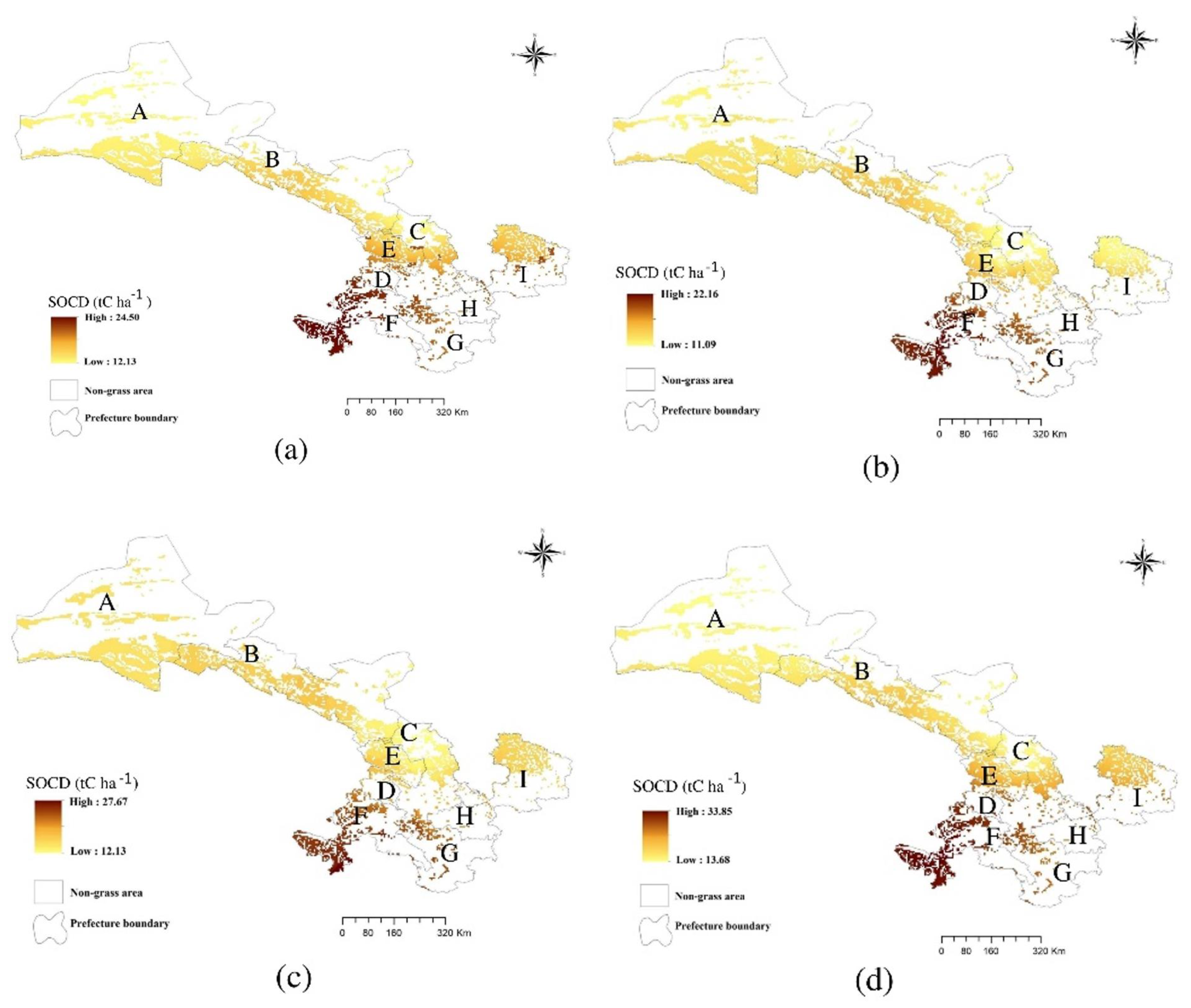
3.2.2. Spatial and Temporal Distribution of SOC and ABVG

Table 8. Zonal distribution of Gansu grassland carbon stock and vital statistics.

		Soil Organic Carbon Density (SOCD) t C/ha				SOC Storage (SOCS) (×106 t C)				Aboveground Biomass (ABVG) (g cm−2)
Zone	No. of Sites	Min	Max	Av	Std	Min	Max	Av	Std	Min	Max	Av	Std
A	8	5.23	12.67	8.67	1.89	11.61	19.73	16.66	6.14	7.2	250.34	80.69	72.14
B	12	7.52	15.55	10.4	2.03	15.96	34.91	30.44	5.04	90.89	234.56	125.24	34.33
C	12	9.38	17.45	13.4	2.44	30.46	35.05	34.86	1.25	300.5	790.78	500.25	149.22
D	4	10.45	20.23	15.53	3.01	25.76	45.42	45.46	5.71	275.34	1004.01	800.3	199.89
E	8	13.44	23.78	19.21	2.01	49.5	53.39	51.87	1.08	359.3	1575.05	900.45	384.18
F	7	16.55	30.68	23.17	4.21	95.7	112.5	89.62	4.15	464.34	1207.56	790.5	209.29
G	9	15.67	29.56	22.8	3.85	83.29	96.89	75.46	3.79	87.05	400.58	284.23	104.19
H	6	11.25	21.56	16.68	2.98	42.91	48.41	48.82	1.64	314.6	689.45	505.4	124.22
I	15	14.3	22.75	19.13	2.27	46.72	51.36	42.91	1.28	45.5	945.05	300.9	248.73

shows the summary statistics of the output variables for the various zones:

We grouped all the 81 study sites into nine zones (A to I) (Figure 1). Each zone has a specific number of sites. In each zone, we computed the average and standard deviation of SOC storage (SOCS) and ABVG. Zones F and G, both located in the southeast, have the most accumulated SOC. However, zone A in the northwest arid region had the least accumulated SOC. We also computed the average aboveground biomass and SOCD at intervals of at least 10 years for each site. We then interpolated the values to obtain a spatiotemporal map of the province. Figure 3 illustrates the SOCD dynamics in Gansu between 1968 and 2018 for 50 years.

Higher values of SOC density were estimated in the southeast throughout the simulation period. However, lower values of SOC were recorded in arid regions to the northwest. Generally, SOCD decreased from the southeast to the northwest. The average SOCD between 1979 and 1989 was lower than that of the previous decade, and increased afterward until 2018. Between 1968 and 2018, the average SOCD increased by 38% in parts of the southeast, whereas the increase in most parts of the northeast was approximately 9%. This is mainly due to the intensive land management simulated to fight desertification. In our model, we assumed intensive tilling to convert deserts into farmlands. This led to a tremendous release of SOC from the soil. However, after the 1980s, we simulated a no-till management practice and this led to a significant accumulation of SOC. In the alpine regions, SOC has always been on an increasing trend, as we simulated no-till land management practices throughout the period. Consequently, the soil was undisturbed and therefore accumulated SOC progressively, with the exception of Qingyang (zone I), where SOCD decreased from 1968 to 2000 and increased from 2000 to 2018. As a result, most of the SOC is concentrated in the southeast, especially in zones F and G (Figure 3).

We also estimated the amount of aboveground biomass for the study period. Figure 4 shows the spatial and temporal distribution of aboveground biomass between 1968 and 2018.

During the first decade, the aboveground biomass was relatively low, especially in zone I (Figure 4). Vegetation health in the northwest deteriorated in the second and third decades, but improved between 2000 and 2018. During this period, ABVG increased significantly, especially in the alpine regions. However, it deteriorated drastically again in zone I. In this zone, we simulated intensive erosion and consistent land tilling practices.

We calculated the percentage change in SOC between 1968 and 2018 of SOCS in all 81 sites to determine the SOC dynamics. We then interpolated the values using the Kriging interpolation method. Figure 5 shows the results.

As illustrated by Figure 5, the change in SOCD is not evenly distributed. The southeast and central parts accumulated more SOC than the northwest and zone I to the south. These areas of least increase underwent constant tilling and other anthropogenic interferences. As a result, SOC could not accumulate as much as it did in the southeast.

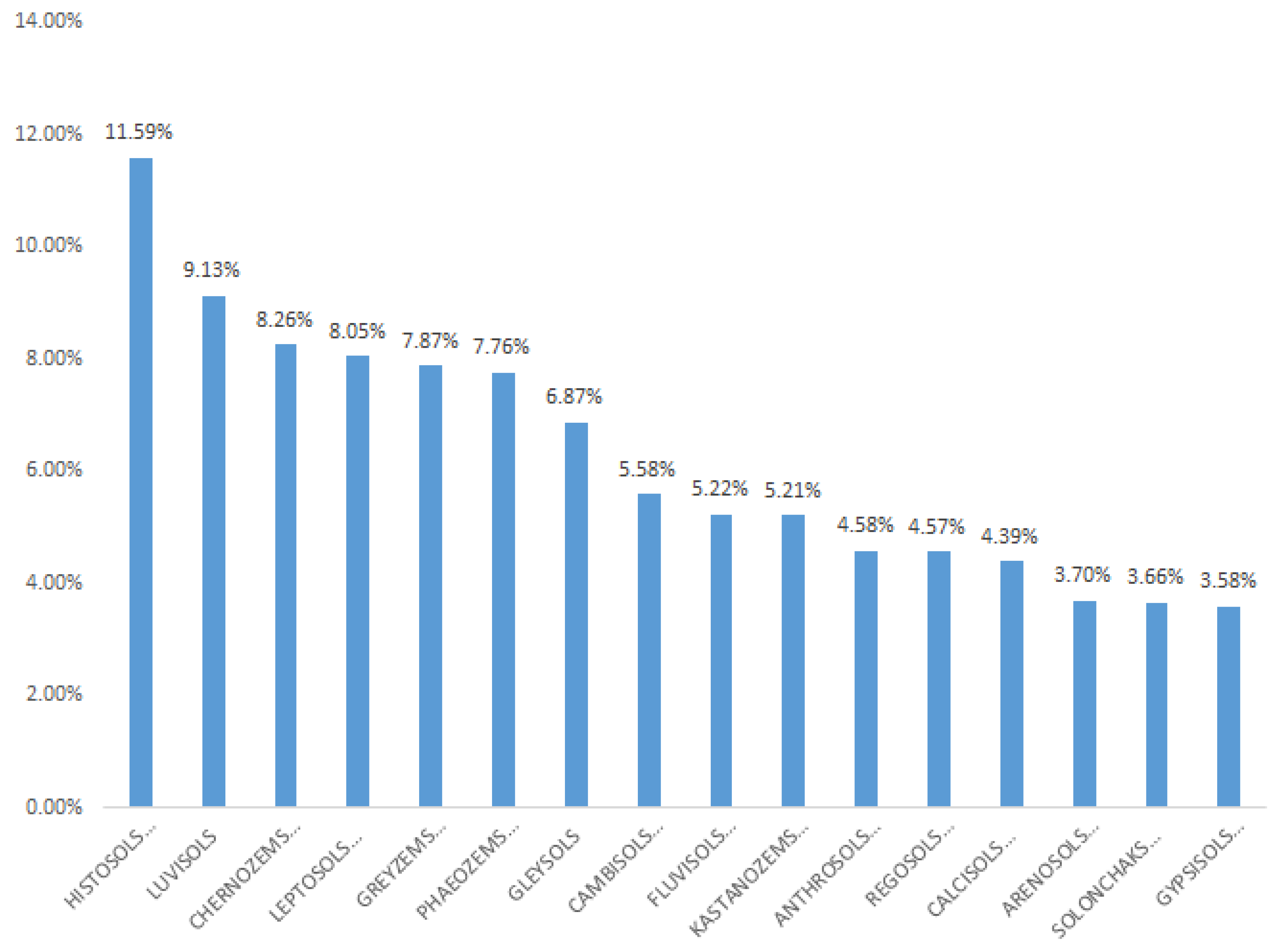
3.2.3. SOCD and ABCG Distribution by Soil Type

For each soil group, we computed the average SOCS and ABVG between 1968 and 2018 across all of the study sites. Figure 6 illustrates the distribution of SOCS and ABVG among the various soil types between 1968 and 2018.

Luvisols have the highest aboveground biomass, followed by Chernozems. In particular, Luvisols are found only in the southeastern part. In addition, Arenosols, Calcisols, and Anthrosols found in the northwest and the central part of the province have very low values of ABVG. There is also a huge variation in the distribution of ABVG among the various soil groups. Among the soil groups with the highest concentration of SOC are Histosols and Luvisols, localized in the Gannan alpine region. Following closely are Chernonozems, which are mainly found in the southeast, with very little coverage in the central part. Gypsisols and Solonchaks, found only in the northwest, have the least ABVG, followed by Calcisols, Arenosols, and Anthrosols, which are mostly localized in the northwest and central parts. It can be seen that extreme values of ABVG are found in soils that are localized in either the southeast or northwest. Soils found either throughout the province or only in the central part have values in between. Typical examples are Regosols, Phaeozems, and Kastanozems.

Among the soil groups, Hostosols sequestered the most SOC (52.33 × 10⁶ t C), representing 11.95% (Figure 7). Gypsisols, Solonchaks, and Arenosols altogether accounted for about 11% of C storage. This is mainly due to their low coverage and low SOCD.

Gypsisols, Solonchaks, Arenosols, and Calcisols each sequestered 17.44 × 10⁶ t C, representing 4% of the total SOC.

4. Discussion

We adapted the CENTURY model to the grasslands of Gansu and successfully estimated the amount of carbon sequestered in the soils (0–20 cm), as well as the aboveground biomass. Our measured and observed SOCD and ABVG had correlation coefficients of 0.76 and 0.50, respectively, at p < 0.01 (Table 6 and Table 7). Histosols had the highest SOC sequestration rate (25 t C/ha), with Gypsisols having the least (7.8 t C/ha). Aboveground biomass ranged from 0.002 to 1.130 kg C m⁻² among the 16 soil types across the province (Figure 5). The average aboveground biomass density estimated was 2.95 × 102 0.415 ± 1.15 × 102 g C/m², which was consistent with Xu et al. (0.69 ± 0.20 kg C m⁻²) [41]. Precipitation was correlated with SOC and aboveground biomass with a correlation efficiency of 0.57 and 0.89, respectively, at p < 0.01.

Compared with other regional studies, the SOCD of Gansu is lower than the average value of 48.6 t C ha⁻¹ in the arid region in Western China [17]. This suggests that the grasslands of Gansu Province have a huge SOC sequestration potential. Our findings are consistent with the majority of SOC studies in the province and its environs. For example, Guo et al. [42] estimated the grassland SOCD in Inner Mongolia to be 19.9 t C/ha, a value within our estimated values in Gansu. According to their study, SOC values were higher in the southeast (21.56 t C/ha) but lower in the northwest (13.77 t C/ha) part of Gansu Province, a pattern we also discovered in our study.

The spatial distribution of the aboveground biomass was similar to that of the SOC density (Figure 4 and Figure 5). The aboveground biomass and SOC densities declined from the southeast to the northwest. The majority of the soils found in the south are relatively fertile (Catling D., 1992) [43], giving rise to huge variations in SOC and ABVG distributions. Another reason could be from the differences in management practices and soil properties, such as the pH. The function of pH in biomass production cannot be overemphasized. Neina, D. (2019) [44] refers to soil pH as the master soil variable, observing that it controls the solubility, mobility, and bioavailability of trace elements, which determines their translocation in plants. It also affects the soil enzymes and microbial activities (Marinos, R. and Bernhardt, E.) [45], as well as biodegradation. Therefore, in our model, we placed special emphasis on the variation of pH among the various soils. According to Neina, McCauley, and 2009 [46], D. (2019) [47] the activities of soil microorganisms and crop growth are the greatest near neutral conditions, but the pH ranges vary for each type of microorganism and plant. They claim that very acidic soils (less than 5) cause microbial activities and numbers to be considerably lower than in the soils that are more neutral [46]. According to esf.edu [47], most minerals and nutrients are more soluble or available in acid soils than in neutral or slightly alkaline soils, but adds that optimum pH conditions for individual crops will vary. In their research, Zhou, et al. (2019) [48] observed that soil carbon is negatively correlated with soil pH, demonstrating that relatively low pH benefits the accumulation of organic matter. According to McCauley, A., Jones, C., and Jacobsen, J. (2009) [46], soil pH strongly affects soil functions and plant nutrient availability by influencing the chemical solubility and availability of the plant essential nutrients, as well as the organic matter decomposition.

The majority of soils in the province have optimal levels of pH 5–8 for plant growth (Table 1). For instance, the northwestern part is dominated by Euteric soils, which are neutral to slightly acid, with a good availability of nutrients, fine texture, moderate to high cation exchange capacity, and low to moderate organic matter content, and the natural fertility is fairly high [43].

Soils in the northwest have the right level of pH for plant growth, much like soils in the southeast. However, the positive effect of pH is nullified by the absence of sufficient plants. For example, Marinos and Bernhardt (2018) [45] found that microbial respiration and SOC solubility were strongly stimulated by increased soil pH, but only in the presence of plants, stating that a soil pH increase of 0.76 units increased soil respiration by 19% in the organic soil horizon and 38% in the mineral soil horizon, whereas in unplanted pots, soil pH had no effect on microbial respiration. The presence of the right pH alone cannot trigger plant growth. They observed that while increased soil pH enhanced plant-mediated heterotrophic respiration, it had no effect on plant growth. In contrast, soil Ca enrichment increased the relative growth rate of plants by 22%, but had no impact on microbial respiration. Plant biomass is higher in the southeast, because the majority of the soils are Ca rich. We therefore suggest that policy-makers lay special emphasis on enriching the calcium content of soils in the northwest of the province to facilitate plant growth.

Another major factor inhibiting plant growth in the northwest is the climate. Xu et al., 2018 [41], found that precipitation positively correlated with vegetation biomass and SOC, whereas temperature was negatively correlated with SOC. The northwestern part of the province has very low precipitation, thereby affecting vegetation biomass production. These factors lead to low SOC and vegetation biomass [46] in the northwest. The low amount of precipitation in the northwest also leads to little leaching of base cations, resulting in a relatively high degree of base saturation [46]. According to the same author, cation and anion exchange capacity (the soil’s ability to retain and supply nutrients to a crop) is directly affected by soil pH. When the soil pH is high (i.e., low concentration of H+), more base cations will be on the particle exchange sites and will thus be less susceptible to leaching. An increase in precipitation causes increased leaching of base cations and the soil pH is lowered [46]. However, when the soil pH is lower (i.e., higher concentration of H+), more H+ ions are available to “exchange” the base cations, thereby removing them from exchange sites and releasing them into the soil water. As a result, exchanged nutrients are either taken up by the plant or lost through leaching or erosion. The southeastern part is dominated by Calcaric soils and some amount of Euteric soils. Calcaric means the presence of calcium carbonate. They have high natural fertility but are potentially alkaline [43]. According to Céspedes-Payret et al. (2017) [49], bulk density values are not significantly correlated with SOC content. Our model could not predict aboveground biomass as much as it did SOC because of the inherent problem of the century model not being able to model the finer timescale of ABVG accumulation. Our finding also indicates that precipitation affects aboveground biomass more than it does SOC.

Another factor contributing to the spatial variation is differences in climate. The southeastern part of the province has more conducive conditions for plant growth than the northwest. For example, rainfall increases from the northwest to the southeast. However, temperature decreases in the same direction. The northwestern part is icy cold throughout most of the year. According to Xu et al., 2018 [41], the main factors that affect the spatial distribution of aboveground biomass are climate and soil nutrients. They observed that these factors account for 68.16% of the total variation in aboveground biomass in a GLM analysis. Among these factors, climate was the most important influencing factor, explaining 50.49% of the total variance. In addition, they observed that soil texture plays a significant role in the total variance in the spatial patterns of SOC density for the 0–20 cm soil layers. The climate of Gansu Province is very diverse and, therefore, precipitation and temperatures vary greatly [29]. The century model was able to account for the variation in precipitation and temperature, and showed that carbon density was influenced greatly by climate. The aboveground biomass density was generally higher in high-precipitation areas. The temperate arid regions had the lowest aboveground biomass density. High values of aboveground biomass were estimated in the southeastern part compared with the northwest part. Nevertheless, the amount of ABVG simulated by our model in the northwest was greater than the measured values. We attribute this to the overgeneralization of parameters and conditions throughout the simulation. Most SOC was concentrated in the alpine regions. The arid regions, located in the northwest, had the lowest SOC density at 0–20 cm. This was consistent with the findings of Xu et al., 2018 [41].

Between 1968 and 2018, the entire region was a carbon sink and since then, the SOC has been on a gradual incline. Beginning in 1968, the SOC showed a sharp decrease, but began to increase in 1971 and has been increasing annually. The southeastern part saw a rather gradual increase in SOCD, while the majority of the decrease took place in the arid regions and the central part of the province. Even though the province has generally been a carbon sink for the past 50 years, a few areas have been shown to lose SOC. This was mainly due to overgrazing and other management practices, which our model accounted for. For instance, zones A, B, and I (Figure 1 and Figure 4) lost aboveground biomass rapidly due to extensive land tilling (National Research Council, 1992) [50,51]. The FAO observed that soil loss due to wind erosion was 10 to 15 cm and sand loss was 20 to 150 cm in the northwest [51]. Therefore, our model was calibrated to simulate more erosion in the arid regions. According to FAO and historical records, overgrazing accounts for over 20% of decertified areas. The incorporation of intensive grazing into our simulation contributed to its accuracy. However, low-intensity grazing was simulated between 1988 and 1998. During this period, the government established plantations for desertification control and measures were put in place to regulate grazing [51].

According to Xu et al., 2011 [52], there has been a large-scale reclamation of arid land in Northwest China over the past 50 years, converting the natural desert landscape into an anthropogenic oasis. SOC is greatly influenced by anthropogenic activities (Breuer et al., 2006 [53], and Kasel and Bennett, 2007 [54]). Therefore, Xu et al., 2011, speculate that drastic human activities may have caused the radical change in SOC. As a result, we observed a relatively stable increase in SOC in the alpine regions than in areas influenced by human activities. In arid regions, we found that SOC storage decreased most of the time between 1968 and 2000, and gradually increased afterward. The rapid loss of SOC in semi-arid regions under cultivation has been reported by several researchers. For example, Elberling et al. (2003) [55] reported that up to 24% of SOC in the upper 1 m layer has been lost over the 40 years since the Savannah began to be cultivated in semiarid Senegal in West Africa. Similarly, Ogle et al. (2004) [56] observed that the level of SOC in tropical regions was reduced to 32% due to a 20-year tillage. A similar phenomenon was observed by Su et al. (2004) [57] in the semiarid Horqin sandy steppe of northern China. They also observed that in just 3 years of cultivation, sandy grassland lost up to 38% of SOC. In most of these instances, the loss was rapid within the first few years, as it was in the case of the Nigerian semiarid Savannah. (Jaiyeoba, 2003) [58].

Our model was not without flaws. These were partly due to inevitable assumptions and the oversimplification of reality. We did not account for land cover change over the research period, for example. The area of grassland used could only match that in 2010 and therefore did not account for the change. Secondly, the monthly timeframe of the century model fails to adequately depict the precise timescale of biomass growth (Yu et al., 2014) [59]. This undoubtedly affected the biomass and SOC stock estimation. Furthermore, as shown in the literature, the chemical properties of the same soil in various places might differ dramatically. Wherever necessary, we used the average values across all of the areas where those soils were found. A major drawback faced was the fact that at most sites, historical data were hard to find, especially data on management practices such as fertilization and irrigation. In such circumstances, we used our discretion based on extant management practices in those areas. Another instance of oversimplification of reality is the model’s failure to account for altitude. Altitude affects vegetative carbon and SOC, according to Xu et al., 2018 [41]. They observed that vegetation carbon declined with altitude, whereas SOC density increased with increasing latitude. Wang et al. [60] also observed a similar pattern in China. However, the CENTURY model does not account for this important factor. Other researchers such as Oelbermann have also found some operational problems with the model. They found that the model estimated lower SOC than the measured SOC values because it failed to account for changes in soil bulk density [61].

We recommend CENTURY developers include the effects of altitude in order to increase the model’s estimation accuracy. We also recommend that authorities in charge give attention to Ca modification practices, especially in the northwest, alongside intensive plant growth. In addition, Slaton et al., 2001 [62], and McCauley, A., Jones, C., and Jacobsen, J. (2009) [46] suggest the addition of amendments to soils to modify the soil pH. Suggested amendments are elemental sulfur, ferrous sulfate (FeSO4), aluminum sulfate (Al₂(SO₄)₃), ammonium (NH₄+)-based fertilizers, soil organic matter (SOM), and NH4+-based fertilizers. The acidifying effects of fertilization may be more than compensated for by other land use practices. For instance, a study by Jones, C.A., J. Jacobsen, and S. Lorbeer, 2002 [63], found that over a 20-year period, fertilized and cultivated soils in Montana experienced, on average, higher pH values than non-fertilized/non-cultivated soils. They explained that in fertilized/cultivated soils, practices such as crop removal during harvest and tilling decrease SOM levels and subsequent acid production. Additionally, tillage increases surface and sub-surface soil mixing, moving CaCO₃ from the sub-surface closer to the soil surface.

5. Conclusions

The application of the CENTURY model to simulate the SOC dynamics in Gansu Province was successful. Over the past 50 years, the region has been a carbon sink for the most part. However, intensive grazing and anthropogenic activities in the arid regions made the area a slight carbon source in the early years of the simulation. The region became a carbon sink due to government interventions after the second part of the simulation. We estimated that the grasslands of Gansu stored 436.098 × 106 ± 87.25 × 104 t C of soil SOC at 0–20cm, and accounted for about 0.468% of the total national SOC carbon inventory and 1.54% of the total national grassland SOC stock. We also estimated an average SOC density of 15.75 t C/ha across the province. The most carbon is sequestered in the alpine and southeastern regions of the province.

The SOC sequestration potential differs among the soil types. For instance, Histosols sequestered the most amount of SOC, followed by Luvislols and Chernozems, all of which are found mostly in the south. Gypsisols, Solonchaks, and Arenosols, all found in the northwest, sequestered the least SOC. For the past 50 years, the province has been a carbon sink. However, a few areas were shown to lose SOC. The SOC loss was mainly due to overgrazing and other management practices. In general, our estimated SOCD was less than the national average, indicating the grassland of the province has a huge carbon sequestration potential.

References

1. Masson-Delmotte, V.; Zhai, P.; Pörtner, H.O.; Roberts, D.; Skea, J.; Shukla, P.R.; Pirani, A.; Moufouma-Okia, W.; Péan, C.; Pidcock, R.; et al. Global Warming of 1.5 °C. An IPCC Special Report on the Impacts of Global Warming of 1.5 °C above pre Industrial Levels and Related Global Greenhouse Gas Emission Pathways, in the Context of Strengthening the Global Response to the Threat of Climate Change, Sustainable Development, and Efforts to Eradicate Poverty; IPCC: Geneva, Switzerland, 2018. [Google Scholar]
2. Han, R.Q.; Zhen, D.; Dai, E.F.; Wu, S.H.; Zhao, M.H. Response of production potential to climate fluctuation in major grain regions of China. Resour. Sci. 2014, 36, 2611–2623. [Google Scholar]
3. Cline, W.R. The impact of global warming of agriculture: Comment. Am. Econ. Rev. 1996, 86, 1309–1311. [Google Scholar]
4. Tanaka, S.K.; Zhu, T.; Lund, J.R.; Howitt, R.E.; Jenkins, M.W.; Pulido, M.A.; Tauber, M.; Ritzema, R.S.; Ferreira, I.C. Climate warming and water management adaptation for California. Clim. Chang. 2006, 76, 361–387. [Google Scholar] [CrossRef]
5. Yang, X.M. Using agricultural soils to fix organic carbon—Alleviating global warming and improving soil productivity. Soil Environ. Sci. 2000, 9, 311–315. [Google Scholar]
6. Yang, X.M.; Zhang, X.P.; Fang, H.J. The significance of carbon sequestration in agricultural soils to alleviate global warming. Sci. Geogr. Sin. 2003, 23, 101–106. [Google Scholar]
7. Intergovernmental Panel on Climate Change. Climate Change 1995: Impact, Adaptation and Mitigation: Scientific Technical Analyses; Working Group 1; Cambridge University Press: Cambridge, UK, 1996. [Google Scholar]
8. Lal, R. Soil Erosion and Gaseous Emissions. Appl. Sci. 2020, 10, 2784. [Google Scholar] [CrossRef] [Green Version]
9. Sornpoon, M.; Bonnet, S.; Garivait, S. Effect of open burning on soil carbon stock in sugarcane plantation in Thailand. World Acad. Sci. Eng. Technol. 2014, 8, 822–827. [Google Scholar]
10. Ray, R.L.; Griffin, R.W.; Fares, A.; Elhassan, A.; Awal, R.; Woldesenbet, S.; Risch, E. Soil CO2 emission in response to organic amendments, temperature, and rainfall. Sci. Rep. 2020, 10, 5849. [Google Scholar] [CrossRef] [Green Version]
11. Wang, K.F. Coupling Development of Triple-Microbe Model and Its Simulation of Global Soil Organic Carbon and Microbial Carbon; Northwest A & Forestry University: Xianyang, China, 2017. [Google Scholar]
12. Bohn, H.L. Estimate of organic carbon in world soils. Soil Sci. Soc. Am. J. 1982, 46, 1118–1119. [Google Scholar] [CrossRef]
13. Jobbágy, E.G.; Jackson, R.B. The vertical distribution of soil organic carbon and its relation to climate and vegetation. Ecol. Appl. 2000, 10, 423–436. [Google Scholar] [CrossRef]
14. Wang, S.Q.; Zhou, C.H. Estimating soil organic carbon reservoir of terrestrial ecosystem in China. Geogr. Res. 1999, 18, 349–356. [Google Scholar]
15. Luo, W.; Zhang, H.H.; Chen, J.J.; Liu, Y.; Li, D.Q. Storage and spatial distribution of soil organic carbon in Guangdong Province. Ecol. Environ. Sci. 2018, 27, 1593–1601. [Google Scholar]
16. Han, B.; Wang, X.K.; Ou, Y.Z.Y. Distribution and change of agro-ecosystem carbon pool in Northeast of China. Chin. J. Soil Sci. 2004, 35, 1140–1147. [Google Scholar]
17. Zhang, J.; Lin, M.; Ao, Z.Q. Estimation of soil organic carbon storage in arid areas of Western China. J. Arid Area Resour. Environ. 2018, 32, 132–137. [Google Scholar]
18. Yang, A.G.; Miao, Z.H.; Qiu, F.F.; Yang, Q.C.; Wang, Z.M.; Mao, D.H. Estimation and spatial distribution of organic carbon storage in topsoil of Sanjiang Plain based on GIS. Bull. Soil Water Conserv. 2015, 35, 155–158. [Google Scholar]
19. Xiao, X.M.; Wang, Y.F.; Chen, Z.Z. Dynamics of primary productivity and soil organic matter of typical steppe in the Xilin River Basin of Inner Mongolia and their responses to climate change. J. Integr. Plant Biol. 1996, 38, 45–52. [Google Scholar]
20. Zhang, Y.Q.; Tang, Y.H.; Jiang, J. Dynamic characteristics of soil organic carbon in grassland ecosystems of the Qinghai-Tibet Plateau. Sci. Sin. 2006, 36, 1140–1147. [Google Scholar]
21. Althoff, T.D.; Menezes, R.S.C.; Pinto, A.D.S.; Pareyn, F.G.C.; Carvalho, A.L.D.; Martins, J.C.R.; Carvalho, E.X.D.; Silva, A.S.A.D.; Dutra, E.D.; Sampaio, E.V.D.S.B. Adaptation of the CENTURY model to simulate C and N dynamics of Caatinga dry forest before and after deforestation. Agric. Ecosyst. Environ. 2018, 254, 26–34. [Google Scholar] [CrossRef]
22. Tang, M.; Wang, S.; Zhao, M.; Falyu, Q.; Liu, X. Simulated Soil Organic Carbon Density Changes from 1980 to 2016 in Shandong Province Dry Farmlands Using the CENTURY Model. Sustainability 2020, 12, 5384. [Google Scholar] [CrossRef]
23. Available online: https://www.chinadaily.com.cn/m/gansu/2013-10/24/content_17055494.htm (accessed on 15 February 2020).
24. Kottek, M.; Grieser, J.; Beck, C.; Rudolf, B.; Rubel, F. World map of the Köppen-Geiger climate classification updated. Meteorol. Z. 2006, 15, 259–263. [Google Scholar] [CrossRef]
25. Nachtergaele, F.; van Velthuizen, H.; Verelst, L.; Batjes, N.H.; Dijkshoorn, K.; van Engelen, V.W.P.; Fischer, G.; Jones, A.; Montanarella, L.; Petri, M. The harmonized world soil database. In Proceedings of the 19th World Congress of Soil Science, Soil Solutions for a Changing World, Brisbane, Australia, 1–6 August 2010; pp. 34–37. [Google Scholar]
26. Driessen, P.; Deckers, J.; Spaargaren, O.; Nachtergaele, F. Lecture Notes on the Major soils of the World; Food and Agriculture Organization (FAO): Rome, Italy, 2000. [Google Scholar]
27. Harmonized World Soil Database Version 1.2 (HWSD V1.2). Available online: http://www.fao.org/soils-portal/data-hub/soil-maps-and-databases/harmonized-world-soil-database-v12/en/ (accessed on 6 January 2020).
28. Available online: http://www.ecosystem.csdb.cn/ (accessed on 1 August 2020).
29. Available online: www.worldclim.org (accessed on 20 March 2020).
30. Pattern, N.C.S. Climatic Research Unit, University of East Anglia. Available online: https://crudata.uea.ac.uk/cru/data/ncp (accessed on 10 August 2020).
31. Available online: http://koeppen-geiger.vu-wien.ac.at/present.htm (accessed on 15 February 2020).
32. Rusong, W. The frontiers of urban ecological research in industrial transformation. Acta Ecol. Sin. 2000, 20, 830–840. [Google Scholar]
33. Shi, X.Z.; Yu, D.S.; Warner, E.D.; Pan, X.Z.; Petersen, G.W.; Gong, Z.G.; Weindorf, D.C. Soil database of 1:1,000,000 digital soil survey and reference system of the Chinese genetic soil classification system. Soil Surv. Horiz. 2004, 45, 129–136. [Google Scholar] [CrossRef]
34. Kodešová, R.; Alias, L.J. Available online: http://www.koedoe.co.za (accessed on 10 August 2020).
35. Spawn, S.A.; Gibbs, H.K. Global Aboveground and Belowground Biomass Carbon Density Maps for the Year 2010. ORNL DAAC 2020. [Google Scholar] [CrossRef]
36. Parton, W.J. The CENTURY Model. In Evaluation of Soil Organic Matter Models; Springer: Berlin/Heidelberg, Germany, 1996; pp. 283–291. [Google Scholar]
37. Available online: https://www.nrel.colostate.edu/projects/century/ (accessed on 10 June 2020).
38. Bortolon, E.S.O.; Mielniczuk, J.; Tornquist, C.G.; Lopes, F.; Bergamaschi, H. Validation of the Century model to estimate the impact of agriculture on soil organic carbon in Southern Brazil. Geoderma 2011, 167, 156–166. [Google Scholar] [CrossRef]
39. Bockstaller, C.; Girardin, P. How to validate environmental indicators. Agric. Syst. 2003, 76, 639–653. [Google Scholar] [CrossRef]
40. Gomes, A.G.; Varriale, M.C. Modelagem de Ecossistemas, Uma Introducao; UFSM: Santa Maria, Brazil, 2004. [Google Scholar]
41. Xu, L.; Yu, G.; He, N.; Wang, Q.; Gao, Y.; Wen, D.; Li, S.; Niu, S.; Ge, J. Carbon storage in China’s terrestrial ecosystems: A synthesis. Sci. Rep. 2018, 8, 1–13. [Google Scholar] [CrossRef]
42. Guo, L.H.; Gao, J.B.; Wu, S.H.; Hao, C.Y.; Zhao, D.S. Spatial-temporal change of soil organic carbon and its susceptibility to climate change in Inner Mongolia Grassland 1981–2010. Res. Environ. Sci. 2016, 29, 1050–1058. [Google Scholar]
43. Catling, D. The Soils. In Rice in Deep Water; Palgrave Macmillan: London, UK, 1992. [Google Scholar] [CrossRef]
44. Neina, D. The Role of Soil pH in Plant Nutrition and Soil Remediation. Appl. Environ. Soil Sci. 2019, 2019, 1–9. [Google Scholar] [CrossRef]
45. Marinos, R.E.; Bernhardt, E.S. Soil carbon losses due to higher pH offset vegetation gains due to calcium enrichment in an acid mitigation experiment. Ecology 2018, 99, 2363–2373. [Google Scholar] [CrossRef]
46. McCauley, A.; Jones, C.; Jacobsen, J. Soil pH and organic matter. Nutr. Manag. Module 2009, 8, 1–12. [Google Scholar]
47. Available online: https://www.esf.edu/pubprog/brochure/soilph/soilph.htm (accessed on 10 March 2021).
48. Zhou, W.; Han, G.; Liu, M.; Li, X. Effects of soil pH and texture on soil carbon and nitrogen in soil profiles under different land uses in Mun River Basin, Northeast Thailand. Peer J. 2019, 7, e7880. [Google Scholar] [CrossRef] [Green Version]
49. Céspedes-Payret, C.; Bazzoni, B.; Gutiérrez, O.; Panario, D. Soil organic carbon vs. bulk density following temperate grassland afforestation. Environ. Process. 2017, 4, 75–92. [Google Scholar] [CrossRef]
50. National Research Council. Grasslands and Grassland Sciences in Northern China; National Academies Press: Washington, DC, USA, 1992. [Google Scholar]
51. Overview of Land Desertification Issues and Activities in the People’s Republic of China. Available online: http://www.fao.org/3/w7539e/w7539e03.htm (accessed on 12 March 2020).
52. Xu, W.; Chen, X.; Luo, G.; Lin, Q. Using the CENTURY model to assess the impact of land reclamation and management practices in oasis agriculture on the dynamics of soil organic carbon in the arid region of North-western China. Ecol. Complex. 2011, 8, 30–37. [Google Scholar] [CrossRef]
53. Breuer, L.; Huisman, J.; Keller, T.; Frede, H.-G. Impact of a conversion from cropland to grassland on C and N storage and related soil properties: Analysis of a 60-year chronosequence. Geoderma 2006, 133, 6–18. [Google Scholar] [CrossRef]
54. Kasel, S.; Bennett, L. Land-use history, forest conversion, and soil organic carbon in pine plantations and native forests of south eastern Australia. Geoderma 2007, 137, 401–413. [Google Scholar] [CrossRef]
55. Elberling, B.; Touré, A.; Rasmussen, K. Changes in soil organic matter following groundnut–millet cropping at three locations in semi-arid Senegal, West Africa. Agric. Ecosyst. Environ. 2003, 96, 37–47. [Google Scholar] [CrossRef]
56. Ogle, S.M.; Conant, R.T.; Paustian, K. Deriving grassland management factors for a carbon accounting method developed by the intergovernmental panel on climate change. Environ. Manag. 2004, 33, 474–484. [Google Scholar] [CrossRef] [PubMed]
57. Su, Y.Z.; Zhao, H.l. Soil properties and plant species in an age sequence of Caragana microphylla plantations in the Horqin Sandy Land, north China. Ecol. Eng. 2003, 20, 223–235. [Google Scholar] [CrossRef]
58. Jaiyeoba, I.A. Changes in soil properties due to continuous cultivation in Nigerian semiarid Savannah. Soil Tillage Res. 2003, 70, 91–98. [Google Scholar] [CrossRef]
59. Yu, S.S.; Dou, S.; Yang, J.M. Application of central model in soil organic carbon research. Soils Crop. 2014, 3, 10–14. [Google Scholar]
60. Wang, S.Q. Analysis on spatial distribution characteristics of soil organic carbon reservoir in China. Acta Geogr. Sin. 2000, 55, 533–544. [Google Scholar]
61. Oelbermann, M.; Voroney, R.P. An evaluation of the century model to predict soil organic carbon: Examples from Costa Rica and Canada. Agrofor. Syst. 2011, 82, 37–50. [Google Scholar] [CrossRef]
62. Slaton, N.A.; Norman, R.J.; Gilmour, J.T. Oxidation rates of commercial elemental sulfur products applied to an alkaline silt loam from Arkansas. Soil Sci. Soc. Am. J. 2001, 65, 239–243. [Google Scholar] [CrossRef]
63. Jones, C.A.; Jacobsen, J.; Lorbeer, S. Metal concentrations in three Montana soils following 20 years of fertilization and cropping. Commun. Soil Sci. Plant Anal. 2002, 33, 1401–1414. [Google Scholar] [CrossRef]
Figure 1. Gansu Province, China, indicating study sites (validation points). (A) Jiayuguan, Aksai Kazakh, Anxi, Dunhuang, Jinta, Subei Mongol, Suzhou, and Yumen; (B) Jinchuan, Yongchang, Heshui, Minqin, Tianzhu Tibetan, Wuwei, Gaotai, Linze, Minle, Shandan, Sunan Yugur, and Zhangye; (C) Baiyin, Huining, Jingtai, Jingyuan, Pingchuan, Dingxi, Lintao, Longxi, Min, Tongwei, Weiyuan, and Zhang; (D) Gaolan Liangzhou, and Yongdeng Yuzhong; (E) Dongxiang, Guanghe, Hezheng (Linxia), Jishishan Bonan, Kangle, Linxia Shi, Linxia, and Yongjing; (F) Zhuoni, Lintan, Luqu, Maqu, Diebu, Xiahe, and Zhugqu; (G) Cheng, Dangchang, Hui, Kang, Liangdang, Li, Wen, Wudu, and Xihe; (H) Gangu, Qin’an, Qingcheng, Tianshui, Wushan, and Zhangjiachuan Hui; (I) Chongxin, Huating, Jingchuan, Jingning, Lingtai, Pingliang, Zhuanglang, Hezheng (Qingyang), Huachi, Huan, Ning, Qingyang, Xifeng, Zhengning, and Zhengyuan.
Sustainability 13 09434 g001
Figure 2. Flowchart of the model calibration, parameterization, and simulation.
Sustainability 13 09434 g002
Figure 3. Spatial and temporal distribution of SOC of the grasslands of Gansu from 1968 to 2018: (a) 1968 to 1978, (b) 1979 to 1989, (c) 1990 to 2000, and (d) 2001 to 2018.
Sustainability 13 09434 g003
Figure 4. Spatial and temporal distribution of the aboveground biomass in the grasslands of Gansu from 1968 to 2018: (a)1968 to 1978, (b) 1979 to 1989, (c) 1990 to 2000, (d) 2001 to 2018.
Sustainability 13 09434 g004
Figure 5. Percentage change in SOCD in Gansu grasslands between 1968 and 2018.
Sustainability 13 09434 g005
Figure 6. SOC distribution of SOC and aboveground biomass by grassland type.
Sustainability 13 09434 g006
Figure 7. Percentage distribution of SOCS by soil type in Gansu Province, China, between 1968 and 2018.
Sustainability 13 09434 g007