Article

Predictive Innovative Methods for Aquatic Heavy Metals Pollution Based on Bioindicators in Support of Blue Economy in the Danube River Basin

by
Ira-Adeline Simionov
1,*,
Dragoș Sebastian Cristea
2,
Ștefan-Mihai Petrea
3,*,
Alina Mogodan
3,
Roxana Jijie
4,
Elena Ciornea
5,
Mircea Nicoară
5,
Maria Magdalena Turek Rahoveanu
6 and
Victor Cristea
1
1
Multidisciplinary Research Platform (ReForm)-MoRAS Research Center, “Dunărea de Jos” University of Galaţi, 800008 Galați, Romania
2
Faculty of Economics and Business Administration, “Dunărea de Jos” University of Galaţi, 800008 Galaţi, Romania
3
Department of Food Science, Food Engineering, Biotechnology and Aquaculture, Faculty of Food Science and Engineering, “Dunărea de Jos” University of Galaţi, 800008 Galați, Romania
4
Department of Exact and Natural Sciences, Institute for Interdisciplinary Research, “Alexandru Ioan Cuza” University of Iasi, 700107 Iasi, Romania
5
Department of Biology, Faculty of Biology, “Alexandru Ioan Cuza” University of Iasi, 700505 Iasi, Romania
6
Faculty of Engineering and Agronomy in Braila, “Dunărea de Jos” University of Galaţi, 810017 Braila, Romania
*
Authors to whom correspondence should be addressed.
Sustainability 2021, 13(16), 8936; https://doi.org/10.3390/su13168936
Submission received: 31 May 2021 / Revised: 23 July 2021 / Accepted: 2 August 2021 / Published: 10 August 2021

Abstract

:
Heavy metal pollution is still present in the Danube River basin, due to intensive naval and agricultural activities conducted in the area. Therefore, continuous monitoring of this pivotal aquatic macro-system is necessary, through the development and optimization of monitoring methodologies. The main objective of the present study was to develop a prediction model for heavy metals accumulation in biological tissues, based on field gathered data which uses bioindicators (fish) and oxidative stress (OS) biomarkers. Samples of water and fish were collected from the lower sector of Danube River (DR), Danube Delta (DD) and Black Sea (BS). The following indicators were analyzed in samples: cadmium (Cd), lead (Pb), iron (Fe), zinc (Zn), copper (Cu) (in water and fish tissues), respectively, catalase (CAT), superoxide dismutase (SOD), glutathione peroxidase (GPx), malondialdehyde (MDA) (in fish tissues). The pollution index (PI) was calculated to identify the most polluted studied ecosystem, which revealed that Danube River is seriously affected by the presence of Fe (IP = 4887) and strongly affected by the presence of Zn (IP = 4.49). The concentration of Cd in fish muscle tissue was above the maximum permitted level (0.05 µg/g) by the EU regulation. From all analyzed OS biomarkers, MDA registered the highest median values in fish muscle (145.7 nmol/mg protein in DR, 201.03 nmol/mg protein in DD, 148.58 nmol/mg protein in BS) and fish liver (200.28 nmol/mg protein in DR, 163.67 nmol/mg protein, 158.51 nmol/mg protein), compared to CAT, SOD and GPx. The prediction of Cd, Pb, Zn, Fe and Cu in fish hepatic and muscle tissue was determined based on CAT, SOD, GPx and MDA, by using non-linear tree-based RF prediction models. The analysis emphasizes that MDA in hepatic tissue is the most important independent variable for predicting heavy metals in fish muscle and tissues at BS coast, followed by GPx in both hepatic and muscle tissues. The RF analytical framework revealed that CAT in muscle tissue, respectively, MDA and GPx in hepatic tissues are most common predictors for determining the heavy metals concentration in both muscle and hepatic tissues in DD area. For DR, the MDA in muscle, followed by MDA in hepatic tissue are the main predictors in RF analysis.

1. Introduction

The Romanian Danube River basin, especially the lower sector, represents the basis for developing the country’s blue growth potential, to align to the European Union average performance registered by the blue economy sector. Therefore, the living resources subsector must be developed, while assuring both the safety and security of aquatic food products. However, this objective can pose a real challenge to achieve since in the lower sector of the Romanian Danube River (LRDR) basin several important economic/anthropogenic activities related to shipyard industry (in the area of Brăila, Galați and Tulcea city), steel industry (Galați county), alumina industry (Tulcea county) and intensive agricultural activity (especially in Brăila and Tulcea county) are present. Thus, all the activities generate significant concentrations of heavy metals released in the nearby environment, creating a risk of heavy metal accumulation in the aquatic ecosystem, situation which requires periodic pollution monitoring activities. Additionally, the LRDR connects to the Black Sea through the Danube Delta and if pollution occurs upstream of the river, the negative effects of this phenomenon can extend on the Romanian Black Sea and Danube Delta coastal areas as well.
According to [1], the coastal area accumulates large quantities of metals from agricultural and industrial activities. Fish are often used as bioindicators for water pollution caused by heavy metals [2,3,4], through fish liver analysis. Furthermore, the Regional Organization for the Protection of the Marine Environment recommends the use of fish as environmental monitoring tools [5]. According to [3], machine learning based models for the detection of heavy metals in aquatic environments are increasing the economic efficiency of monitoring campaigns conducted to identify the ecological status of surface waters and, additionally, the health risk that is associated with the ingestion of heavy metals after fish consumption.
Fish stocks are key components in the development of a blue economy based on marine living resources. Thus, fish meat analysis must be performed to verify food safety in terms of heavy metal concentration. However, heavy metal analysis involves a high financial cost, complex logistics and the development of complex working protocols [3]. In addition, since heavy metals are not equally distributed in the aquatic environment and the identifications of hot spots imply the collection of many samples for analysis, the monitoring campaigns are cost-demanding. Therefore, even though ecotoxicological mathematical models were performed to predict internal concentrations of organic chemicals in fish [6], more recent studies recommend the continual development and upgrade of these models [7].
The oxidative stress (OS) biomarkers analysis is less expensive and offers information related to fish welfare status.
Manifestation of the OS within an organism occurs due to the disparity between the production of reactive oxygen species (ROS) and the organism’s capacity to convert ROS into less harmful oxygen species or to repair the oxidative damage [8]. Enzyme activity is a well-known inhibition mechanism for oxidative cytotoxicity and antioxidant enzymes can catalyze the reaction of free radicals’ reduction [9,10]. Antioxidant enzymes such as superoxide dismutase (SOD), glutathione peroxidase (GPx) and catalase (CAT) are the main components of the first line antioxidant defense mechanism and can prevent ROS production [10,11].
The main free radicals which can cause the oxidation of cellular components such as lipids, proteins and DNA, and which eventually lead to mutagenesis or cell death, are the superoxide radical (O2), the hydroxyl radical (OH) and hydrogen peroxide (H2O2) [12,13]. The defense mechanism of SOD acts by inhibiting the activity of superoxide anion, through the transformation of O2- in H2O2 [13]. Furthermore, the CAT and GPx antioxidant enzymes act as catalyzers for the decomposition of H2O2 to H2O and O2, and, therefore, provide a detox mechanism in living cells [9,14]. In addition, ROS cytotoxic effects includes the peroxidation of membrane lipids (oxidation of polyunsaturated fatty acids) which causes high levels of malondialdehyde (MDA) [15].
The exposure of biota to heavy metals is known to induce OS [16,17,18,19]. OS biomarkers are sensitive to environmental contaminants and respond fast in their presence, including heavy metals [20,21]. OS biomarkers have been previously used to highlight the effects induced by heavy metal pollution in the aquatic environments, by using different model organisms such as crabs [22], mussels [15,23], frogs [24], jellyfish [25] and fish [14,26,27]. Fish are the vertebrates which manifest the fastest biological response to aquatic environmental pollution [9,28]. Metals with redox potential (Cu, Fe, Ni) are involved in the Fenton reaction as ROS catalyzers, while metals with no redox potential (Cd, Pb, Zn) compromise the antioxidant defense system by depletion of antioxidants [12,14,16]. Fish species inhabiting metal contaminated aquatic environments manifest high level of antioxidant enzymes such as SOD, GR, GST, GPx, CAT and free antioxidants such as GSH [16].
Several studies have conducted research linking the oxidative stress in fish liver and intestine [10,12,14,21,26,29,30,31,32,33,34,35,36], in fish blood plasma [20,37,38], in fish muscle [21,32], in fish gill, kidney and brain [29,30,31,39] to heavy metals presence in the aquatic environment, proving that fish OS biomarkers can be used to determine heavy metal pollution since the trace element contamination directly affects fish welfare status.
However, mathematical modelling of oxidative stress induced by heavy metals is a new concept and few research have been undertaken regarding this subject. For instance, Ning with co-authors [40] applied the Technique for Order Preference by Similarity to an Ideal Solution (TOPSIS), using the software Matlab, to analyze the degree of toxicity to the earthworms after various stress concentrations. Gao et al. [41] fitted a toxicodynamic (TD) and toxicokinetic (TK) model for oxidative stress depended on the presence of heavy metals in zebrafish gills. However, the authors concluded that the TD model needs to be improved. Sahlo et al. [42] trained a neural network using sine-cosine algorithm to predict CAT, SOD and GPx in fish exposed to selenium nanoparticles.
The main goal of the European Common Fisheries Policy is to ensure that fishing and aquaculture activities provide a source of healthy food for EU citizens.
The precocious identification of heavy metal hot spot occurrence can be vital to assuring a sustainable blue economy in LRDR since this phenomenon may not only affect wild fish stocks, but also aquaculture facilities supplied with water from the Danube River. Therefore, heavy metal pollution can affect the sustainability of a blue economy both through the impact on wild fish stocks and on the aquaculture productions, situation which could create pressure on fish stocks from other fishing areas, which are not affected by pollution. Recent papers [43] highlighted that strategic and tactical decision-making within the blue economy concept can be achieved through the exploitation of aquatic numerical modelling and observations, which can represent common monitoring practices among coastal areas [44].
The present paper develops an innovative analytical framework which can be used to monitor the heavy metal pollution status in LRDR, based on fish OS biomarkers and the use of random decision forests (RF) algorithms. The analytical framework targets the identification of proper, high precision mathematical models and methodology, which can predict heavy metal concentrations in the tissues of different economically valuable fish species from the Danube River—Black Sea Basin, based on the enzymatic and non-enzymatic activity in muscle and liver tissues. The results of the present research can provide a cost-effective tool, which can support the Danube River Basin Management Plan (DRBMP), which is the most important task in the implementation of the Water Framework Directive (WFD). As well, the proposed tool can support the blue economy through the development of standardized, machine-learning based, monitoring methods of heavy metal pollution in the macro-system Danube River-Danube Delta-Black Sea, by using OS biomarkers as predictors.
In order to determine a reliable predictive model framework for identifying the heavy metals concentration in fish muscle and liver tissue, a non-linear methodology based on random forest algorithms was used. Random forest algorithms were successfully used in different contexts requiring heavy metals concentration prediction. For example, in [45], the authors are proposing a random forest approach for a rapid evaluation of heavy metals concentration (Cd, Cu, Pb, Zn) in Tegillarca granosa (a species of clam known as the blood clam because of the red hemoglobin liquid inside the soft tissues), to assess the magnitude of contamination. In [46], various machine learning algorithms were used for differentiating between organic and non-organic cattle production based on the analysis of the concentration of 14 mineral elements (As, Cd, Co, Cr, Cu, Fe, Hg, I, Mn, Mo, Ni, Pb, Se and Zn) in 522 serum samples from cows (341 from organic farms and 181 from non-organic farms), the best results being obtained with the decision tree C5.0, Random Forest and AdaBoost neural networks. Random forests were also used for determining heavy metals soil pollution. In their study, Zhang et al. [47], determined the concentrations of As, Cr, Cu, Ni, Pb, Zn, Cd, Hg, organic carbon, nitrogen, phosphorus, pH, Cl, clay, silt, sand, CaO, Fe2O3, Al2O3 and SiO2 in samples of soil and sediment collected in the region of Eastern China and the potential sources/concentration of heavy metals were identified using random forest (RF) and positive matrix factorization (PMF) models. Similarly, [48] emphasizes on the fact that heavy metals lead to food contamination endangering the human health. The objective of their study was to estimate the concentrations of heavy metals, such as zinc, chromium, arsenic by using random forest (RF) algorithm on collected data from the study area of Xuzhou, China. The obtained results were conclusive with an R-Sq around 0.9 for all their models and also very low RMSEs. Random forest methodology was also used in establish heavy metals impact on human health. For example, in [49], the authors show that lead, mercury and cadmium have a significant impact on hypercholesterolemia (HC). They used various machine learning models (k-nearest neighbors, decision trees, random forests and support vector) with data collected from 10,089 participants to predict the prevalence of HC associated with exposure to lead, mercury and cadmium. In addition to predicting heavy metals concentrations in organic tissues or soil sediments, random forests were also used, as a prevention method, to assess the water heavy metal pollution. Thus, [50] shows how it is possible, based on a random forest approach, to predict the pollution level in Marilao-Meycauayan-Obando River System, located in the province of Bulacan, Philippines, where the inhabitants are continuously exposed to pollution coming from informal industries such as used lead-acid battery or open dumpsites metal refining.

2. Materials and Methods

2.1. Study Area

The study area is represented by the macro-system Danube River (DR)—Danube Delta (DD)—Black Sea (BS), on the LRDR territory. It is well documented that the LRDR tends to concentrate the highest levels of different heavy metals accumulated from the Upper and Middle sectors [4]. Furthermore, according to the last DRBMP, Romania discharges the highest rates of Pb (7477 kg/year) and Cd (1605 kg/year) compared to other riparian countries. The LRDR could be considered the basis for improving Romanian blue growth in the context of European Union intention for developing a more sustainable blue economy, due to large diversity of fish stocks and aquaculture fish farm facilities connected to the Danube River for assuring their inlet water. Thus, this region must be subject to a strict operational management which should prevent possible pollution situations. Since heavy metals are pollutants difficult to be controlled or removed and they tend to accumulate in various trophic levels within an ecosystem, a rigorous monitoring management must be implemented especially in areas which are considered hot spots due to their specific heavy industrial activity. Therefore, the present study considers the Danube section between the city of Galati (45°25′50″ N 28°3′33″ E) and the city of Tulcea (45°10′51″ N 28°47′43″ E) (Figure 1, orange spots), as monitoring heavy metal pollution in this area is imperative due to the anthropogenic pressure exercised on Danube River water column through the naval (the largest naval shipyard on the Danube is in Galați city and shipyard industry is presented also in the city of Tulcea) and metallurgical (the largest steel mill in Romania is located in the city of Galați and the largest alumina refinery from Romania is located in the city of Tulcea) activities conducted in this region. In the Danube Delta, sampling was performed in 3 representative lakes located on the Saint George branch (45°3′9” N 29°7′40” E, 44°58′38″ N 29°12′46″ E, 44°59′4″ N 29°10′29″ E) (Figure 1, purple spots) since in these lakes significant fishing activities are reported and their geographical position, surrounded by intensive agriculture fields, is representative of most of the lakes presented in this study region. The practice of intensive agriculture near lakes, rivers and ponds is a common practice within Danube Delta and can be a threat to the sustainability of marine living resources blue economy subsector. In the Black Sea area, sampling was undertaken between the flowing mouth of the Danube River in the Black Sea, in the Saint George locality (44°52′14.8″ N 29°37′15.4″ E), and the Perisor Beach (44°47′43″ N 29°16′8″ E), since this is considered an important fishing area and is situated immediately after Danube Delta buffer zone (Figure 1, blue spots).

2.2. Pollution Index

There are several water quality indices that can describe the ecological status of a water body. For instance, water quality index (WQI), Canadian Council of Ministers of the Environment Water Quality Index (CCME-WQI) and heavy metal pollution index (HPI) use in their specific equations more than 1 variable. In addition to Fe, Zn and Cr, WQI takes into consideration other water quality parameters such as phosphorous, nitrates, chlorides, alkalinity, total dissolved solids, total hardness, pH, electrical conductivity, dissolved oxygen, turbidity, biological oxygen demand, chemical oxygen demand [51,52]. In addition, HPI takes into consideration the concentrations of chromium, cobalt, nickel, copper, zinc, cadmium, mercury, arsenic, manganese and iron [52]. The pollution index (PI) is calculated based on the concentration of the individual metal; thus, each metal has its specific PI value [53]. The PI was chosen in this present study because it was targeted to highlight the impact of each studied metal on the investigated areas and to identify possible ecological risks generated by a specific contaminant, and not by the mixture of analyzed metals. To better characterize the study area in terms ecological status, the pollution index was calculated. According to [54], this index facilitates the identification of the impact of different heavy metals presence in a certain area, to identify the pollution degree and possible hotspot. Therefore, the following formula (1) was applied:
P I = ( C i S i ) 2 m a x + ( C i S i ) 2 m i n 2
where:
Ci = Metal Measured Value
Si = Metal Standard Value
For this study, the metal standard value in surface waters was taking into consideration according to the Romanian Regulation Order no. 161/2006.
The results of PI can be evaluated as it follows: PI < 1 = no effect, PI < 2 = slightly affected, PI < 3 = moderately affected, PI < 5 = strongly affected, PI > 5 = seriously affected.

2.3. Sample Collection and Preparation

Samples of water (n = 50) were collected from the Danube River, Danube Delta and Black Sea in 50 mL polyethylene (PE) Falcon tubes, previously washed with ultrapure water. Each sample was mineralized with 65% Suprapure HNO3 to ensure metals dissolution and kept in the freezer until analysis.
A total number of 158 fish specimens were caught by commercial fishermen using specialized fishing nets (approved by the National Authority for Fishing and Aquaculture) and taxonomically identified as it follows: in the Danube River, Abramis brama (Linnaeus, 1758) (n = 9), Alosa immaculata (Bennett, 1835) (n = 10), Leuciscus aspius (Linnaeus, 1758) (n = 5), Silurus glanis (Linnaeus, 1758) (n = 8), Cyprinus carpio (Linnaeus, 1758) (n = 6); in the Danube Delta, Silurus glanis (Linnaeus, 1758) (n = 20), Cyprinus carpio (Linnaeus, 1758) (n = 19), Carassius gibelio (Bloch, 1752) (n = 37); in the Black Sea: Trachurus mediterraneus ponticus (Steindachner, 1868) (n = 12), Platichthys flesus (Linnaeus, 1758) (n = 7), Mugil cephalus (Linnaeus, 1758) (n = 10), Alosa immaculata (Bennett, 1835) (n = 15).
The biological material was placed in PE bags, stored in the icebox and transported to the laboratory, where it was kept in the freezer until analysis. Samples of muscle and hepatic tissue were collected from each fish and each sample was submitted to the digestion procedure, using certified Merck reagents (65% Suprapure HNO3 and 30% H2O2) and the microwave digestion system Berghof Speedwave MWS-2. The muscle tissue was chosen for sampling because all fish species analyzed in the present study are economically important and are consumed by the local population. Thus, a possible fish contamination with heavy metals would pose health risks to the human population. In addition, the liver is an active detoxification mechanism of different pollutants and heavy metals are known to degrade the lipid mechanism [34]. Therefore, liver tissue from each fish was sampled.
The protocol for sample preparation was conducted according to [2,55]. A total number of 316 samples were analyzed.

2.4. Heavy Metals Analysis

For metal quantification in samples the high-resolution continuum source atomic absorption spectrometry (HR-CS-AAS) technique was used. Cd, Pb, Cu, Fe and Zn were determined due to their high toxicity potential to exposed biota. All samples were analyzed using the ContrAA® 700 equipment, produced by Analytik Jena, Germany. The graphite furnace method was applied for Cd, Pb and Cu analysis; and for Fe and Zn, the flame method was applied, following the optimization program previously described by [55,56].
To verify the accuracy of the results registered in case of the samples laboratory analysis, a certified reference material (CRM) for fish muscle was used (for heavy metal analysis), according to [2].

2.5. Enzymatic and Non-Enzymatic Biomarkers Determination

The CAT, SOD, GPx and MDA were analyzed from fish muscle and hepatic tissues. Each sample was homogenized in 10 volumes of ice-cold saline solution (0.90% NaCl) and centrifuged at 5500 rpm, at 4 °C. The resulting supernatant was discharged in clean tubes and divided in aliquots for biomarker analysis. Merck certified assay kits were used to determine CAT (CAT100-1KT), SOD (19190-1KT-F), GPx (CGP1-1KT) and MDA (MAK085-1KT). The working protocol was previously described by [57]. All samples were measured using Specord 210 Plus, AnalytikJena equipment. For OS biomarkers, the enzyme activities were determined as outlined in the detailed protocol provided by Merck for each assay kit.

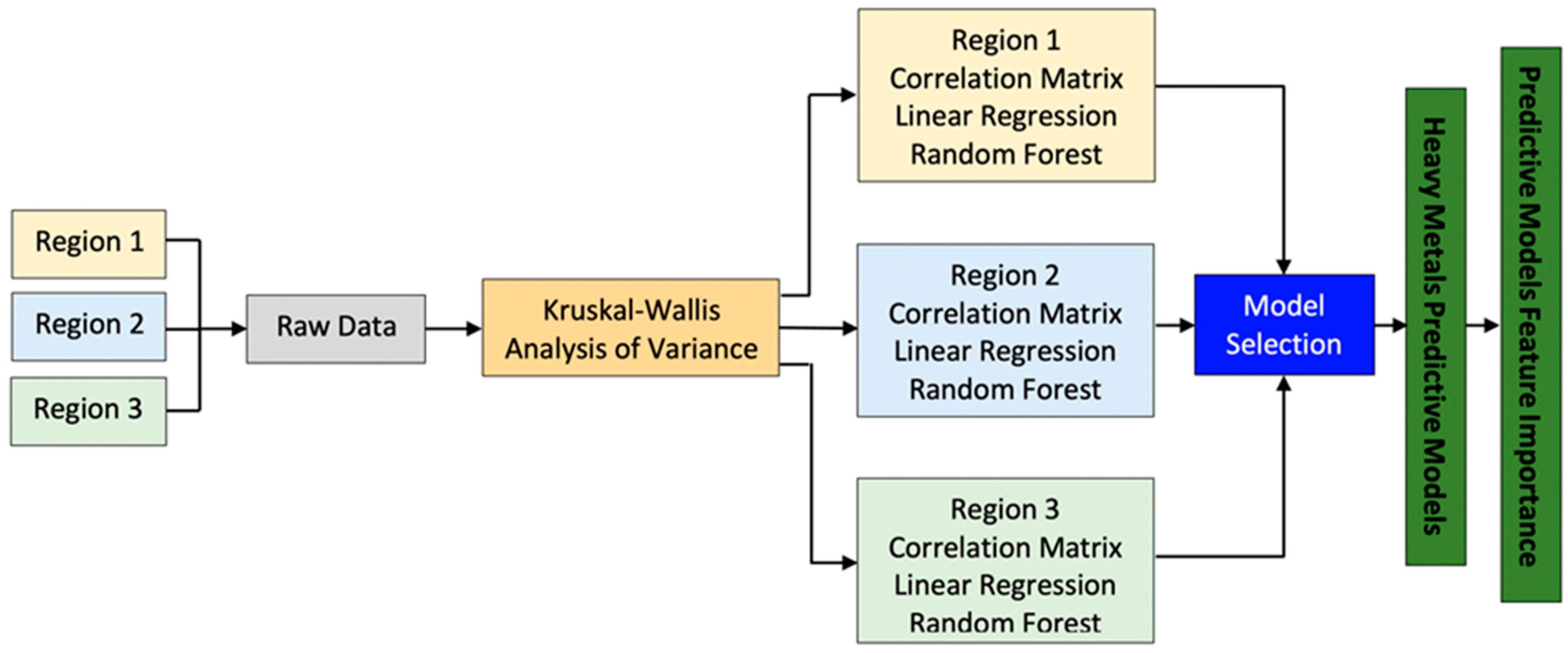
2.6. Model Development

In order to identify a predictive modelling framework for determining heavy metals concentration in fish hepatic and muscle tissues from LRDR, based on OS biomarkers, a series of procedures were performed, starting from the raw data and ending to final prediction models (Figure 2).
According to Figure 2, after collecting the raw data parameters from the three regions presented above, in order to understand if there are significant data differences between the regions, due to the non-normal distribution of the data, a Kruskal-Wallis analysis of variance was performed. The results indicated significant differences in regions data distribution, therefore each region was independently analyzed. A region analysis involved three main steps: (a) calculate the correlation matrix for acquiring the perspective over the existing linear relations in the dataset—with possible impact over the predictive techniques such as linear regression, retaining only the relevant values, respectively, above 0.6 and below −0.6; (b) develop linear regression models on normalized datasets (scaled regressors), using stepwise backward and forward selection for obtaining the most relevant predictors [58] and comparable coefficients that would help to distinguish between predictors relevancy; (c) develop predictive random forest models for the targeted features.
For choosing the final predictive models, the model selection procedure took into consideration two main metrics, respectively, R-Sq and Root Mean Square Error (RMSE). The R-sq has an intuitive scale as it ranges from zero to one, where zero indicates no improvement over the mean model, and one indicating perfect prediction having the entire dependent variable variance described by the predictors. The RMSE, the square root of the variance of the residuals, indicates the absolute fit of the model to the data. If R-sq is a relative measure of fit, RMSE is an absolute measure. RMSE is interpreted as the standard deviation of the unexplained variance, being in the same units as the response variable. RMSE is a good measure for describing how accurately a model predicts the response, being one of the most important fit criteria for predictive models based on OLS (ordinary least square) estimations [59].
Last step of the research procedure was to identify for each reliable predictive model the order of the most relevant predictors, being able this way to assess strong prediction influences of the various dependent variables. Regarding the predictive modelling procedure to determine the heavy metals concentration in fish liver and muscle tissues, the current research started with the multiple linear regressions, a technique that uses a number of explanatory variables to predict the outcome of the dependent variable, with the goal of modelling the linear relationship between the independent variables and the response variable. The following assumptions were tested: there is a linear relationship between the dependent variables and the independent variables, the predictors are not highly correlated with each other; yi observations are selected independently and randomly from the population; residuals should be normally distributed.
Due to the fact that for the existing context, all linear models poorly described the relations between predictors and dependent variables (low Adj-Rsq values), the current research needed to use a non-linear approach for obtaining reliable predictive models. Even if the MLR models explained a low to medium percentage of the dependent variable variance, the current research presents in Table A1 the MLR models for heavy metals prediction in both muscle and hepatic tissues as a reference for the subsequently RF models. There are many ways to handle non-linearity problems by using the current machine learning methodologies (e.g., polynomial regressions, artificial neural networks, tree-based regressors, ensemble learning, etc.).
When choosing one of these approaches, several factors should be considered: (a) volume of available data, (b) avoiding overfitting, (c) feature importance determination, (d) prediction accuracy, (e) data distribution
Measuring heavy metals concentration in muscle or liver tissue of the aquatic organic organisms is an expensive task in terms of time and financial resources. Thus, the volume of data cannot be expected to be large, therefore, any chosen prediction algorithm, should consider this aspect.
Random Forests (RF), the methodology used for the current research, handles well low volumes of data, performing optimal when a larger number of features are available.
RF represents an ensemble learning method [60]. That involves generating many classifiers/regressors, subsequently aggregating their results by using a boosting [61] or a bagging approach [62]. Boosting involves giving extra weight to points that were incorrectly predicted by earlier predictors, while for bagging, successive trees do not depend on earlier trees, being completely independent. The random forest approach offers an estimator that fits a number of decision trees on different subsamples of the dataset and uses averaging to control overfitting and to improve the predictive accuracy.
During the past six years, the random forest usage has steadily increased. By using Google Trends service, it was possible to collect historic data that was used to visualize the search interest for five prediction related terms: (a) linear regression—one of the most used prediction algorithms, (b) random forest, (c) XGBoost—a regularizing gradient boosting algorithm enforced by a strong community of data scientists [63], (d) CatBoost—one of the newest gradient boosting prediction algorithms [64], (e) prediction model—a generic term used to describe any of the previous mentioned algorithms (Figure 3).
As it can be observed in Figure 3, the search interest value for the ‘linear regression’ term is the highest (which is to be expected due to its age and worldwide popularity). However, both ‘random forest’ and ‘xgboost’ terms presents a consistent ascending trend in search popularity. On the other hand, from all the above algorithms, CatBoost is the newest one (released in 2017), hence it is not yet as popular as its counterparts.
In terms of comparison, it was possible, by using the collected data through the Google Trends service, to highlight country level differences for the above search terms. Thus, considering for each country all the above terms, their sum of search percentage value would be 100. For a visualization purpose, the search percentage value of each term for every country allowed several classes definition as follows: (a) six classes for linear regression term—class A with search percentages below 40%, class B with values between 40% and 50%, class C between 50–60%, class D between 60% and 70%, class E between 70% and 80%, class F above 80%, (b) four classes for random forest term—class A with search percentages below 10%, class B with values between 10% and 20%, class C between 20–30%, class D above 40%, (c) four classes for XGBoost term—class A with search percentages below 5%, class B with values between 5% and 10%, class C between 10–15%, class D above 15%, (d) four classes for CatBoost term—class A with search percentages below 2%, class B with values between 2% and 3%, class C between 3–4%, class D above 4%. For the linear regression term, the number of classes needed to be higher because the percentage values (of each country) were spread out on a larger interval.
Thus, clear differences related to the search interest in the above-mentioned search terms can be observed from the Figure A1, Figure A2, Figure A3 and Figure A4 between countries. If referring to linear regression term it can be noticed that the highest search interest percentage can be found in the USA, Canada, Australia, Norway or Finland and the lowest values in countries such as Russia, China, France or Spain. Switching to the remaining terms involving non-linear and more recent methodologies, it can be noticed that Europe and Russia display higher search interest percentage values.
Several papers [65,66,67,68] described the advantages of using random forest: (a) data normalization is not required, (b) reduced overfitting results, (c) works well with both continuous and categorical variables, (d) works well with a reduced number of samples; (e) data distribution is not relevant.
The RF predictions could be improved (if required) by adjusting several hyperparameters: the maximum depth of the trees), the number of trees in the forest of the model, the minimum number of samples required to be at a leaf node or the minimum number of samples required to split an internal leaf node.
In term of model validation, the prediction methodology used both the root mean square error (RMSE) and the R-square metrics for assessing model’s performance. All RF models were fitted using 80% of the data as training dataset. Thus, 20% of the data remained unseen to the models and could be used further on in the testing phase.
In addition to determining all reliable prediction models, another important aspect of the current research was to estimate the independent variables’ importance when predicting the dependent one. For linear regression model, it is quite easy to assess the predictors feature importance. For example, after performing feature scaling that would bring all values into the range (0,1), parameter coefficients could be compared to see which one has a higher impact for the overall prediction. Furthermore, for a linear model, the p-value metric could be used to determine the predictors’ importance in describing dependent parameter variance, being able to choose this way which one remains in the model. The random forest methodology offers also the possibility of assessing the importance of each predictor in predicting the dependent variable. For this, the ‘eli5’ Python library was used.
This library computes the parameter feature importance by measuring how the overall score decreases when a feature is not available. Thus, it is possible to rank the predictor variables in terms of relative significance, by calculating the decrease in node impurity weighted by the probability of reaching that node, probability that is calculated by the number of samples that reach the node, divided by the total number of samples [67,69,70,71]. When the value is high, the feature is more important.
n i j = w j C j w l e f t ( k ) C l e f t ( j ) w r i g h t ( j ) C r i g h t ( j )
where: nij represents the importance of node j; Cj = the impurity value of node j; left(j) = child node from left split on node j; right(j) = child node from right split on node j; wj = weighted number of samples reaching node j.
The importance for each feature on a decision tree is calculated according to the following formula:
f i i = j : n o d e   j   s p l i t s   o n   f e a t u r e   i n i j k a l l   n o d e s n i k
where: nij = the importance of node j; fii is the importance of feature i.
The values obtained from the above equation should be normalized (normfij) to values between 0 and 1 by dividing by the sum of all feature importance values:
n o r m f i i = j a l l   t r e e s n o r m f i i j T
The feature importance is the average over all the trees. The sum of the feature’s importance value on each tree is calculated and divided by the total number of trees:
R F f i i = j a l l   t r e e s n o r m f i i j T
where: T = total number of trees; normfiij = normalized feature importance for i in tree j; RFfii = the feature i importance, calculated from all the trees in the RF model.

3. Results and Discussion

3.1. Heavy Metals Data Analysis

Heavy metal concentration in the water samples collected from the Danube Delta and the Black Sea registered the following descendent trend: Fe > Cu > Zn > Pb > Cd, whereas in the Danube River the trend was Fe > Zn > Cu > Pb > Cd (Table 1). The highest values were recorded in the analyzed Danube River sector, followed by Black Sea Coast and Danube Delta (Table 1).
Several papers [24,72] emphasize the high exposure of the Danube River to pollution since it passes through many industrial zones and receives urban and industrial wastes, as well as agriculture leachate. Therefore, this can explain the high concentrations of heavy metals recorded in the Danube River sampling sector. In addition, the findings emphasize the capacity of Danube Delta to act as a buffer zone for pollutants transported by the Danube.
According to other studies [4,73], the Danube Delta is the largest wetland of the complex system pertaining to the Danube River and forms a complex network of river channels, bays, lakes, sandy banks and numerous marshes that contribute to improving the quality of the Black Sea water, acting as a buffer zone for pollutants in the Danube. Therefore, the analysis of heavy metals in samples collected from the studied aquatic macro-system confirms the existing connections between its components. Fe registers the highest concentration among all analyzed metals, situation which correlates with both technological processes applied in the Galați steel factory and Tulcea alumina refinery (Table 1). In addition, Zn records considerable high concentrations in all the sampling area, which can be due to shipyard activity, namely galvanization processes. The natural presence of metals in the lower sector of Danube River, generated by the bedrock erosion should be taken into consideration also. Depth erosion and vertical erosion is manifested especially in the upper sector of the river due to the presence of stones and gravel. In the middle sector, the riverbed is represented by grit and gravel and horizontal erosion is manifested. The lower sector of the river is characterized by sand and very fine gravel and horizontal erosion occurs also. In this sector, the river substrate is sand, frequently interspersed with mud, organic sludge, silt, loam and clay. In small percentages gravel is present in fine to medium size.
According to [74] the erosion in this area is moderate. The grain size along the Sf. Gheorghe branch has been previously characterized as fine to median sands and silts [75]. The authors concluded in their study that the highest levels of heavy metals in the Danube River sediments, between Bazias and flowing mouth in the Black Sea, are associated in the areas where mining activities are conducted (km 1049–km 995). As well, cluster and PCA analysis highlighted the fact that the concentrations of Cd, Cu, Pb and Zn in the branches of Danube River (Chilia, Sulina and Sf. Gheorghe) are influenced by anthropogenic activities, whereas Cr and Ni concentrations are influenced mainly by the presence of rocks naturally rich in these metals in the Romanian sector of Danube River [76].
The median iron concentration in rivers has been reported to be 700 µg/L [77]. However, the concentrations reported within the present study are significantly much higher. Hence, it can be stated that the bedrock of Danube River in the lower sector generates moderate concentrations of heavy metals and that abnormal high values are related to human activities. Similar results regarding Fe concentration in Danube River related to anthropogenic activities was previously reported in [54].
The data related to heavy metal concentration in water matrix are not considered proper to be included in the analytical framework prediction models since they could be highly variable among the Danube River basin during a short period of time, depending on a series of environmental factors such as water flow, water temperature, water level, occasional waste discharges.
Therefore, the data presented in Table 1 has the purpose of characterizing the environmental background of the analytical framework.
However, use of fish as bioindicators elaborating an analytical framework based on prediction models is more reliable since fish accumulate the metal concentrations during a longer time-period and due to their mobility, they can characterize a larger surface area.
The accumulation trend of heavy metals in the muscle tissue registered the following descending order: Fe > Zn > Cu > Cd > Pb in fish from Danube River, Danube Delta, respectively, and Fe > Zn > Cu > Pb > Cd in fish from the Black Sea (Table 2). In the case of the hepatic tissue, the accumulation tendency of heavy metals caught in the Danube River registered the same trend as for the muscle tissue (Table 2). Regarding the fish caught from the Danube Delta and the Black Sea, the accumulation trend of metals in the hepatic tissue was Fe > Zn > Cu > Pb > Cd, Fe > Zn > Cu > Cd > Pb (Table 2). Fe was the most abundant metal in both muscle and hepatic tissue. Nevertheless, the values registered for this element in the liver were at least 10 times higher compared to the values registered in the muscle. This fact is expected due to the liver’s implication in the synthesis of red blood cells [41]. The least abundant metals detected in the muscle and hepatic tissues were Cd and Pb. However, these elements can induce toxic effects on fish even in trace amounts. To avoid human intoxication with heavy metals due to fish consumption, the European legislation [78] sets a maximum permitted level of Cd (0.05 µg/g) and Pb (0.3 µg/g) concentration in fish muscle. In the entire studied macro-system, 25 of the total analyzed fish specimens registered values of Cd concentration in the muscle tissue above the maximum permitted level. In natural aquatic ecosystems, metals are not equally distributed, instead they accumulate in certain “hot spots”, influenced by hydraulics and water physico-chemical parameters. Thus, continuous monitoring of the water quality is needed to identify possible polluted sites.
By analyzing the differences between fish muscle tissue and fish hepatic tissue (Table 3), it can be observed that significant differences (p < 0.05) are recorded between DR and DD for heavy metal concentrations considered within this study. In addition, by comparing DR versus BS, it can be observed that Cd is the only metal which registered a statistically significant difference (p < 0.05). Furthermore, by comparing BS and DD, it was observed that Pb, Fe, Zn and Cu concentrations registered statistically significant differences (p < 0.05) (Table 3). In terms of heavy metals from the hepatic matrix, statistically significant differences (p < 0.05) were recorded for Pb, Cu and Fe between all the analyzed areas and, for Cd between DR and BS, respectively, DD and Zn between DD and DR, respectively, BS (Table 3).

3.2. Enzymatic and Non-Enzymatic Biomarkers Determination

All OS biomarkers register higher values in fish hepatic tissue matrix, compared to muscle tissue, except MDA in DD sampling area (Table 4). However, CAT, SOD and GPx registered the highest values in fish muscle tissues at DR, followed by DD and BS coast, while MDA records maximum values at DD, followed by BS coast and DR (Table 4). According to other studies [79] it can be stated that increased MDA levels are correlated to decreased SOD activity, under the context of heavy metals exposure. The SOD and MDA are the most sensitive OS biomarkers to metal exposure, followed by CAT and GPx. The hepatic matrix is first affected by pollution; thus, it can be used as a main indicator of environmental pollution occurrence. The highest values of SOD and GPx in hepatic matrix are recorded at DR, followed by DD and BS, while CAT registers the highest values in DR, followed by BS and DD (Table 4). This can be due to the fact that in the DR water, the highest values in case of the studied metals were registered, compared to DD and BS. The MDA hepatic values were in accordance with Cd values (Table 2) and revealed the highest concentrations in DD and DR (Table 4).
Significant differences (p < 0.05) are recorded between DD and DR, respectively, BS, when analyzing both fish muscle and fish hepatic tissue matrix in terms of all OS biomarkers considered in the present study (Table 5). However, not significant differences were recorded between DR and BS (p > 0.05) in terms of CAT, SOD, GPx and MDA, in both analyzed sample matrix (Table 5).

3.3. Pollution Index in the Analysed Area

The pollution index was calculated in order to better establish the experimental backgrounds for each study area. However, in order to calculate the pollution index, based on Romanian Regulation Order no. 161/2006 (Table 6), the study area was associated to a certain water quality class. According to the Romanian Regulation Order no. 161/2006, the quality class I is the best ranking, while quality class V is the worse. Thus, in terms of Cd concentration in water, both BS and DD are associated to I quality class, while DR is within the second class. Considering Pb, Zn and Cu, it can be stated that all analyzed area are associated to first water quality class. However, the Fe concentration places all analyzed areas in the fifth water quality class.
The pollution index points out a seriously affected aquatic environment by the presence of Fe in the entire macro-system Danube River-Danube Delta-Black Sea (Table 7). As well, Fe concentration in the water column is highly above the concentration specific to the quality class V for surface waters, mentioned in the Order 161/2006 by the Romanian Government (Table 6). In case of Zn accumulation in the water, a strongly affected aquatic environment was identified in the Danube River (Table 7). The presence of Fe and Zn in high concentrations is due to the intense naval activities conducted in the Lower sector of the river.
The values for the pollution index registered for the rest of the analyzed metals manifest no effect on the entire studied macro-system.

3.4. The Correlation Matrix

According to previous studies [3], the correlation matrix can be used as a tool to summarize the linear relationships existent in a dataset, as well as for identifying strong and relevant relationships that could be further modelled. In present study, all data related to heavy metals and OS biomarkers in both muscle tissue and hepatic tissue matrix were processed using Python NumPy library. According to other studies [80], weak positive and negative correlations would be considered in the range of 0.1 ÷ 0.3/−0.1 ÷ −0.3, moderate positive and negative correlation would range within 0.3 ÷ 0.5/0.3 ÷ 0.5, and strong positive and negative correlation between 0.5 ÷ 1.0/0.5 ÷ 1.0. However other studies which performed matrix correlation for heavy metals in different fish tissues considered as strong positive/negative all linear correlation with coefficient values over +0.7/−0.7. In addition, the correlation matrix is useful in analytical framework elaboration since in order to generate the prediction models, independent variables are supposed to be independent. According to similar studies [3], if the degree of correlation between variables is high enough, problems can arise when fitting the model and interpreting the results.
Positive significant correlations at BS are recorded within all OS biomarkers from both hepatic and muscle tissues (between 0.8–1). In addition, related heavy metals, Fe in muscle tissues is positively correlated with Cu (0.6) and Cd (0.6) in muscle, Fe (0.6), Cu (0.6) and Cd (0.7) in hepatic tissues. The Zn in muscle is positively correlated with Cd in both muscle and hepatic tissues (0.6) and negatively correlated with SOD (−0.6) in muscle and both CAT (−0.7) and GPx (−0.6) in hepatic tissue. In addition, Cd in muscle was found to be positively correlated with Cu (0.9) and Cd (0.9) in hepatic tissues, while Cu in muscle is strongly correlated with Cu (0.9) and Pb (0.7) in hepatic tissues.
In case of DD, positive significant correlations are recorded within all OS biomarkers from both hepatic and muscle tissues (between 0.7–0.9). In addition, related heavy metals concentration, the only strong positive correlation is observed between Zn in muscle and hepatic tissues (0.8). However, Pb in hepatic tissues is strongly correlated with CAT (0.7), SOD (0.8), GPx (0.7) and MDA (0.7) in hepatic tissues.
The correlation matrix revealed positive correlations between Cu in muscle and Cu (0.9), Pb (0.7) and Cd (0.9) in hepatic tissues, as well as Cd in muscle tissues (0.9). Some studies have emphasized that Cu enters the fish body mainly via food [81,82]. At the level of the intestine epithelium, Cu is transferred in the blood stream and then transported to the liver, due to its implication in organism detoxification. The presence of Cu in the liver is also related to the natural protein binding such as metallothioneins [83]. Even more, besides its storage purpose, the liver acts as a redistributor of metals to other organs, such as the muscle [83]. This phenomenon could stand as a possible explanation for the positive correlation registered between the Cu concentration in fish liver and fish muscle. This fact was confirmed in [84], where the authors highlighted a positive correlation in the concentration of Pb between the liver and muscle tissues. As well, the positive correlation between Cu and Cd in fish tissue (gonads) was previously observed in [85] in Alosa braschinkowi. Nevertheless, the correlation between metals in the fish body is highly dependent on the physiological processes within the organism, the presence of other metals and interactions between them [3].
In addition, Cd in muscle tissues is positively correlated with Cu (0.9), Pb (0.6) and Cd (0.9) in hepatic tissues, while Cd in hepatic tissue correlates positively with Cu (0.9) and Pb (0.6) determined from the same hepatic tissues. However, the Fe in hepatic tissue is the only elements which strongly correlate, positively, with OS biomarkers, more precisely, with MDA from hepatic tissues (0.8).

3.5. The Multi Linear Regression (MLR) Models

In order to generate predictive models between heavy metals and OS biomarkers from both hepatic and muscle tissues matrix, MLR was used. Therefore, the resulted equations are presented in Table A1. However, from a total of 29 MLR models, only 2 models record good performance. Both models help predicting the Fe in hepatic tissues, at BS and DR area, and explain 88.00%, respectively, 88.80% of the variance of this parameter. Therefore, the most important independent variable for the prediction of Fe concentration in hepatic fish tissues at both BS and DR are MDA, followed by CAT and SOD from hepatic tissue (Table A1).
It can be observed that MLR methods do not offer a substantial feed-back in order to elaborate an analytical framework aimed to predict the heavy metals concentration in fish tissues, based on OS biomarkers. In the literature, MLR were found useful for predicting micro-elements, based on macro-elements in fish tissues [3]. In addition, other authors manage to apply MLR for predicting elements in soil and crops [86], different water bodies [87] or different aquatic animals as mollusks [88].
Therefore, since MLR did not perform as expected, in order to accomplish the aim of this present study, RF based models were applied.

3.6. Non-Linear Models, Based on Random Forest (RF) Algorithm

According to other studies [3], non-linear models are tested for determining possible models among the parameters that did not register linear correlation between each other. Therefore, in the present study, after applying the RF technique on all the dataset, a number of 30 RF models were identified (Table 8), 10 models for each of the studied region (BS coast, DD and DR), all with high prediction accuracy (Figure A5, Figure A6, Figure A7, Figure A8, Figure A9, Figure A10, Figure A11, Figure A12, Figure A13, Figure A14, Figure A15, Figure A16, Figure A17, Figure A18, Figure A19, Figure A20, Figure A21, Figure A22, Figure A23, Figure A24, Figure A25, Figure A26, Figure A27, Figure A28, Figure A29, Figure A30, Figure A31, Figure A32, Figure A33 and Figure A34). The weight of all independent variables was identified after running the feature importance algorithm in order to determine the importance of a specific OS biomarker parameter in determining the heavy metal dependent variable value (Table 8).
The RF models for BS coast revealed that the prediction of Cd concentration in hepatic tissues is mostly based on MDA and CAT in hepatic tissues, while Cd in muscle tissues is influenced by GPX in both muscle and hepatic tissues and MDA in hepatic tissues. The prediction of Pb in hepatic tissues is significantly depended by MDA and GPx from hepatic tissues and SOD from muscle tissues, respectively, while Pb prediction in muscle tissues is mostly dependent by GPX in both hepatic and muscle tissues. The prediction of Fe in hepatic tissues depends on MDA and GPx from hepatic tissue, while Fe in muscle tissue is mostly dependent on GPx in hepatic tissues and CAT in muscle tissues. For Zn prediction in hepatic tissue, SOD hepatic and MDA muscle and hepatic are most significant independent parameters that must be considered, while for Zn prediction in muscle tissues, CAT hepatic and both GPX, hepatic and muscle, must be considered as most important. The Cu prediction in both muscle and hepatic tissues emphasizes MDA hepatic and SOD muscle, respectively, CAT muscle as most important parameters.
The analysis of RF models registered based on DD database revealed that Cd concentration in hepatic tissues is mostly based on CAT and SOD in muscle tissues, while Cd in muscle tissues is influenced by CAT and GPX in muscle, respectively, MDA in hepatic tissues. The prediction of Pb in hepatic tissues is significantly depended by MDA and CAT from hepatic tissues, while Pb prediction in muscle tissues is mostly dependent by GPX and MDA in muscle tissues. The prediction of Fe in hepatic tissues depends on CAT and GPx from muscle tissue, while Fe in muscle tissue is mostly dependent on SOD and GPx in hepatic tissues. For Zn prediction in hepatic tissue, CAT and SOD in muscle are most significant independent parameters that must be considered, while for Zn prediction in muscle tissues, both GPX and CAT in hepatic tissues must be considered as most important. The Cu prediction in both muscle and hepatic tissues emphasizes MDA and CAT in hepatic tissues, respectively, CAT in muscle and GPX in hepatic tissues as most important parameters.
The analyzed database from DR region reveals that Cd concentration in hepatic tissues is mostly based on MDA in muscle tissues, followed by GPx and SOD in hepatic tissues, while Cd in muscle tissues is influenced by MDA in both analyzed tissues. The prediction of Pb in hepatic tissues is significantly depended by MDA and GPx from muscle tissues, while Pb prediction in muscle tissues is mostly dependent by GPX in muscle tissues and CAT in hepatic tissues. The prediction of Fe in hepatic tissues depends on MDA from both analyzed tissues, while Fe in muscle tissue is mostly dependent MDA and CAT in hepatic tissues. For both Zn predictions in hepatic and muscle tissues, the MDA in both in muscle and hepatic tissues are most significant independent parameters that must be considered. The Cu prediction in hepatic tissues emphasizes MDA, followed by SOD, CAT and GPx in hepatic tissues as most important parameters, while Cu in muscle can be mostly predicted by considering MDA in both analyzed tissues.
Random forest represents a good alternative to linear regression when the observed phenomenon is not linear. It produces reliable results, works well on both small and large datasets and it also creates estimates in case of missing data. Still, one of the major challenges comes from the fact that, at times, random forests are not able to extrapolate well over previously unseen data. The value in the leaves is calculated as an average of n observations. This approach improves the algorithm’s accuracy, reduce the over-fitting, but it can lead to the extrapolation issue, where the predicted values (for previously unseen data) will not be outside the training set values for the target variable. This issue can be minimized by increasing the number of samples in the training dataset, allowing the algorithm to train on a wider data interval. For the current research context, as the number of samples in the dataset is not high, the extrapolation problem could lower the accuracy of the RF models. However, by adding new data to the dataset, after performing new analysis, would mitigate this issue. The Danube River Basin Management Plan (DRBMP) targets the monitoring of the following metals: silver, bismuth, arsenic, cadmium, cobalt, chromium, copper, manganese, nickel, lead, rubidium, antimony, selenium, tin, thallium, uranium, vanadium, tungsten and zinc. The present study can support DRBMP through the effective prediction of metals in the muscle tissue, based on the prediction metrics performance. Therefore, 3 categories of heavy metals can be identified as it follows: 1st category (R-sq between 70.00–80.00%) includes only Cu, 2nd category (R-sq between 80.00–90.00%) includes Zn and Pb, 3rd category (R-sq between 90.00–100.00%) includes Cd and Zn. Therefore, in order to quantify the importance of OS biomarkers for predicting the heavy metals concentration in both fish muscle and hepatic tissues, weight level of each predictor was evaluated and presented in Table 9.
The analysis revealed in Table 9 emphasizes that MDA in hepatic tissue is the most important independent variable for predicting heavy metals in fish muscle and tissues at BS coast, followed by GPx in both hepatic and muscle tissues. The RF analytical framework revealed that CAT in muscle tissue, respectively, MDA and GPx in hepatic tissues are most common predictors for determining the heavy metals concentration in both muscle and hepatic tissues, in DD area (Table 9). For DR, MDA in muscle, followed by MDA in hepatic tissue are the main predictors in RF analysis (Table 9).
The presence of environmental pollutants can generate increased OS in fish and the main enzymes that mitigate the negative effects of this process are SOD, CAT and GPx. The SOD triggers ROS destruction by catalyzing the dismutation of O2 into H2O2, which CAT and GPx further reduces into H2O and O2 [21]. The GPx is the most important peroxidase and holds the essential role for erythrocyte protection against H2O2. The antioxidant defense system can be more intense in the liver, due to the occurrence of several oxidative reactions and ROS generation in this organ. Ratn et al. [89] revealed in their study a positive correlation between SOD and CAT activity in the liver of Channa punctatus and Zn bioaccumulation in the same organ. According to the pollution index calculated in this study, the concentration of Zn strongly affects the aquatic ecosystems of Danube River and, thus, induced OS to the resident biota. Table 10 presents centralized data related to OS biomarkers in different fish species and heavy metals in water/liver samples, according to different studies. Mohanty with co-authors [21] reported in their study a more intense activity of SOD and CAT in the muscle, specifically hepatic (SOD between 2–3 U/mg protein, respectively, 12 U/mg protein; CAT between 100–150 nkat mg protein, respectively, between 10,000–15,000 nkat/mg protein) tissues of Notopterus notopterus specimen collected from a polluted site of the Mahanadi river, in India, compared to a specimen collected from a non-polluted site. This phenomenon is also confirmed in the present study through higher enzymatic activity in the tissues of fish collected from Danube River, which is a seriously affected aquatic environment, according to the pollution index.
In addition, [35] pointed out in their study that the exposure of the common carp to Cd significantly increased the levels of MDA in the liver tissue (Table 10). Hajirezaee et al. [38] registered increased MDA level in the plasma collected from Mugil cephalus individuals exposed to Pb compared to the ones in the control group. This is similar to our results, since the sampled tissues from fish collected from Danube Delta registered the highest MDA levels and Cd concentration in the muscle of these fish was above the maximum permitted level by the EU regulation. The MDA represents the end-product of lipid peroxidation degradation and high levels indicate oxidative cell damage after toxicant exposure. In the study by [33], Cyprinus carpio individuals were exposed, for one week, to a mixture of metal pollutants (Cu: 4.8 μg/L; Cd: 2.9 μg/L and Zn: 206.8 μg/L). The authors registered no sign of OS in the liver and the gill tissues during that period. However, the decreased enzymatic activity of CAT and GPx under long-term metal exposure can lead to the manifestation of OS in the fish organism. It is difficult to define a narrow range for OS biomarkers in fish from the natural environment, because the concentrations of heavy metals are dynamic and the organism adapts its metabolism accordingly, by either increasing or decreasing the involved enzymes and antioxidants.
It is well known that aquatic organisms can be used as sentinels for an assessment of environmental contamination assessment by toxic chemicals, especially through the importance of ROS in physiological processes and toxicity mechanisms [79]. It is well known that heavy metals will accumulate in the fish liver tissue, compared to the muscle, due to the liver involvement in organism detoxification [4]. Increased metal levels in the liver generate a decreased SOD activity and increased lipid peroxidation [72]. Fish inhabiting water environments rich in Cd show increased generation of ROS, because Cd competes with essential metals for protein-binding sites, and thus, triggers the release of Fe2+ and Cu2+ ions [91]. In addition, in their study, [92] highlighted that oxidative stress caused by cadmium lead to cell death in trout hepatocytes. One mechanism of cellular injury in animals and indicator of oxidative stress in cells is lipid peroxidation [79]. An indicator of lipid peroxidation is malondialdehyde (MDA) and increased levels of MDA are associated to a variety of chronic diseases in vertebrates [79]. In their study, [79] highlighted a positive correlation (R2 f = 0.966 and 0.987) between Cd and Pb concentrations in fish plasma and muscle, and the MDA levels in the same matrix. In addition, the author noted that increased MDA levels are correlated to decreased SOD activity, within the context of heavy metal exposure. [93] registered in their study elevated MDA levels in the liver of catfish exposed to Zn, Cu, Pb, Cd and As, which is attributed to the livers affinity to accumulate the aforementioned metals. Thus, metals are catalyzers in ROS formation. Further, high levels of SOD in the liver are a response to oxidative stress caused by the presence of heavy metals, which generated the production of superoxide anions which activated SOD to convert the superoxide radical to H2O2 [93]. In case of CAT, a decreased activity compared to the rest of the antioxidant enzymes is expected due to inhibition by the wave of superoxide radicals [94,95,96]. The decreased CAT activity may be due to the flux of superoxide radicals, which have been shown to inhibit CAT activity [93]. Li with co-authors [97] demonstrated in their study that lipid peroxidation is enhanced in animals exposed to Cd compared to animals exposed to Zn.
Similar to most of the studies, the design of the current study is subject to limitations. Therefore, the analytical framework from present study was entirely based on fish muscle and hepatic tissues heavy metals and OS biomarkers. However, in future studies, water quality parameters data are recommended to be integrated in order to create a more precise and complex analytical framework, since it is well known that water hardness, alkalinity and pH influence the uptake process of potentially toxic metals by fish [55] and metals as Cd and Pb are bioavailable for fish to absorb if the aforementioned factors are low. Data from a wider study area should be collected, for several scenarios, in order for testing different approaches requiring larger data volumes such as neural network/deep learning or support vector regression. Furthermore, the ensemble modelling techniques function similar to a black box, meaning it can provide excellent predictive models, but difficult to interpret in terms of existing relation among predictors or between predictors and the dependent variable. Thus, more interpretable models could be used, such as for example the General Additive Models (GAM) which are generalized linear models, having the response variable depending on various smooth functions applied to predictors [98].

4. Conclusions

The present study points out the pollution of DR with Fe and Zn, due to intensive naval activities conducted in the lower sector of the river. In DD, Cd is present in the fish muscles in concentrations above the maximum level permitted by the EU regulations, due to the intensive agricultural activities conducted in the area.
The resident fish from DR manifest OS, through the highest activity of biomarkers CAT, SOD and GPx in muscle and liver tissues, compared to fish from DD and BS. The fish from DD, registered the highest values for MDA level, compared to the rest of the studied aquatic ecosystems.
The use of machine learning, through random forest algorithms, for the prediction of Cd, Pb, Zn, Fe, Cu in fish muscle and liver has proven to be an effective, fast and cost- effective tool for monitoring pollution in DR, DD and BS.
This study revealed, for each analyzed region, the most important parameters used for the heavy metals’ prediction. Thus, for the Black Sea coast, the MDA in hepatic tissue was identified as the most important independent variable for predicting heavy metals in fish muscle and tissues, followed by GPx in both hepatic and muscle tissues. For the Danube Delta, the random forest models revealed that CAT in muscle tissue, respectively, MDA and GPx in hepatic tissues were the most important predictors and for the remaining Danube regions, the MDA in muscle, followed by the MDA in hepatic tissue were the main predictors for the RF analysis.
Using the biomarker MDA from fish tissue to predict heavy metal concentrations in fish muscle can replace time-consuming and expensive field and laboratory analysis. In addition, it can help detect areas susceptible to pollution and it can identify contaminated fish with heavy metals in the Danube River Basin.

Author Contributions

Conceptualization, I.-A.S., D.S.C. and Ș.-M.P.; methodology, A.M.; software, D.S.C. and Ș.-M.P.; validation, M.M.T.R. and V.C.; formal analysis, R.J.; investigation, E.C.; resources, M.N.; data curation, R.J.; writing—original draft preparation, I.-A.S., D.S.C. and Ș.-M.P. All authors have read and agreed to the published version of the manuscript.

Funding

This work was supported by a grant of the Romanian National Authority for Scientific Research and Innovation, CNCS/CCCDI—UEFISCDI, project PN-III-P2-2.1-PTE-2019-0697, within PNCDI III.

Institutional Review Board Statement

This article does not contain any studies with human participants or laboratory animals performed by any of the authors. The fish were legally purchased.

Informed Consent Statement

Not applicable.

Data Availability Statement

Not applicable.

Acknowledgments

In the loving memory of our colleague Stefan-Adrian STRUNGARU, who prematurely passed away on 9 April 2021, thank you for the support and helpful discussion in writing this research article. The work of Simionov Ira-Adeline was supported by the project “ANTREPRENORDOC”, Contract no. 36355/23.05.2019, financed by The Human Capital Operational Programme 2014–2020 (POCU), Romania. This paper was supported by the project CNFIS-FDI-2021-0443. Active measures to increase and streamline the capacity for research, development, innovation and technology transfer at the “Dunărea de Jos” University of Galați—CEREX-UDJG_2021.

Conflicts of Interest

The authors declare no conflict of interest. The funders had no role in the design of the study; in the collection, analyses or interpretation of data; in the writing of the manuscript or in the decision to publish the results.

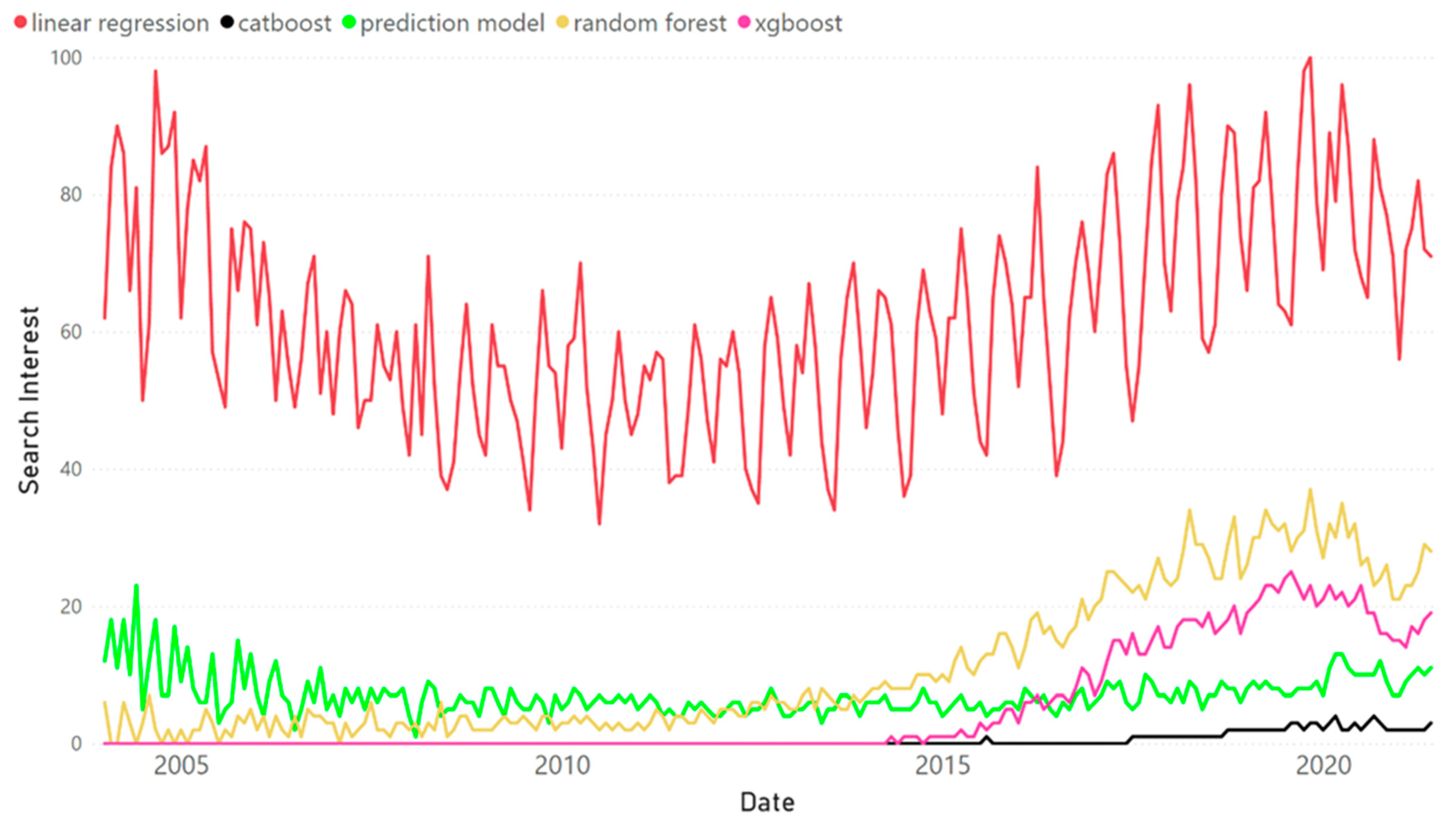
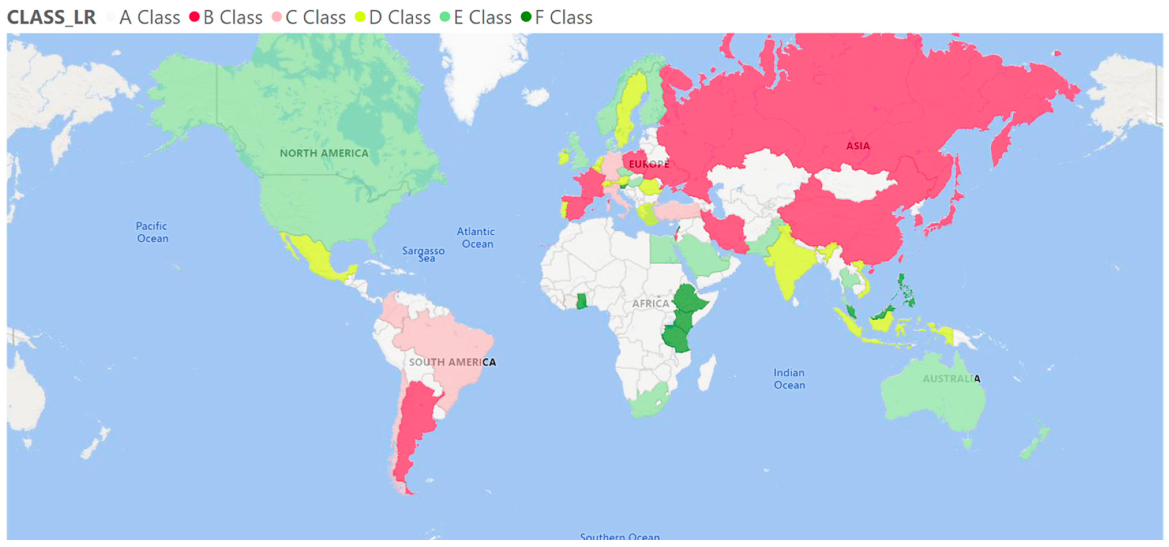
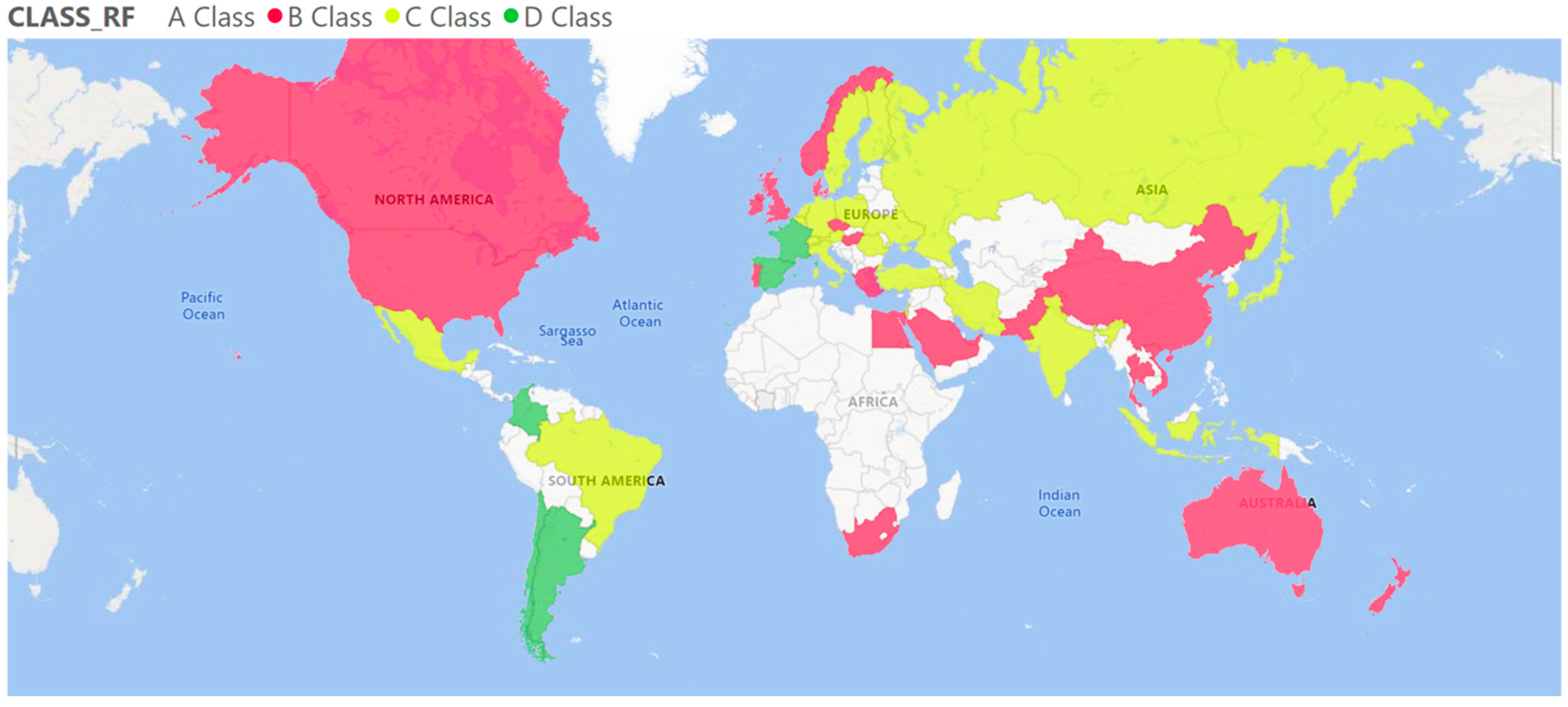
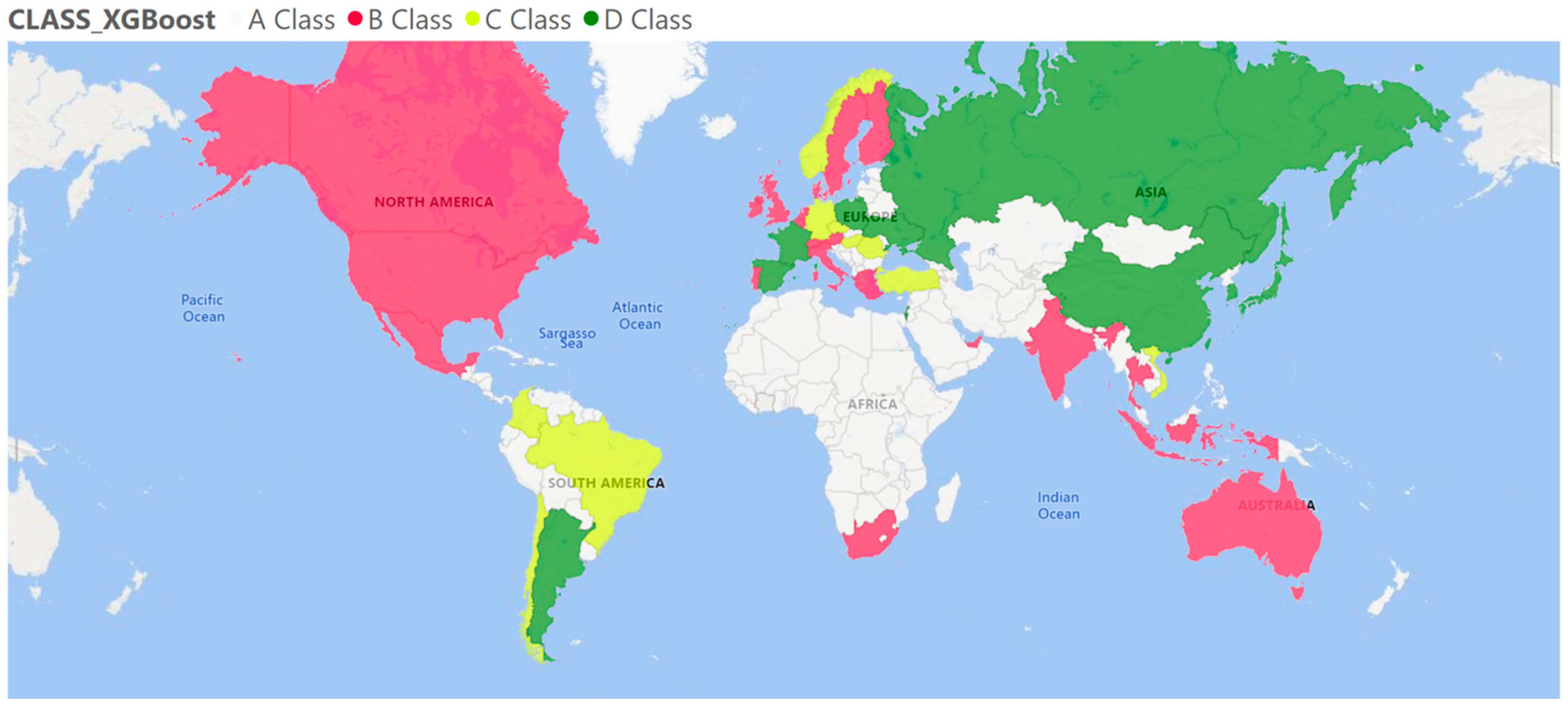
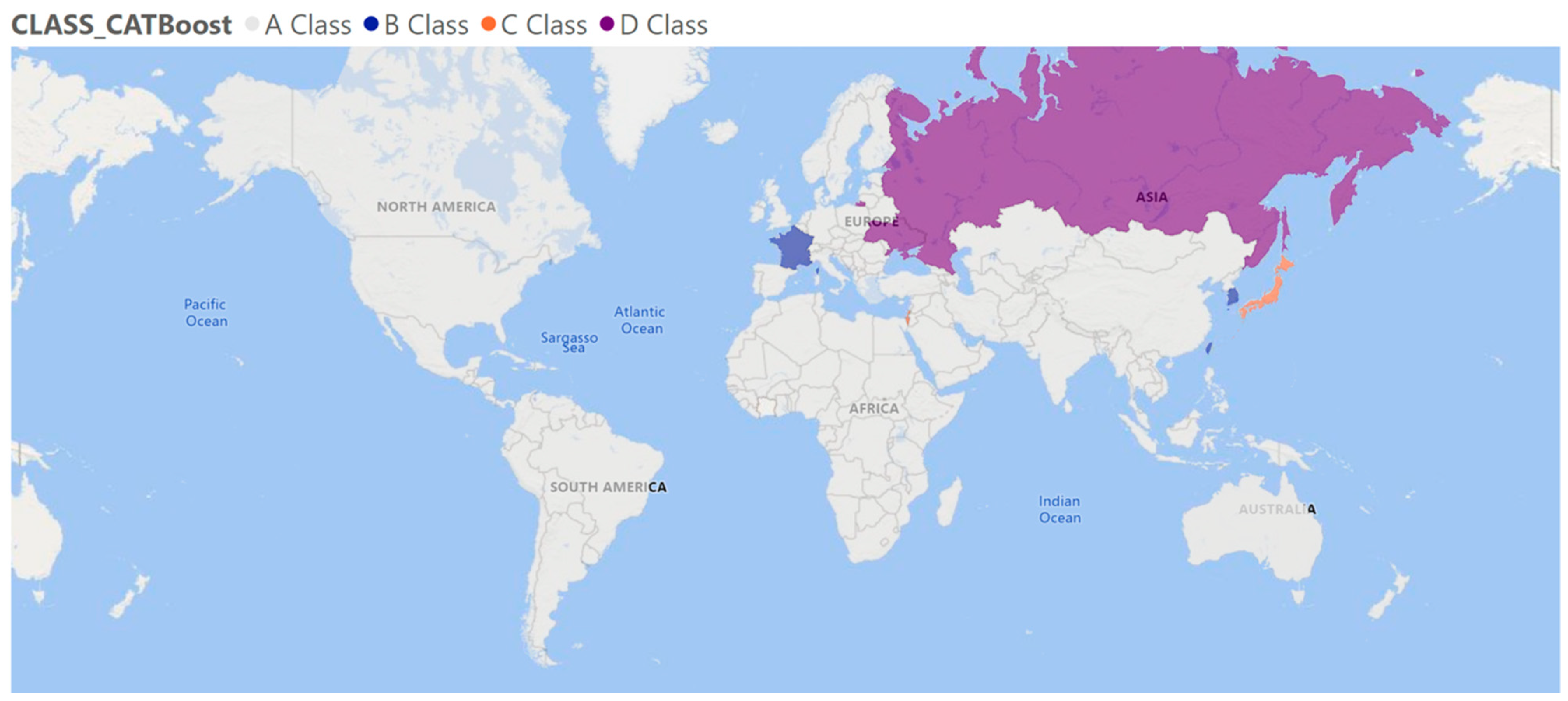
Appendix A. Worldwide Distribution of the Keyword Search Percentage

Figure A1. Worldwide term search distribution for ‘linear regression’ (data source: Google Trends Analytics).
Sustainability 13 08936 g0a1
Figure A2. Worldwide term search distribution for ‘random forest’ (data source: Google Trends Analytics).
Sustainability 13 08936 g0a2
Figure A3. Worldwide term search distribution for ‘linear regression’ (data source: Google Trends Analytics).
Sustainability 13 08936 g0a3
Figure A4. Worldwide term search distribution for ‘linear regression’ (data source: Google Trends Analytics).
Sustainability 13 08936 g0a4

Appendix B. The MLR Models for Heavy Metals Prediction

Table A1. The MLR models for heavy metals prediction in both muscle and hepatic tissues.
Dependent VariablePredictorsMLR EquationR-sq.
BS Coast
Zn muscle GPx muscle, CAT hepaticZn muscle = 0.590 + 0.423 GPx muscle − 0.924 CAT hepatic48.00%
Zn hepatic CAT muscle, MDA muscle, CAT hepatic, SOD hepaticZn hepatic = 0.507 + 0.401 CAT muscle − 0.379 MDA muscle − 1.092 CAT hepatic + 0.926 SOD hepatic37.49%
Fe muscle GPx muscle, CAT hepatic, SOD hepaticFe muscle = 0.375 − 0.919 GPx muscle − 1.097 CAT hepatic + 2.067 SOD hepatic43.00%
Fe hepatic CAT muscle, SOD muscle, CAT hepatic, SOD hepatic, MDA hepaticFe hepatic = 0.043 + 0.397 CAT muscle − 0.705 SOD muscle − 0.939 CAT hepatic + 0.929 SOD hepatic + 1.072 MDA hepatic88.00%
Cd muscle CAT muscle, CAT hepatic, SOD hepatic, GPx hepaticCd muscle = 0.007 + 0.945 CAT muscle − 1.058 CAT hepatic + 1.321 SOD hepatic − 0.985 GPx hepatic46.24%
Cd hepatic CAT muscle, CAT hepatic, SOD hepatic, GPx hepaticCd hepatic = 0.085 + 0.843 CAT muscle − 1.019 CAT hepatic + 1.419 SOD hepatic − 1.127 GPx hepatic48.15%
Pb muscle CAT muscle, MDA hepaticPb muscle = 0.045 + 0.186 CAT muscle + 0.209 MDA hepatic29.19%
Pb hepaticCAT muscle, CAT hepatic, SOD hepatic, GPx hepaticPb hepatic = 0.243 + 0.631 CAT muscle − 0.776 CAT hepatic + 1.190 SOD hepatic − 1.006 GPx hepatic41.68%
Cu muscleCAT muscle, CAT hepatic, SOD hepatic, GPx hepaticCu muscle = −0.001 + 0.871 CAT muscle − 0.701 CAT hepatic + 1.413 SOD hepatic − 1.335 GPx hepatic59.13%
Cu hepatic CAT muscle, CAT hepatic, SOD hepstic, Cu hepatic = 0.002 + 0.913 CAT muscle − 1.055 CAT hepatic + 1.531 SOD hepatic − 1.257 GPX hepatic54.94%
DD
Zn muscle CAT muscle, SOD muscle, GPx muscle, GPx hepaticZn muscle = 0.393 + 0.532 CAT muscle + 0.536 SOD muscle − 0.405 GPx muscle − 0.708 GPx hepatic44.84%
Zn hepatic CAT muscle, SOD muscle, GPx muscle, CAT hepaticZn hepatic = 0.224 + 0.471 CAT muscle + 0.497 SOD muscle − 0.422 GPx muscle − 0.457 CAT hepatic46.72%
Fe muscle SOD hepaticFe muscle = 0.168 + 0.288 SOD hepatic11.71%
Fe hepatic SOD muscle, GPx muscle, MDA hepaticFe hepatic = 0.743 − 0.759 SOD muscle − 0.554 GPx muscle + 0.691 MDA hepatic52.41%
Cd muscle CAT muscle, SOD muscle, MDA hepaticCd muscle = −0.039 + 0.554 CAT muscle − 0.446 SOD muscle + 0.340 MDA hepatic37.32%
Cd hepatic CAT muscle, MDA hepaticCd hepatic = 0.007 + 0.449 CAT muscle − 0.199 MDA hepatic23.62%
Pb muscle ---
Pb hepaticSOD muscle, SOD hepaticPb hepatic = 0.393 − 0.170 SOD muscle − 0.327 SOD hepatic59.87%
Cu muscleSOD hepaticCu muscle = 0.172 + 0.324 SOD hepatic13.87%
Cu hepatic SOD muscle, MDA hepaticCu hepatic − 0.424 + 0.571 SOD muscle − 0.732 MDA hepatic31.24%
DR
Zn muscle CAT in hepatic tissue and GPx in muscle tissueZn muscle = 0.589 − 0.924 CAT hepatic + 0.423 GPx muscle48.00%
Zn hepatic CAT hepatic, SOD hepatic, CAT muscle, MDA muscleZn hepatic = 0.507 − 1.092 CAT hepatic − 0.926 SOD hepatioc + 0.401 CAT muscle − 0.379 MDA muscle37.49%
Fe muscle CAT hepatic, SOD hepatic, GPx muscleFe muscle = 0.375 − 1.097 CAT hepatic + 2.067 SOD hepatic − 0.919 GPx muscle43.00%
Fe hepatic CAT hepatic, SOD hepatic, MDA hepatic, CAT muscle, SOD muscleFe hepatic = 0.024 − 0.717 CAT hepatic + 0.937 SOD hepatic + 1.221 MDA hepatic + 0.433 CAT muscle − 0.688 SOD muscle88.80%
Cd muscle CAT hepatic, SOD hepatic, GPx hepatic, CAT muscleCd muscle = 0.007 − 1.058 CAT hepatic + 1.321 SOD hepatic − 0.985 GPx hepatic + 0.945 CAT muscle46.24%
Cd hepatic CAT hepatic, SOD hepatic, GPx hepatic, CAT muscleCd hepatic = 0.085 − 1.019 CAT hepatic + 1.419 SOD hepatic − 1.127 GPx hepatic + 0.843 CAT muscle48.15%
Pb muscle MDA hepatic, CAT musclePb muscle = 0.045 + 0.209 MDA hepatic + 0.186 CAT muscle25.74%
Pb hepaticCAT hepatic, SOD hepatic, GPx hepatic, CAT musclePb hepatic = 0.243 − 0.776 CAT hepatic + 1.190 SOD hepatic +GPx hepatic + 0.631 CAT muscle41.68%
Cu muscleCAT hepatic, SOD hepatic, GPx hepatic, CAT muscleCu muscle = −0.001 − 0.701 CAT hepatic + 1.413 SOD hepatic − 1.335 GPx hepatic + 0.871 CAT muscle59.13%
Cu hepatic CAT hepatic, SOD hepatic, GPx hepatic, CAT muscleCu hepatic = 0.002 − 1.055 CAT hepatic + 1.531 SPD hepatic − 1.257 GPx hepatic + 0.913 CAT muscle54.94%

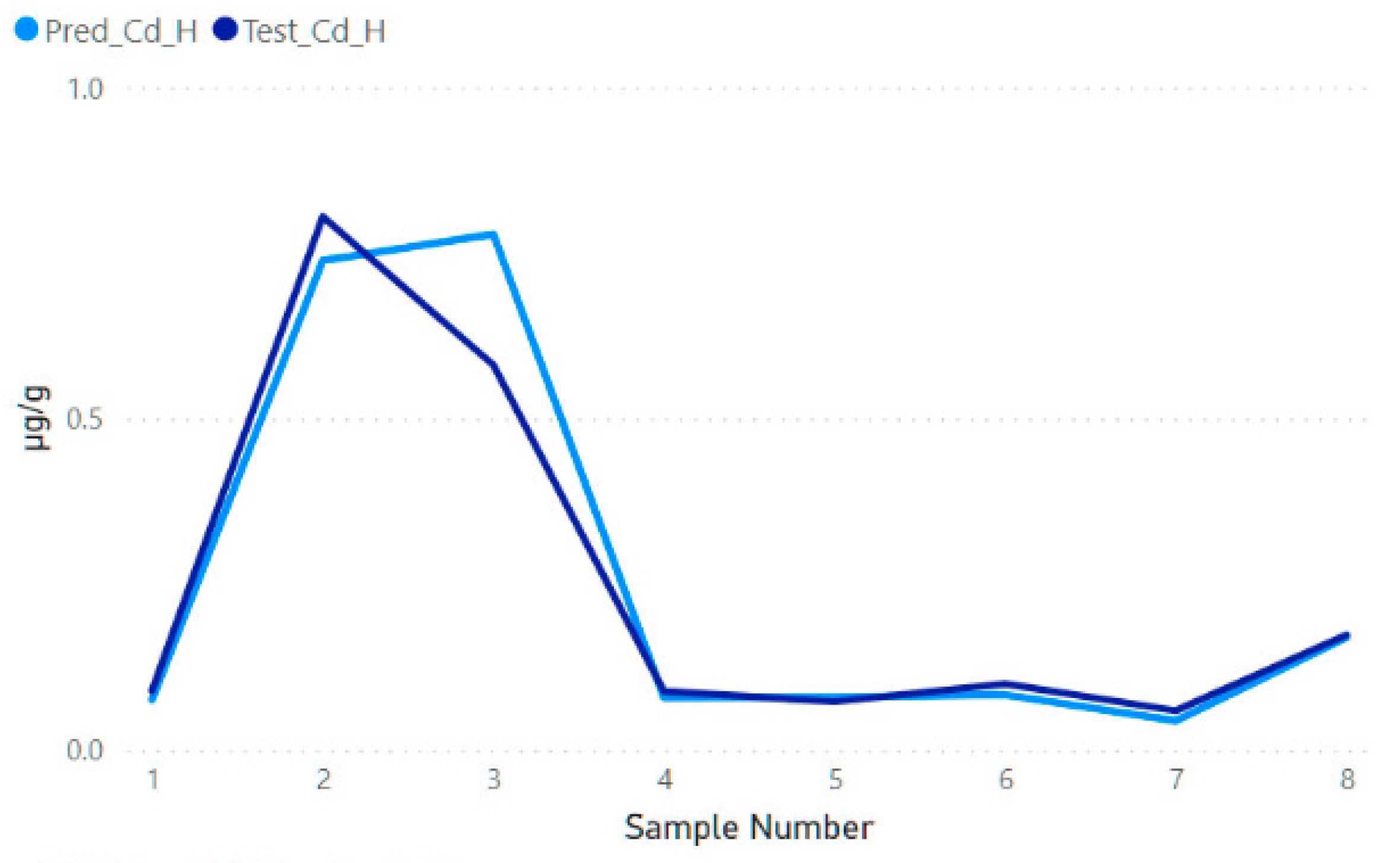
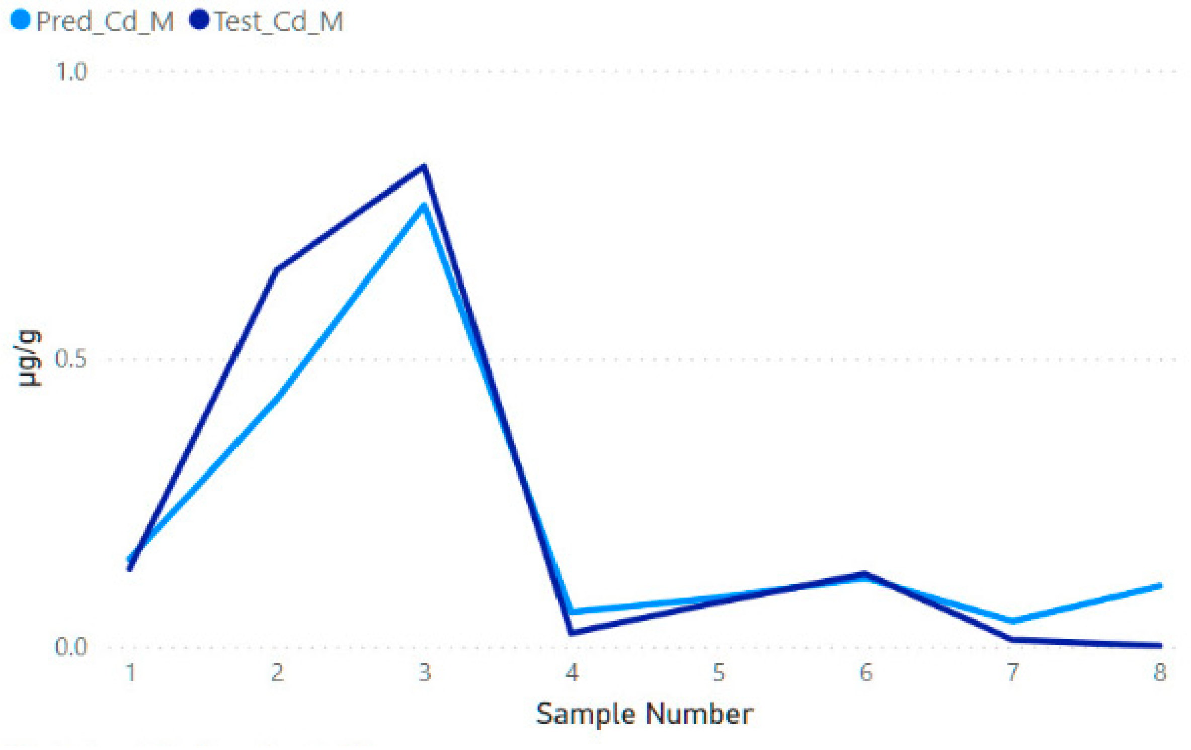
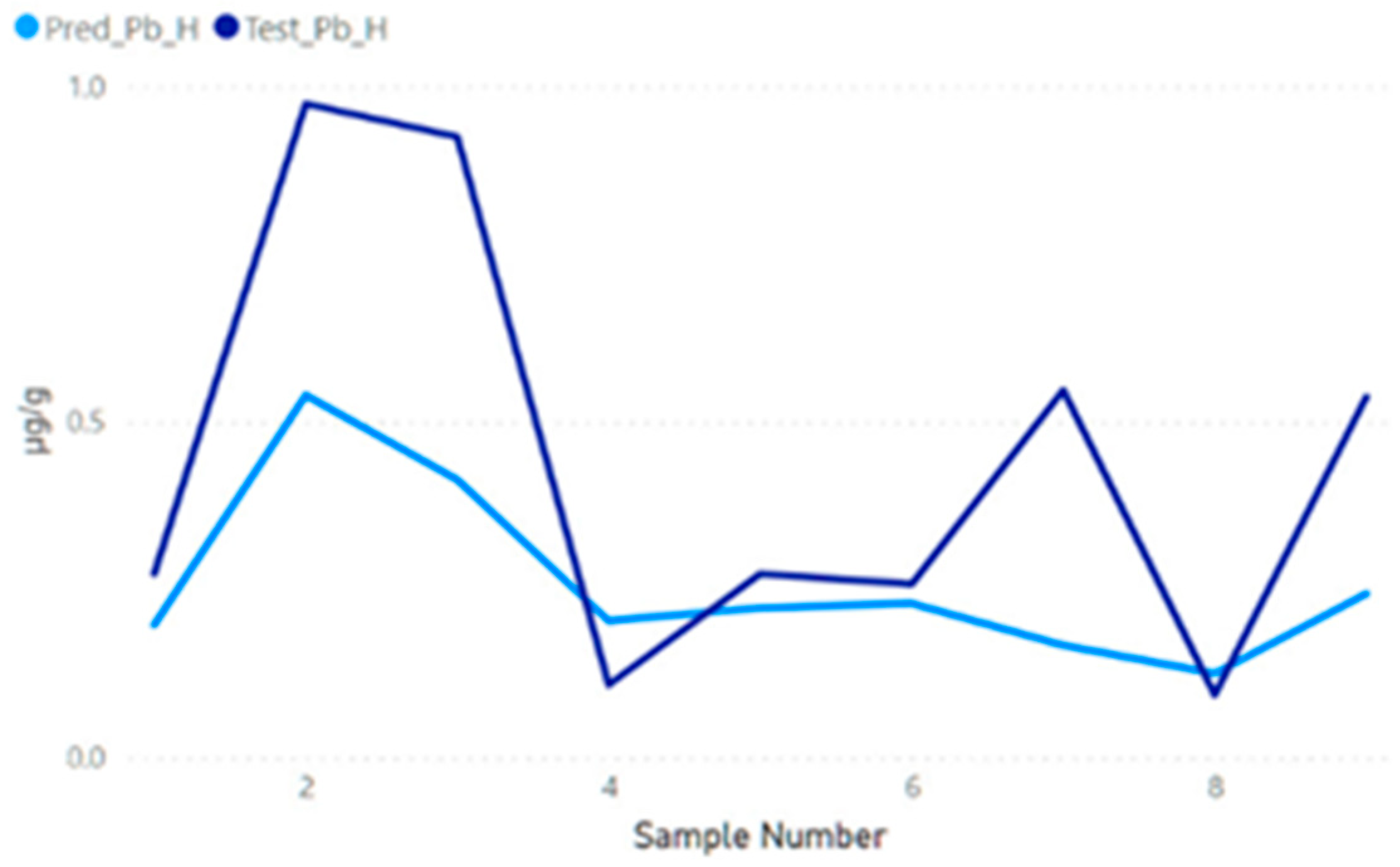
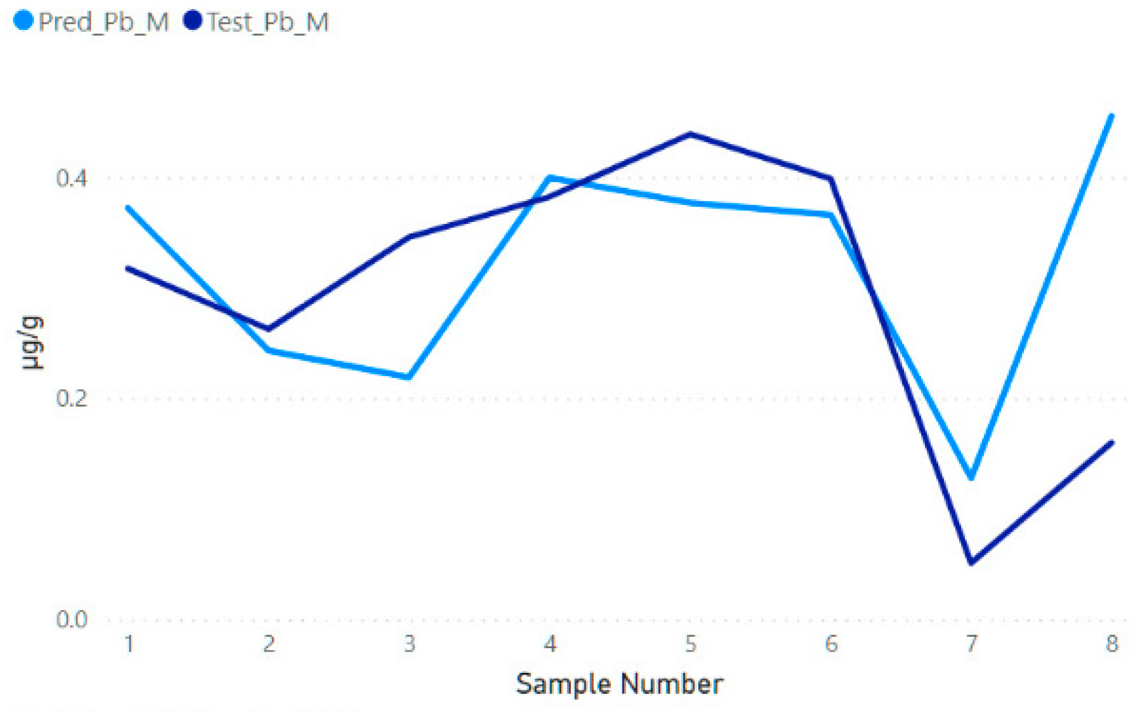
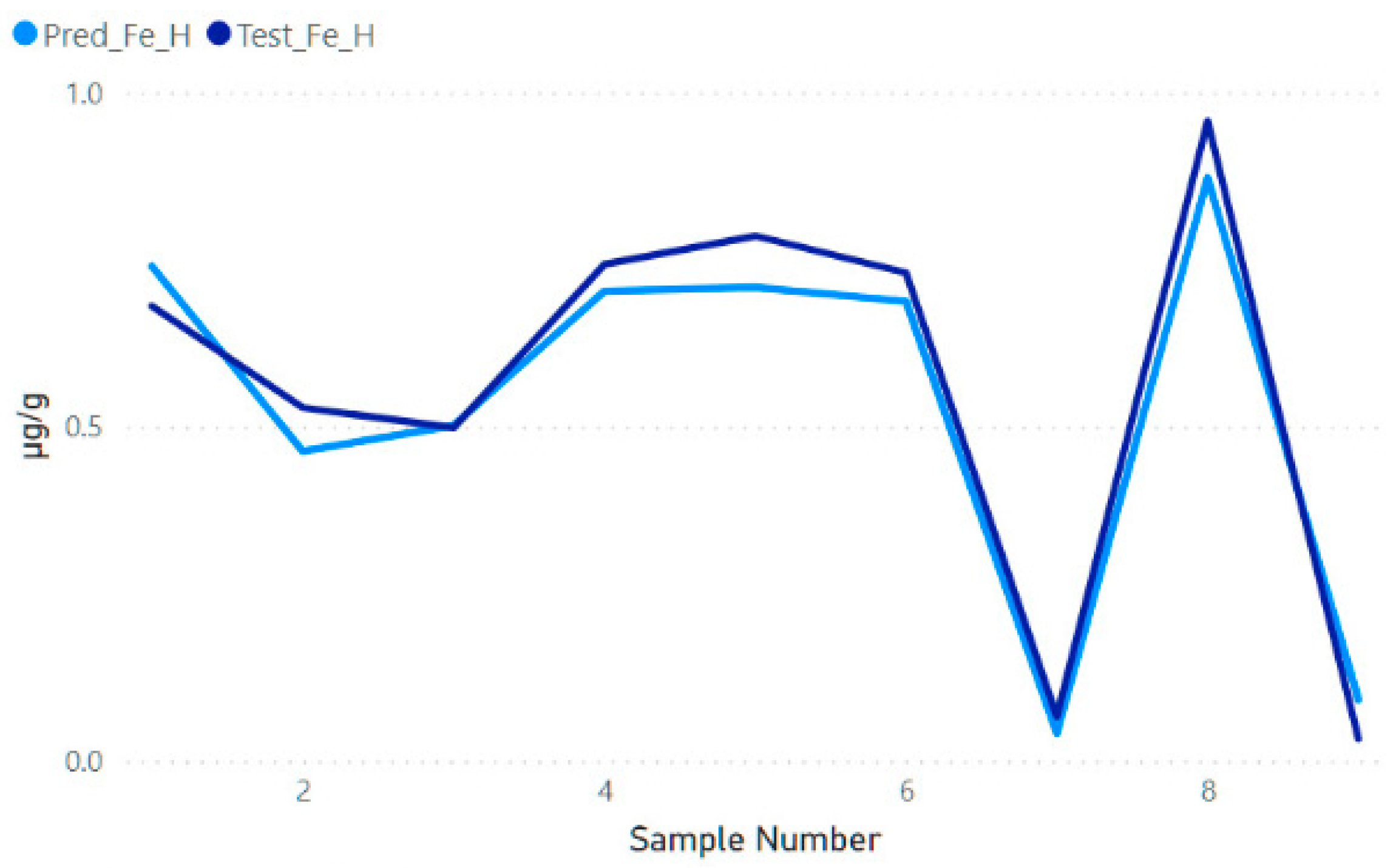
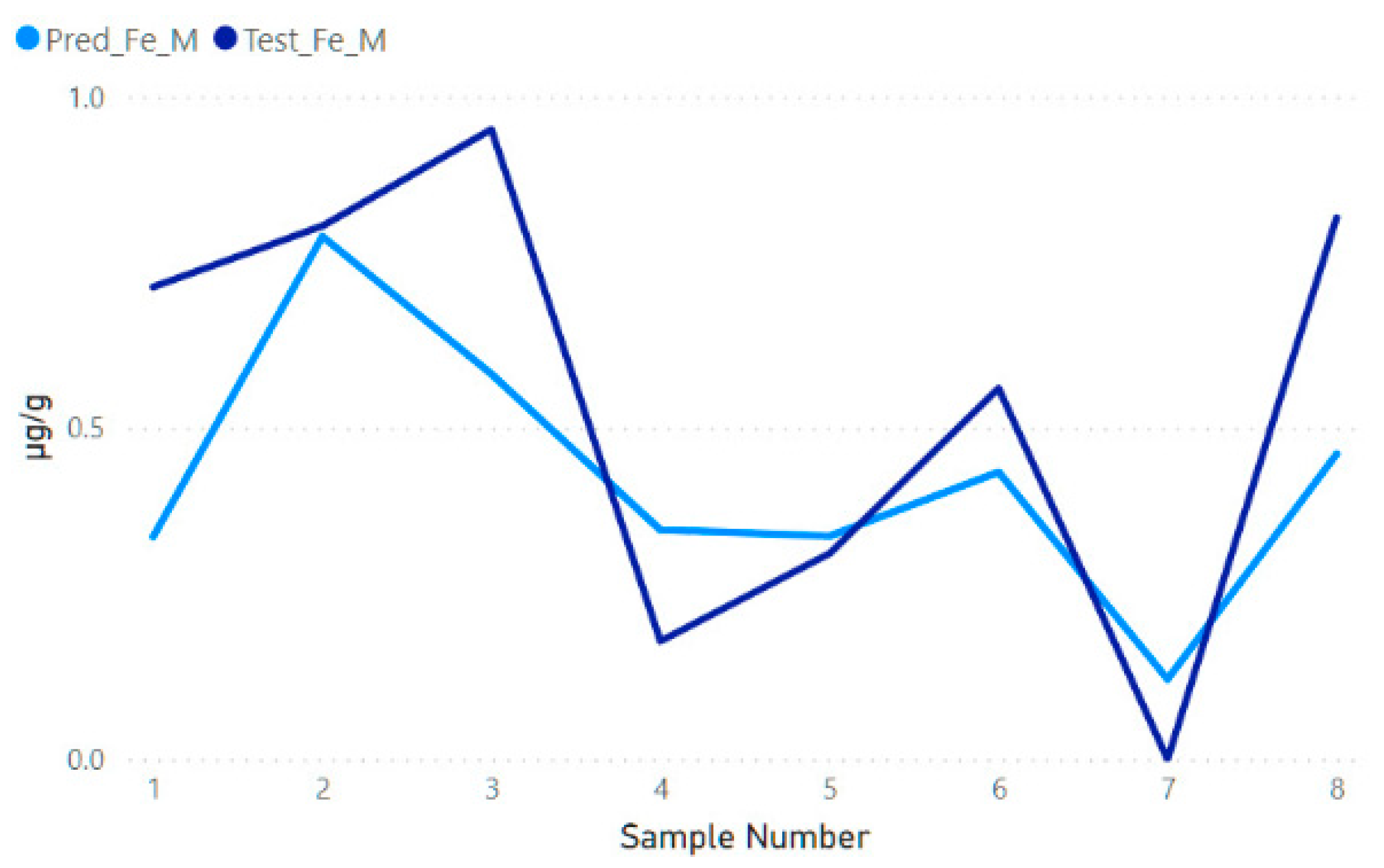
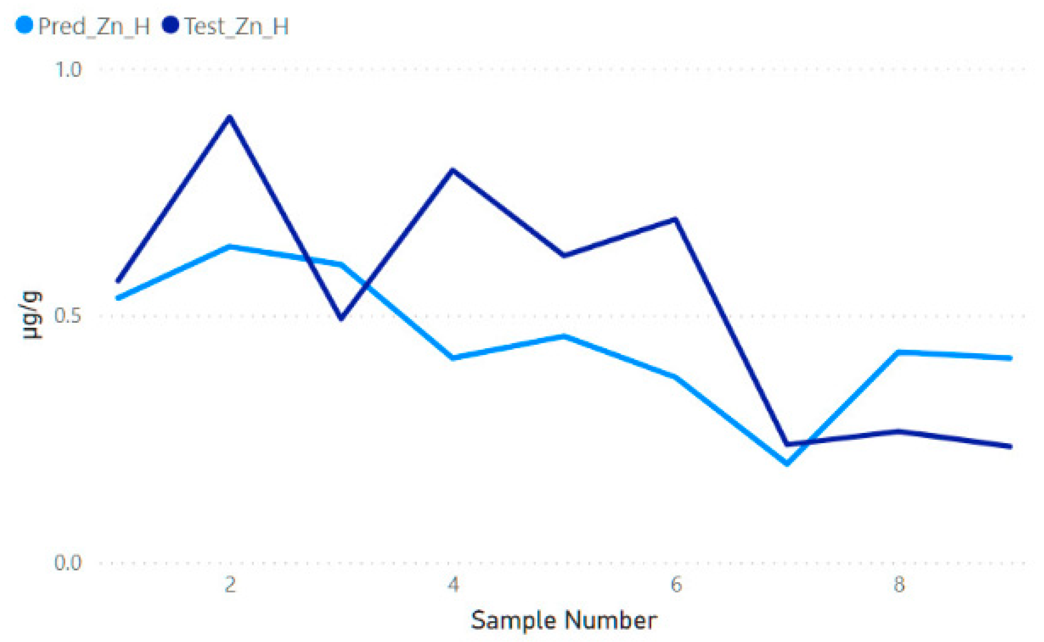
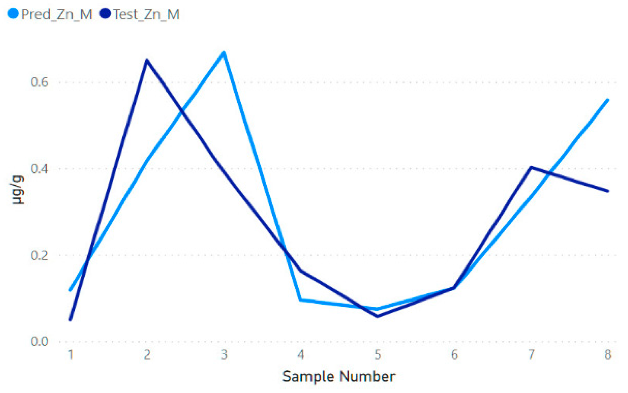
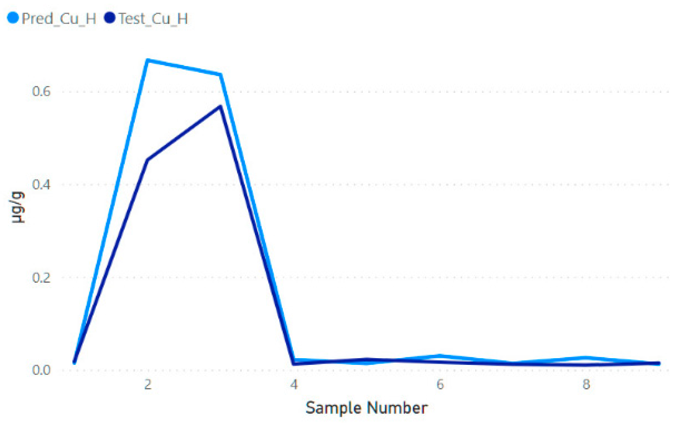
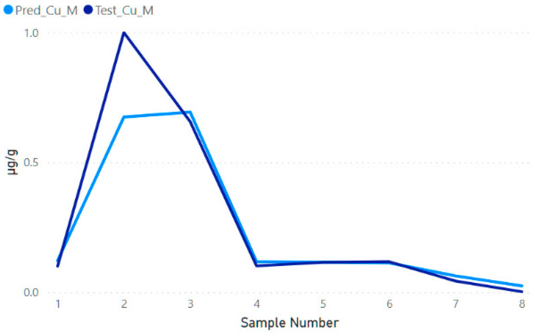
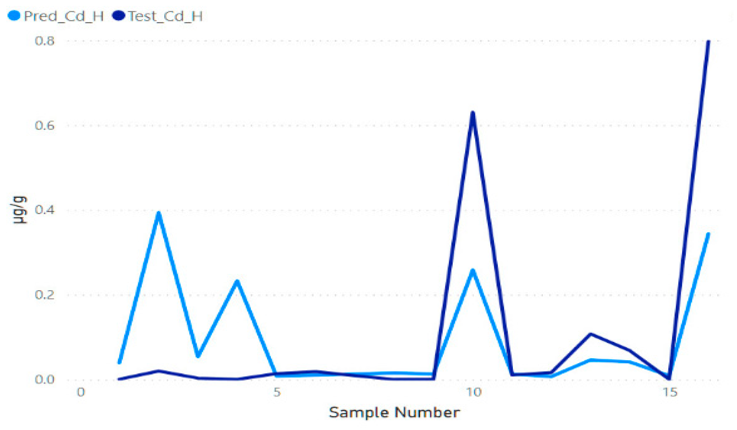
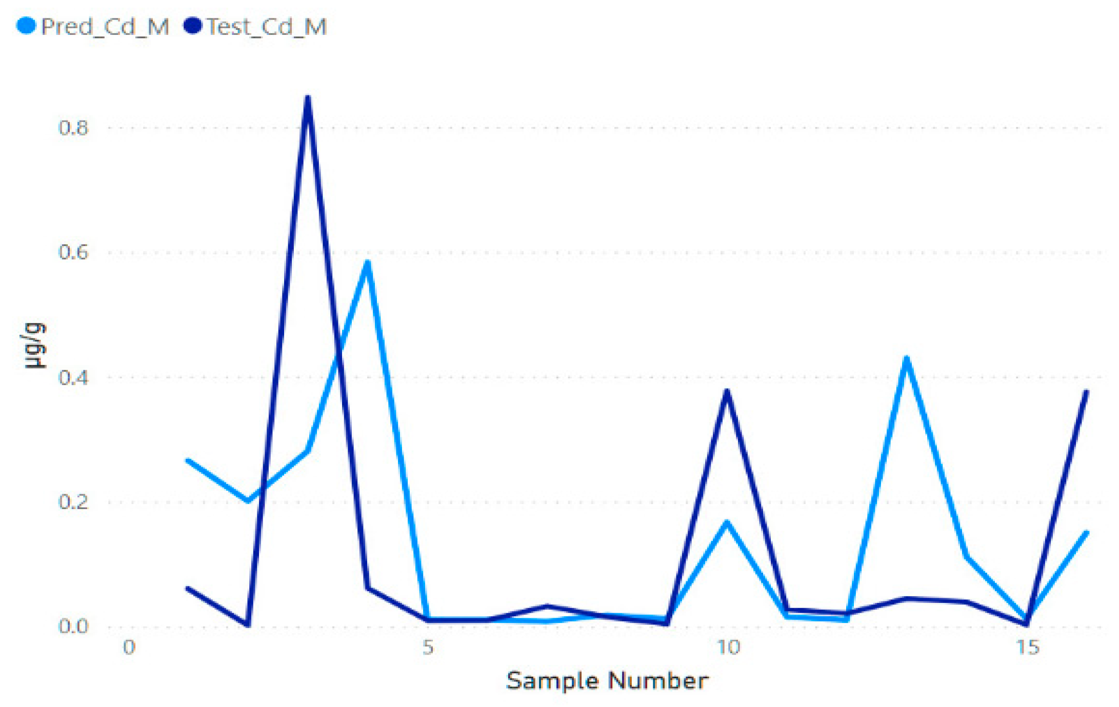
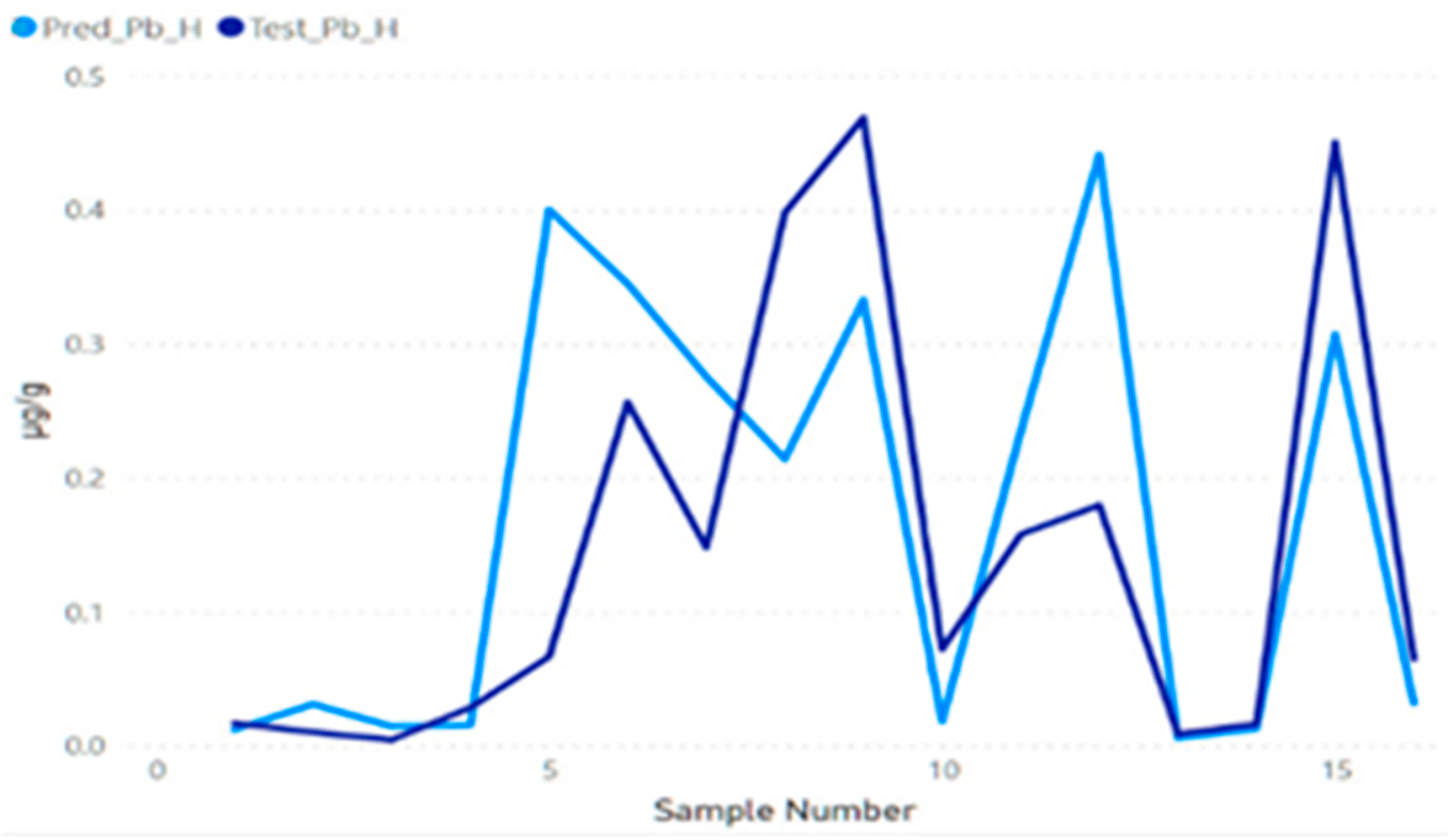
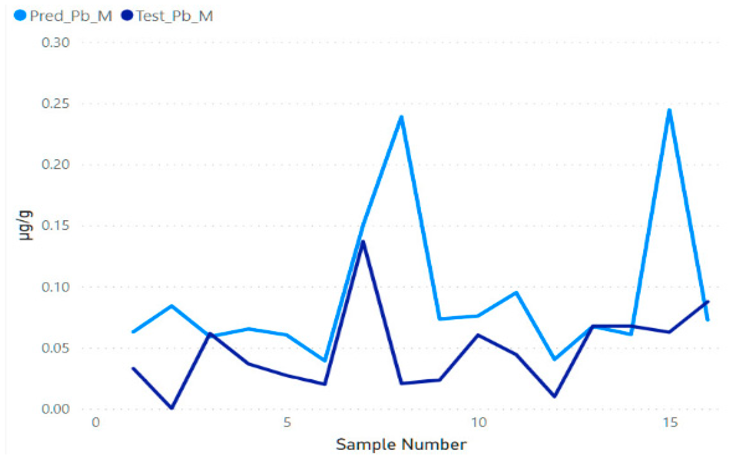
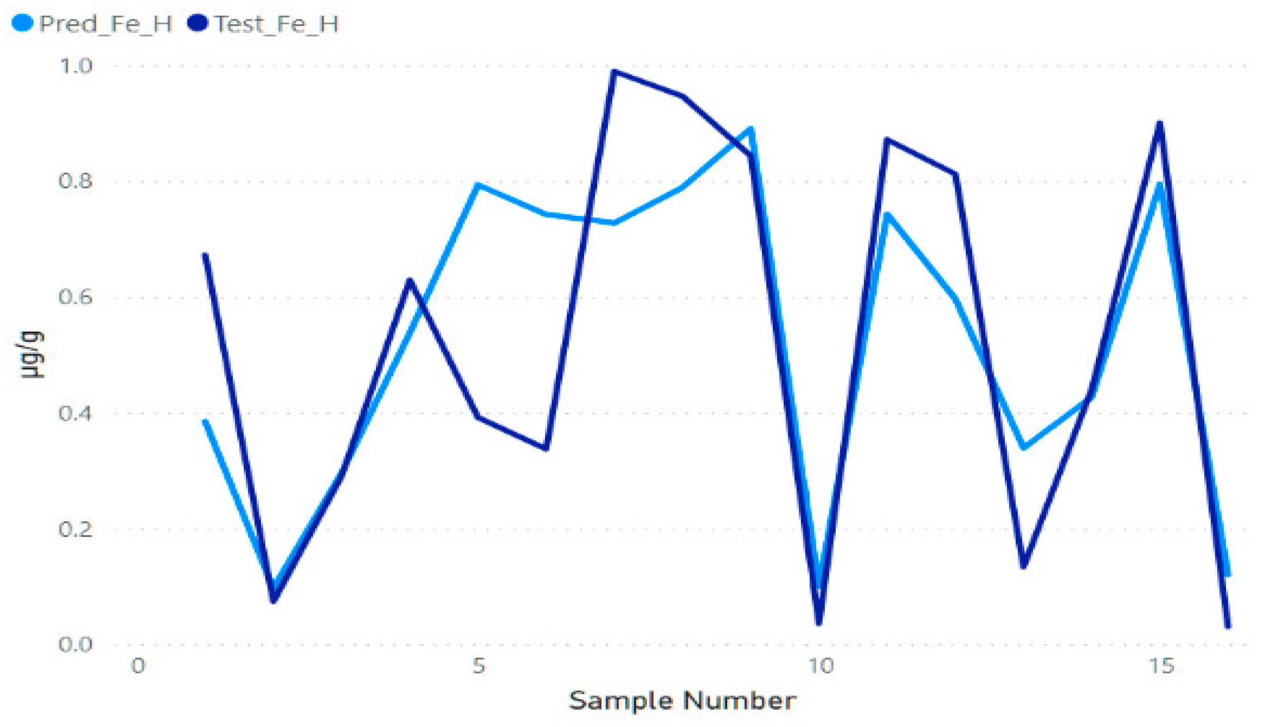
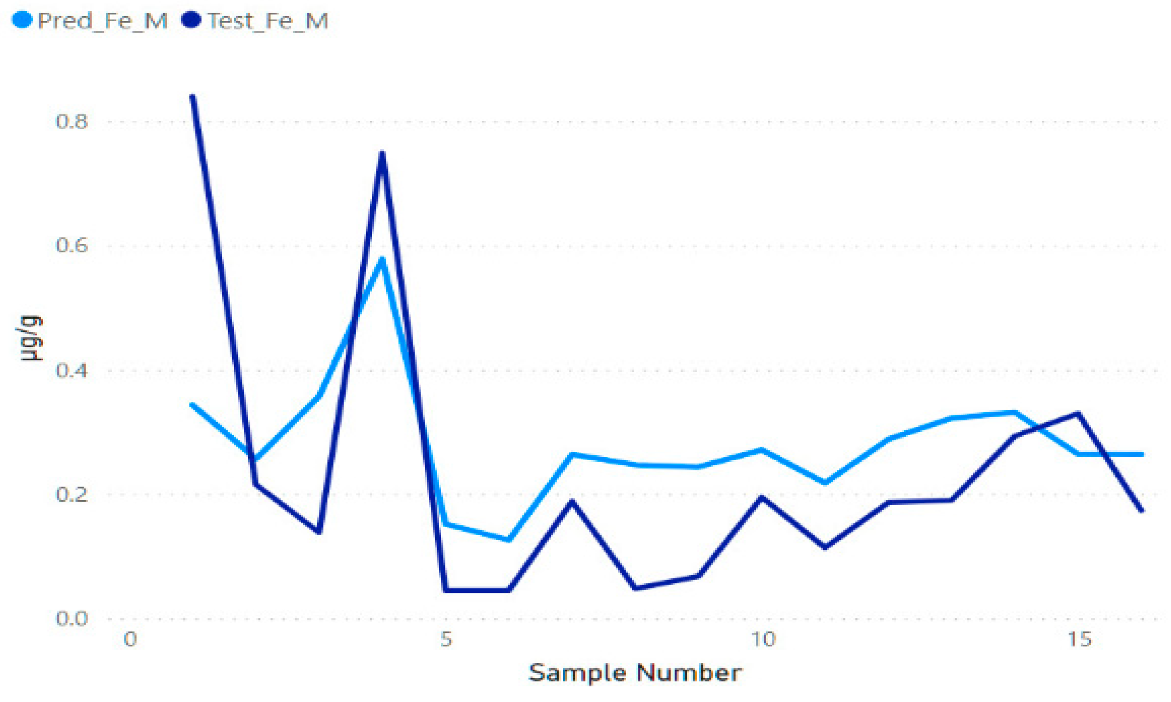
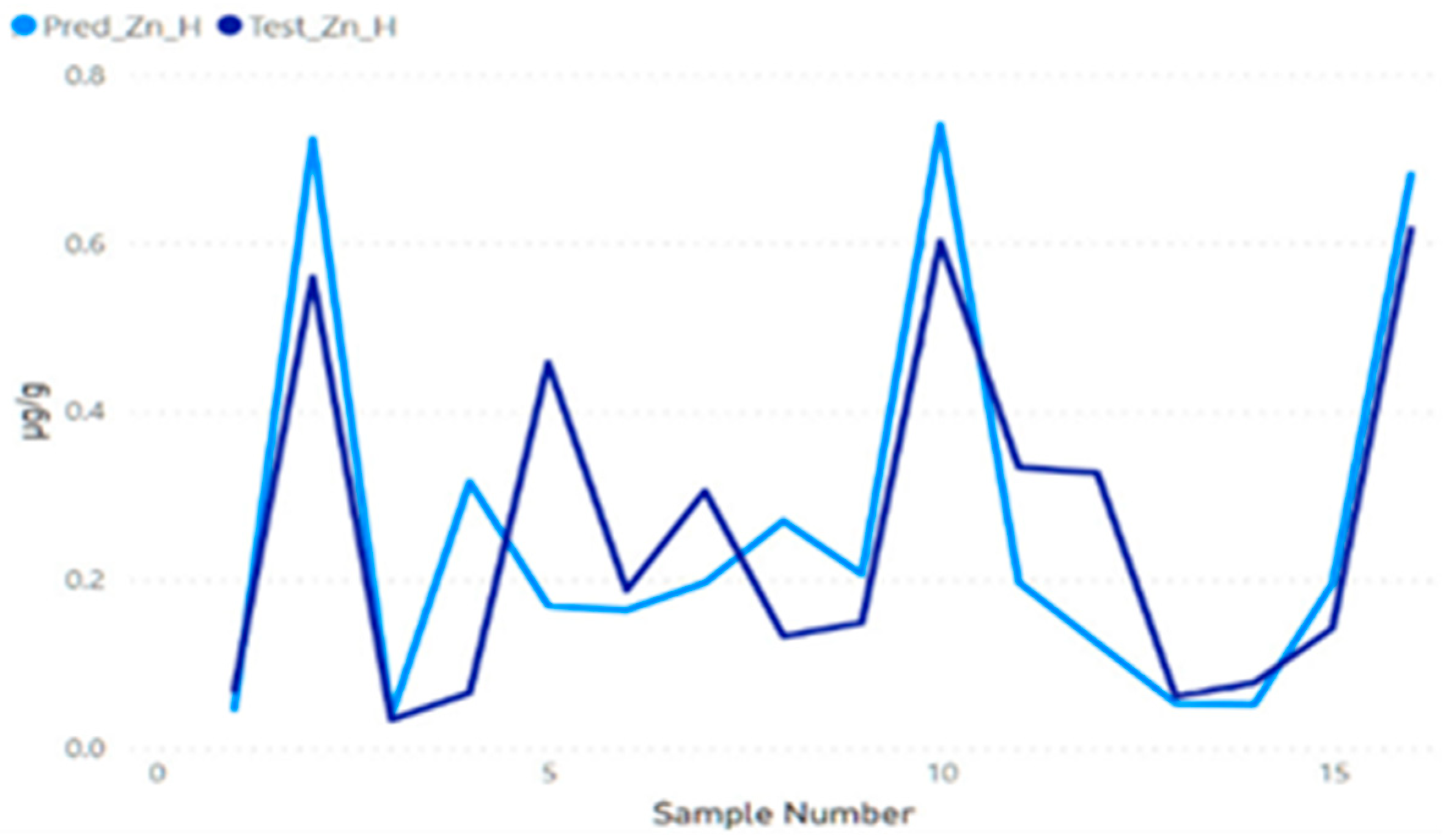
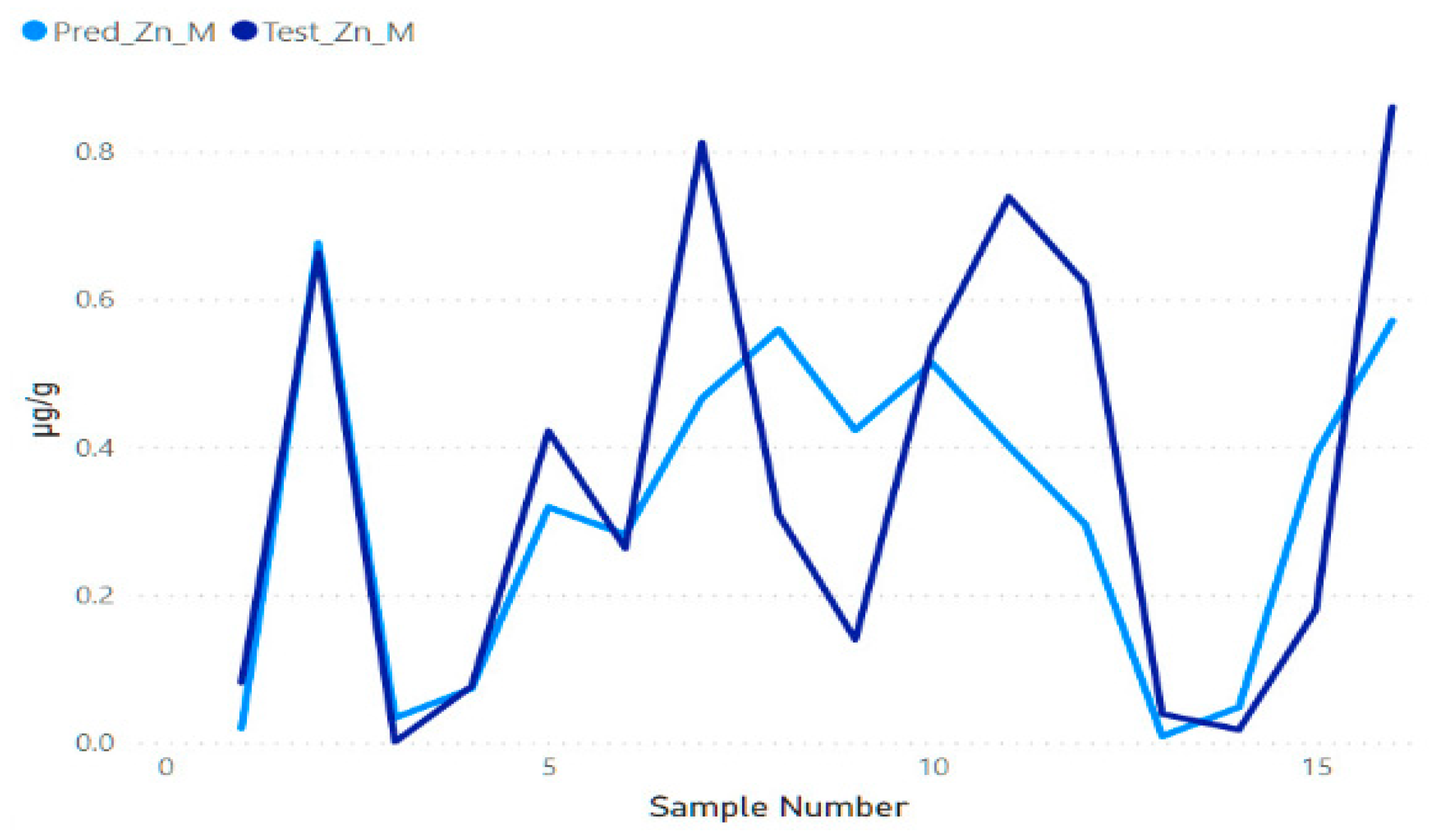
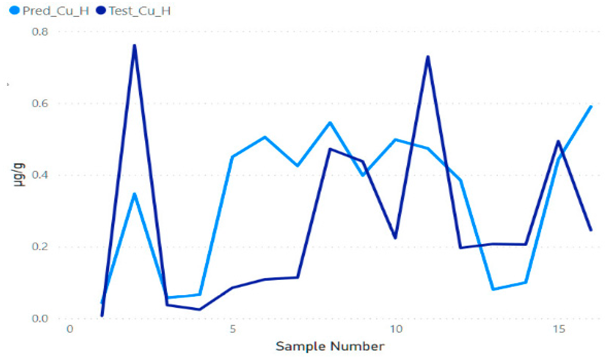
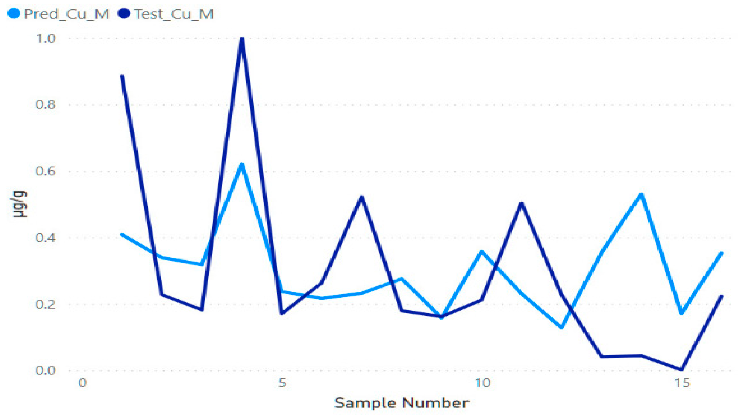
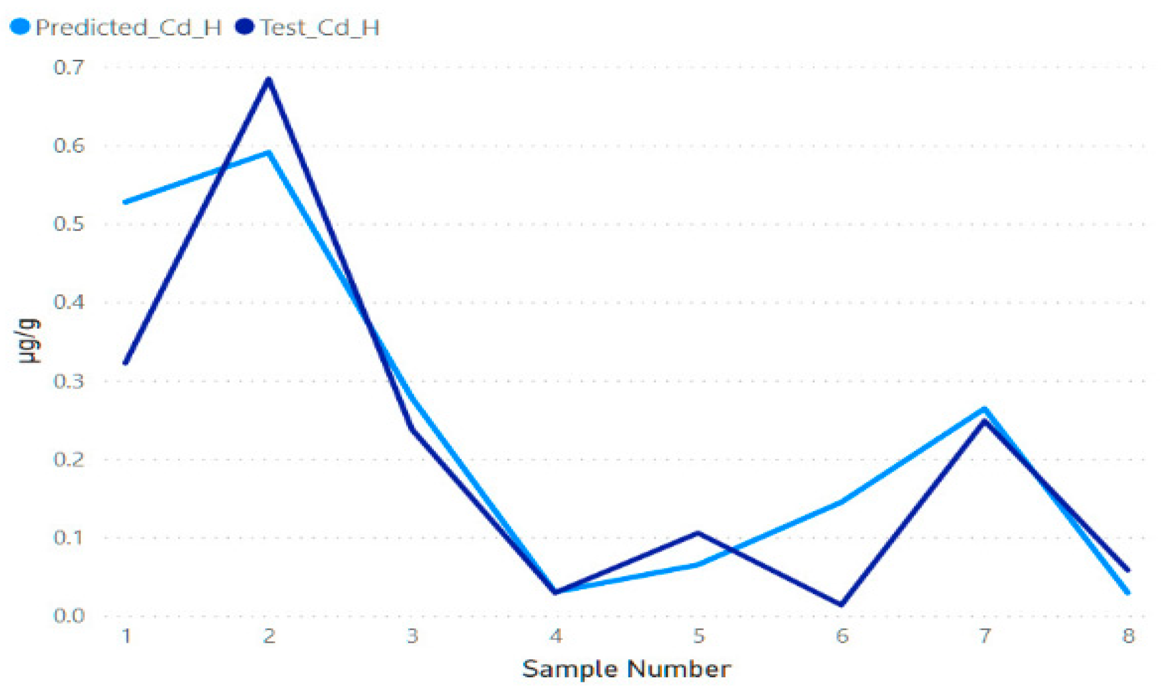
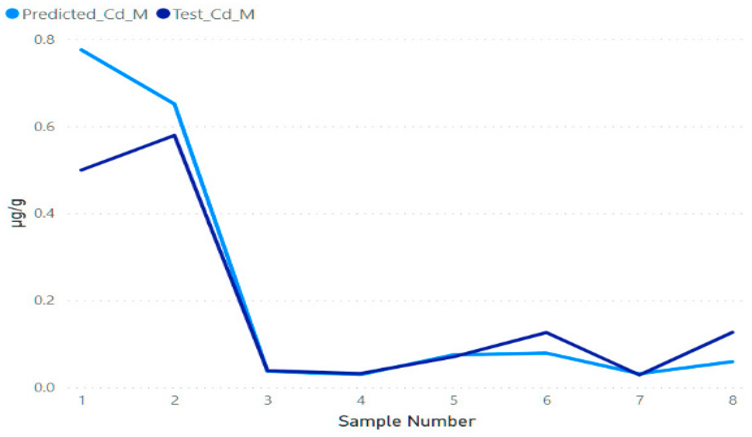
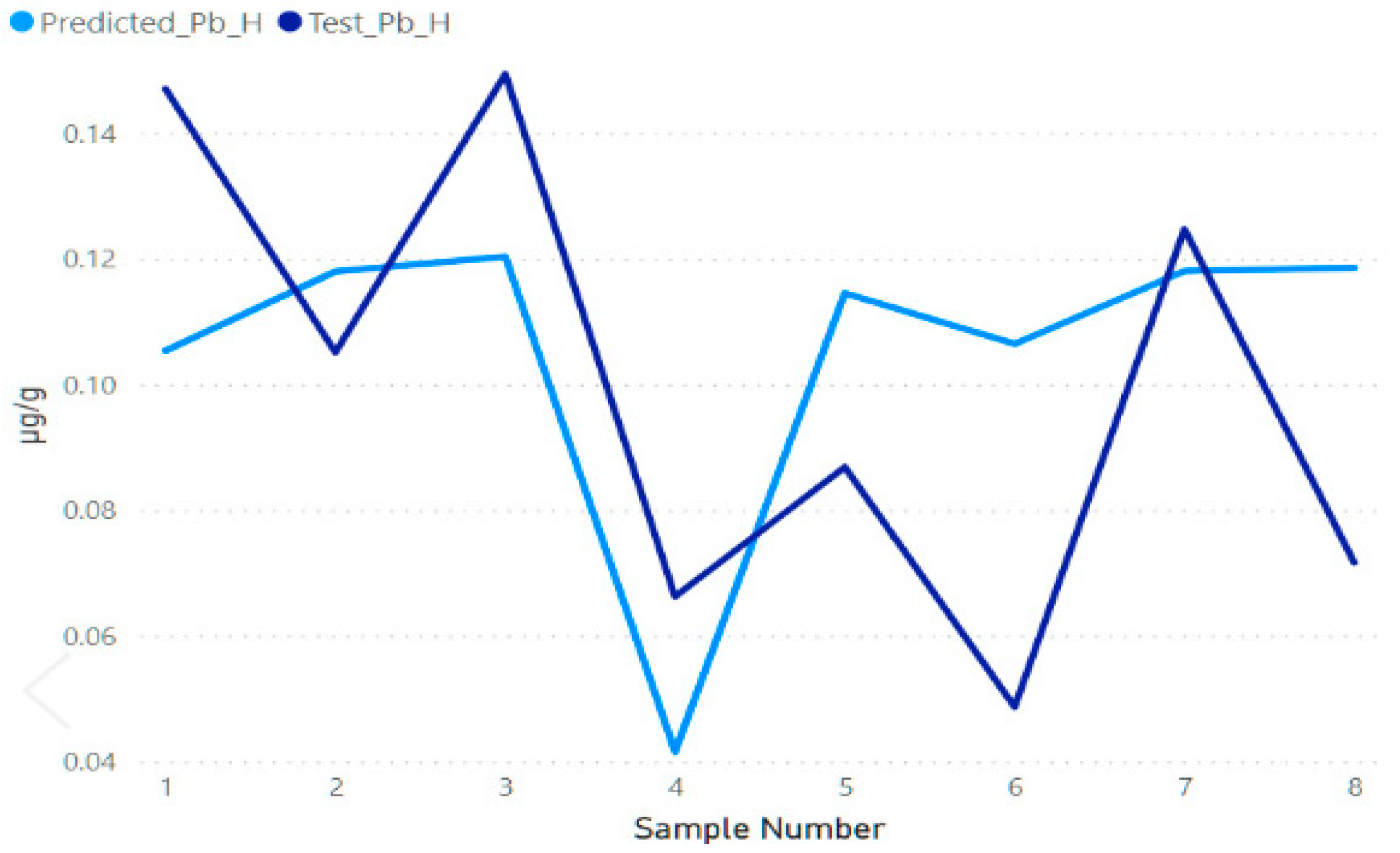
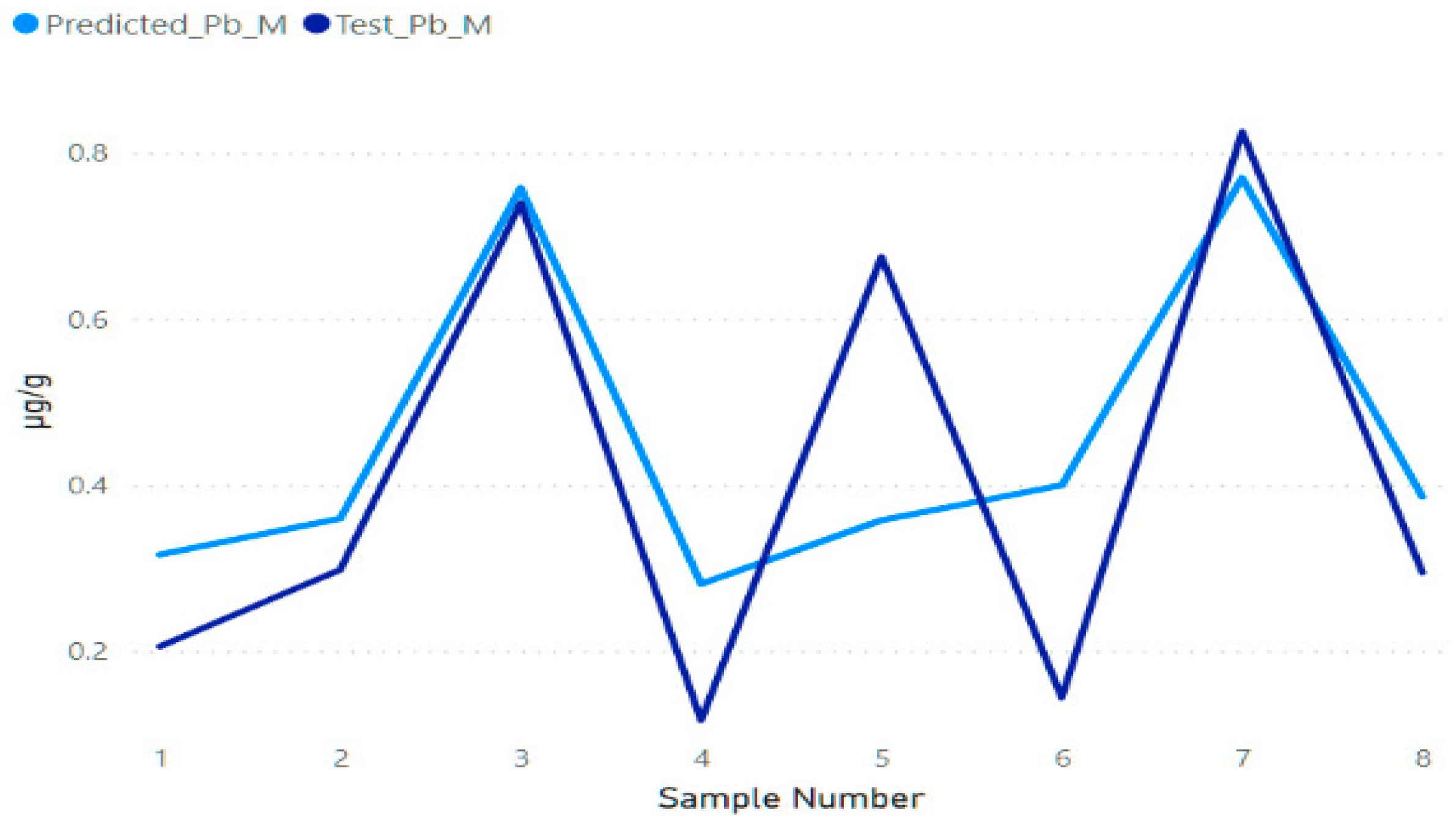
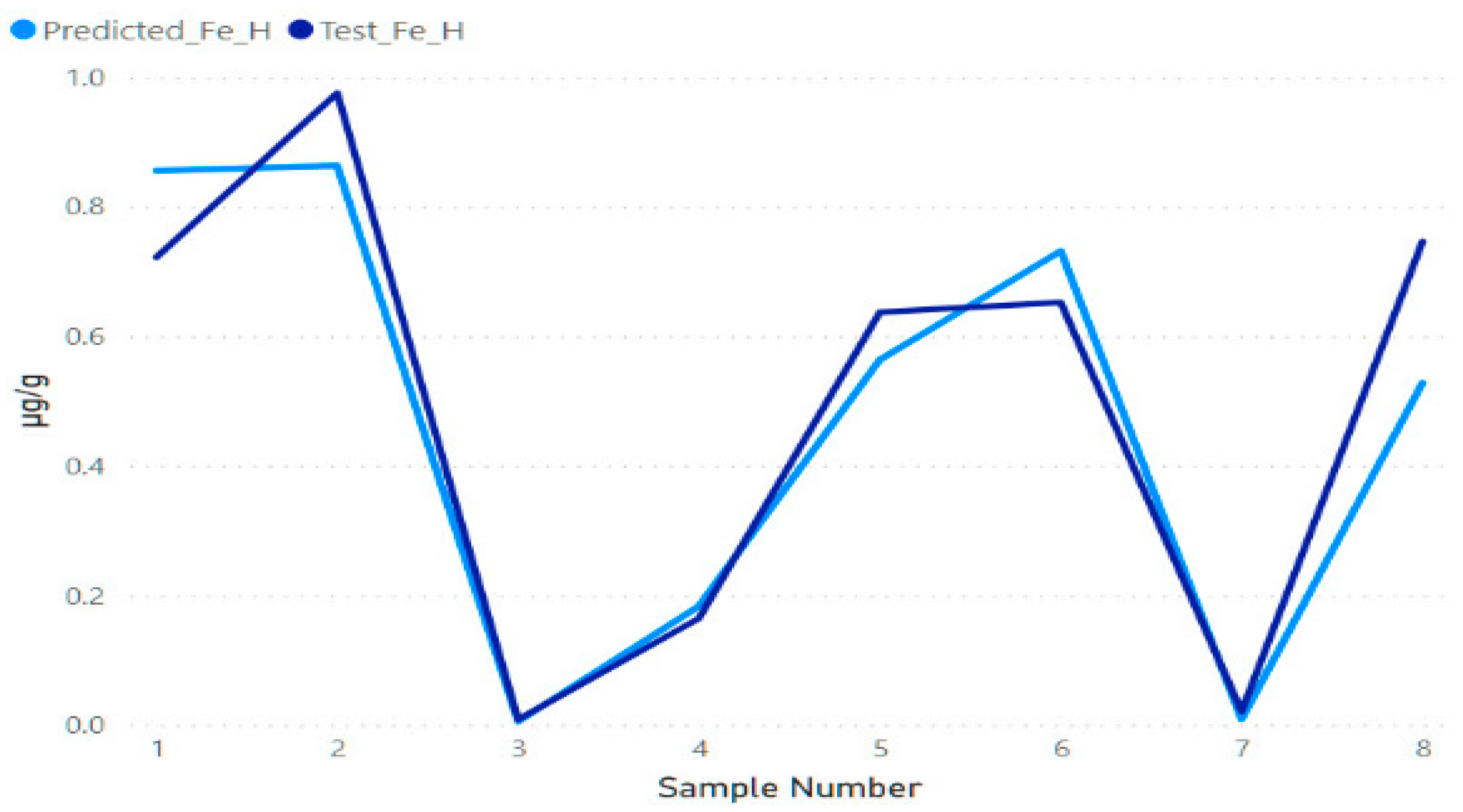
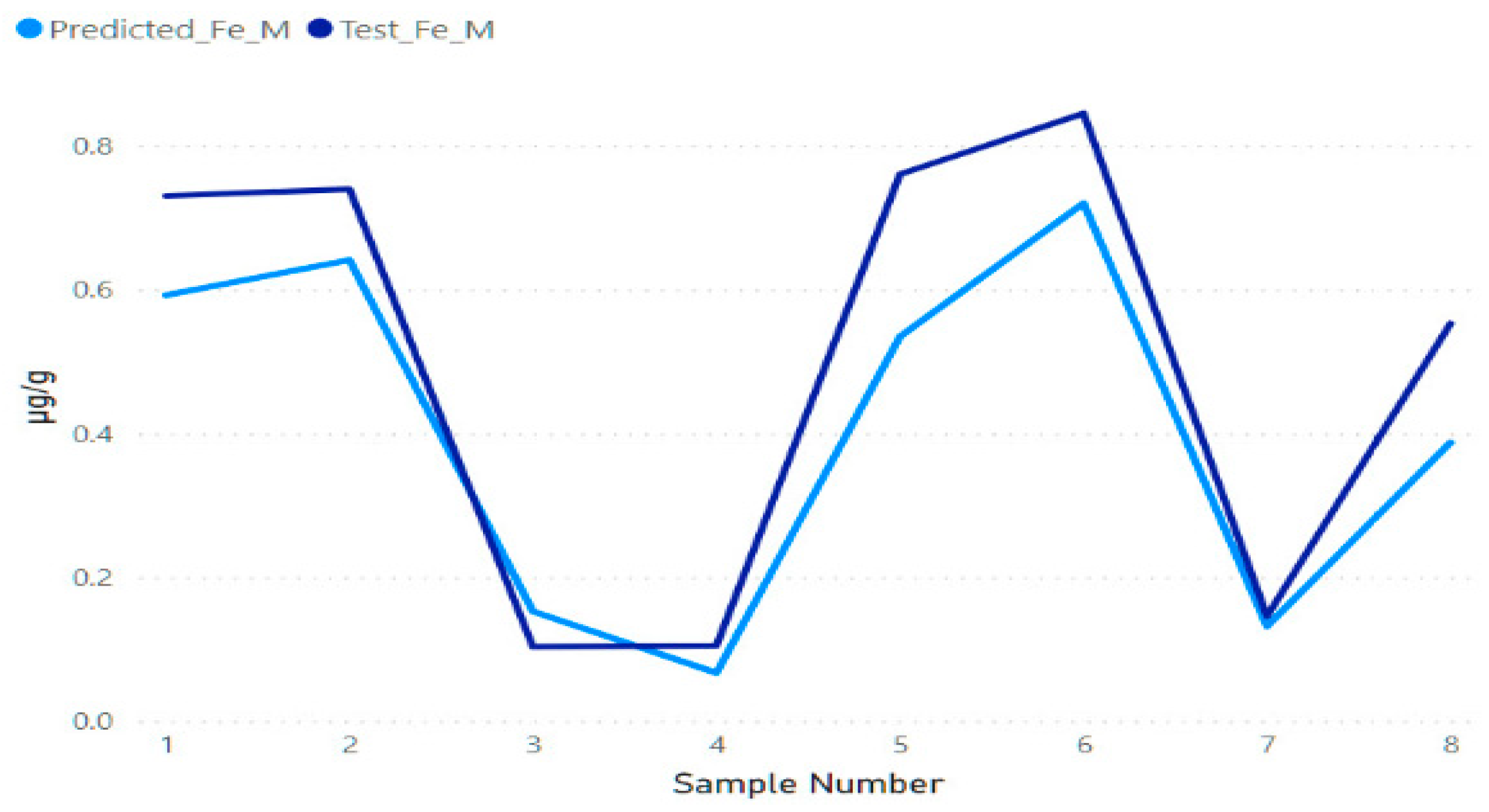
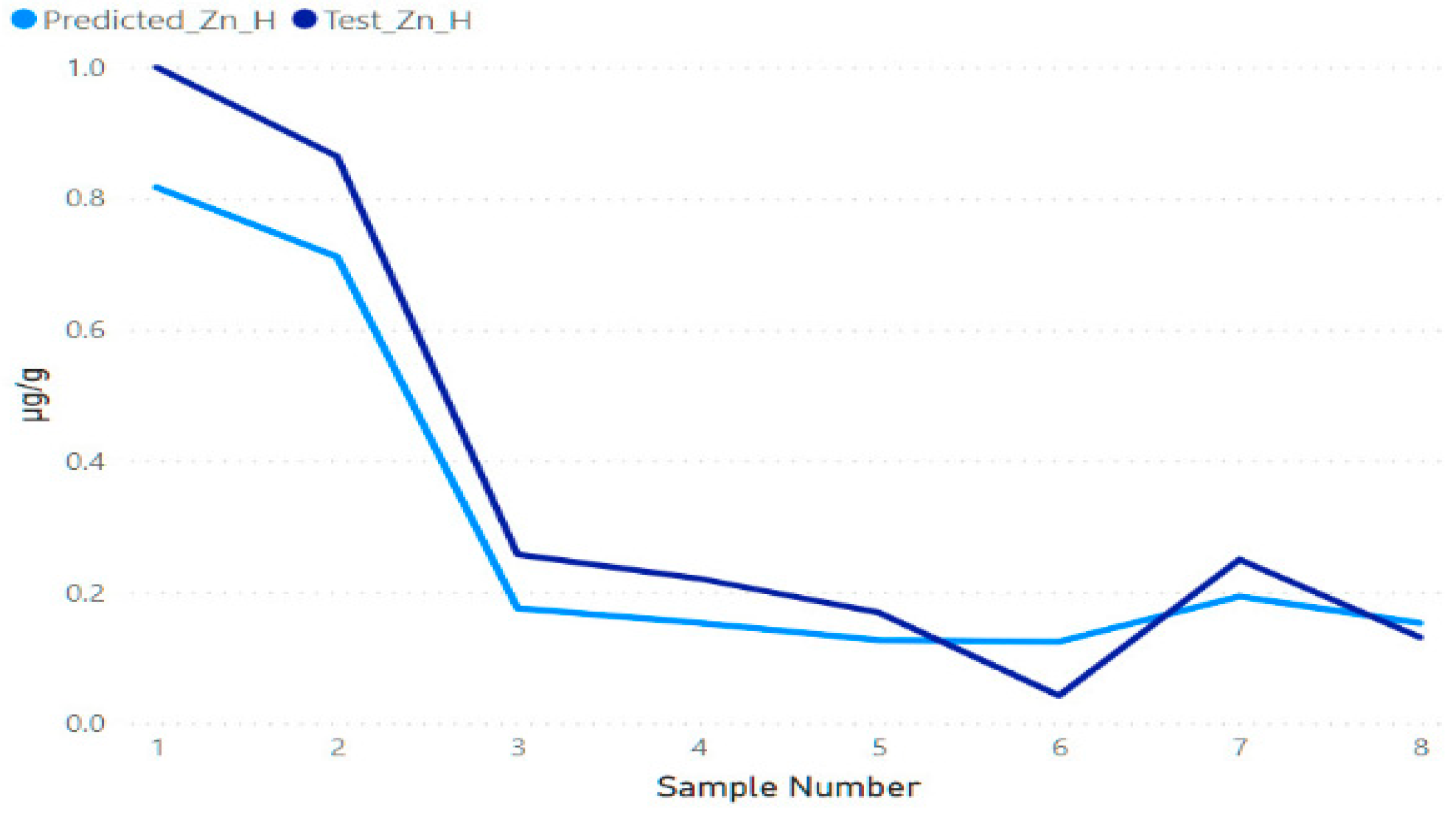
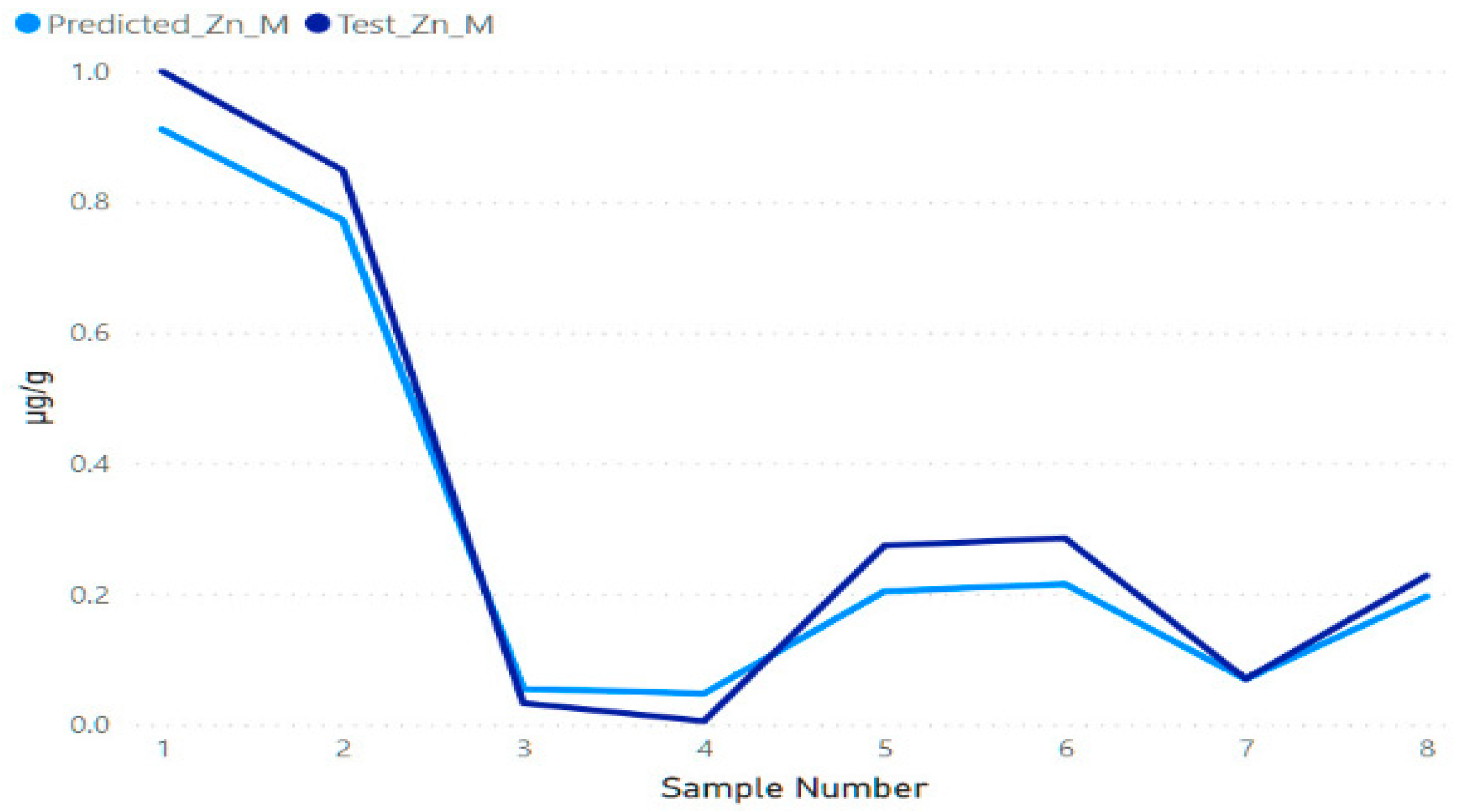
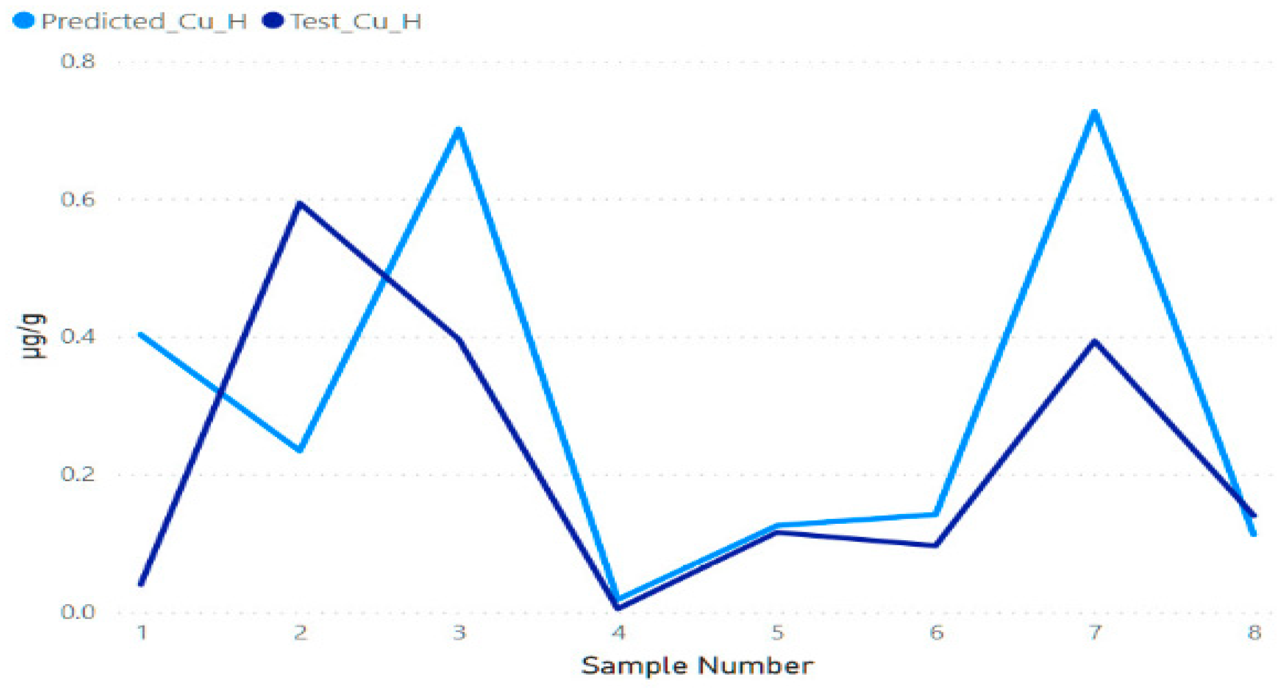
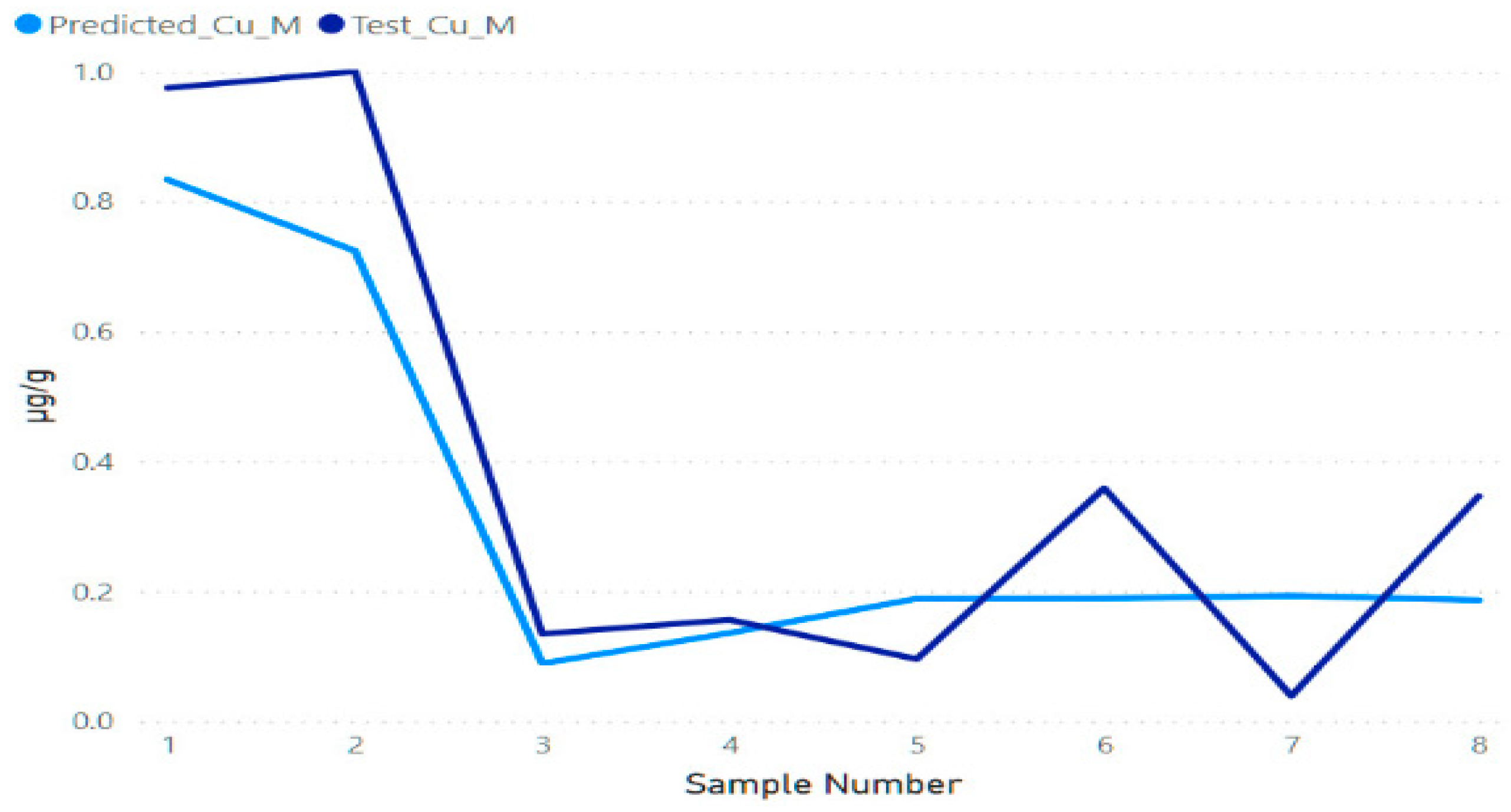
Appendix C. Random Forest—Actual Values vs. Predicted Values for the Test Dataset

Figure A5. Prediction of Cd concentration for fish hepatic tissues—actual values vs. predicted value, at BS coast.
Sustainability 13 08936 g0a5
Figure A6. Prediction of Cd concentration for fish muscle tissues—actual values vs. predicted value, at BS coast.
Sustainability 13 08936 g0a6
Figure A7. Prediction of Pb concentration for fish hepatic tissues—actual values vs. predicted value, at BS coast.
Sustainability 13 08936 g0a7
Figure A8. Prediction of Pb concentration for fish muscle tissues—actual values vs. predicted value, at BS coast.
Sustainability 13 08936 g0a8
Figure A9. Prediction of Fe concentration for fish hepatic tissues—actual values vs. predicted value, at BS coast.
Sustainability 13 08936 g0a9
Figure A10. Prediction of Fe concentration for fish muscle tissues—actual values vs. predicted value, at BS coast.
Sustainability 13 08936 g0a10
Figure A11. Prediction of Zn concentration for fish hepatic tissues—actual values vs. predicted value, at BS coast.
Sustainability 13 08936 g0a11
Figure A12. Prediction of Zn concentration for fish muscle tissues—actual values vs. predicted value, at BS coast.
Sustainability 13 08936 g0a12
Figure A13. Prediction of Cu concentration for fish hepatic tissues—actual values vs. predicted value, at BS coast.
Sustainability 13 08936 g0a13
Figure A14. Prediction of Cu concentration for fish muscle tissues—actual values vs. predicted value, at BS coast.
Sustainability 13 08936 g0a14
Figure A15. Prediction of Cd concentration for fish hepatic tissues—actual values vs. predicted value, at DD.
Sustainability 13 08936 g0a15
Figure A16. Prediction of Cd concentration for fish muscle tissues—actual values vs. predicted value, at DD.
Sustainability 13 08936 g0a16
Figure A17. Prediction of Pb concentration for fish hepatic tissues—actual values vs. predicted value, at DD.
Sustainability 13 08936 g0a17
Figure A18. Prediction of Pb concentration for fish muscle tissues—actual values vs. predicted value, at DD.
Sustainability 13 08936 g0a18
Figure A19. Prediction of Fe concentration for fish hepatic tissues—actual values vs. predicted value, at DD.
Sustainability 13 08936 g0a19
Figure A20. Prediction of Fe concentration for fish muscle tissues—actual values vs. predicted value, at DD.
Sustainability 13 08936 g0a20
Figure A21. Prediction of Zn concentration for fish hepatic tissues—actual values vs. predicted value, at DD.
Sustainability 13 08936 g0a21
Figure A22. Prediction of Zn concentration for fish muscle tissues—actual values vs. predicted value, at DD.
Sustainability 13 08936 g0a22
Figure A23. Prediction of Cu concentration for fish hepatic tissues—actual values vs. predicted value, at DD.
Sustainability 13 08936 g0a23
Figure A24. Prediction of Cu concentration for fish muscle tissues—actual values vs. predicted value, at DD.
Sustainability 13 08936 g0a24
Figure A25. Prediction of Cd concentration for fish hepatic tissues—actual values vs. predicted value, at DR.
Sustainability 13 08936 g0a25
Figure A26. Prediction of Cd concentration for fish muscle tissues—actual values vs. predicted value, at DR.
Sustainability 13 08936 g0a26
Figure A27. Prediction of Pb concentration for fish hepatic tissues—actual values vs. predicted value, at DR.
Sustainability 13 08936 g0a27
Figure A28. Prediction of Pb concentration for fish muscle tissues—actual values vs. predicted value, at DR.
Sustainability 13 08936 g0a28
Figure A29. Prediction of Fe concentration for fish hepatic tissues—actual values vs. predicted value, at DR.
Sustainability 13 08936 g0a29
Figure A30. Prediction of Fe concentration for fish muscle tissues—actual values vs. predicted value, at DR.
Sustainability 13 08936 g0a30
Figure A31. Prediction of Zn concentration for fish hepatic tissues—actual values vs. predicted value, at DR.
Sustainability 13 08936 g0a31
Figure A32. Prediction of Zn concentration for fish muscle tissues—actual values vs. predicted value, at DR.
Sustainability 13 08936 g0a32
Figure A33. Prediction of Cu concentration for fish hepatic tissues—actual values vs. predicted value, at DR.
Sustainability 13 08936 g0a33
Figure A34. Prediction of Cu concentration for fish muscle tissues—actual values vs. predicted value, at DR.
Sustainability 13 08936 g0a34

References

  1. Usero, J.; Morillo, J.; Gracia, I. Heavy Metal Concentrations in Molluscs from the Atlantic Coast of Southern Spain. Chemosphere 2005, 59, 1175–1181. [Google Scholar] [CrossRef]
  2. Simionov, I.A.; Cristea, V.; Petrea, S.M.; Mogodan, A.; Nicoara, M.; Baltag, E.S.; Strungaru, S.A.; Faggio, C. Bioconcentration of Essential and Nonessential Elements in Black Sea Turbot (Psetta Maxima Maeotica Linnaeus, 1758) in Relation to Fish Gender. J. Mar. Sci. Eng. 2019, 7, 466. [Google Scholar] [CrossRef] [Green Version]
  3. Petrea, Ș.-M.; Costache, M.; Cristea, D.; Strungaru, Ș.-A.; Simionov, I.-A.; Mogodan, A.; Oprica, L.; Cristea, V. A Machine Learning Approach in Analyzing Bioaccumulation of Heavy Metals in Turbot Tissues. Molecules 2020, 25, 4696. [Google Scholar] [CrossRef] [PubMed]
  4. Simionov, I.A.; Cristea, D.S.; Petrea, S.M.; Mogodan, A.; Nicoara, M.; Plavan, G.; Baltag, E.S.; Jijie, R.; Strungaru, S.A. Preliminary Investigation of Lower Danube Pollution Caused by Potentially Toxic Metals. Chemosphere 2021, 264, 128496. [Google Scholar] [CrossRef]
  5. Hu, Z.; Zhang, Y.; Zhao, Y.; Xie, M.; Zhong, J.; Tu, Z.; Liu, J. A Water Quality Prediction Method Based on the Deep LSTM Network Considering Correlation in Smart Mariculture. Sensors 2019, 19, 1420. [Google Scholar] [CrossRef] [Green Version]
  6. Stadnicka, J.; Schirmer, K.; Ashauer, R. Predicting Concentrations of Organic Chemicals in Fish by Using Toxicokinetic Models. Environ. Sci. Technol. 2012, 46, 3273–3280. [Google Scholar] [CrossRef]
  7. Hinojosa-Garro, D.; von Osten, J.R.; Dzul-Caamal, R. Banded Tetra (Astyanax Aeneus) as Bioindicator of Trace Metals in Aquatic Ecosystems of the Yucatan Peninsula, Mexico: Experimental Biomarkers Validation and Wild Populations Biomonitoring. Ecotoxicol. Environ. Saf. 2020, 195, 110477. [Google Scholar] [CrossRef] [PubMed]
  8. Robea, M.A.; Jijie, R.; Nicoara, M.; Plavan, G.; Ciobica, A.S.; Solcan, C.; Audira, G.; Hsiao, C.-D.; Strungaru, S.-A. Vitamin c Attenuates Oxidative Stress and Behavioral Abnormalities Triggered by Fipronil and Pyriproxyfen Insecticide Chronic Exposure on Zebrafish Juvenile. Antioxidants 2020, 9, 944. [Google Scholar] [CrossRef]
  9. Strungaru, S.A.; Plavan, G.; Ciobica, A.; Nicoara, M.; Robea, M.A.; Solcan, C.; Todirascu-Ciornea, E.; Petrovici, A. Acute Exposure to Gold Induces Fast Changes in Social Behavior and Oxidative Stress of Zebrafish (Danio rerio). J. Trace Elem. Med. Biol. 2018, 50, 249–256. [Google Scholar] [CrossRef] [PubMed]
  10. Akinsanya, B.; Ayanda, I.O.; Fadipe, A.O.; Onwuka, B.; Saliu, J.K. Heavy Metals, Parasitologic and Oxidative Stress Biomarker Investigations in Heterotis Niloticus from Lekki Lagoon, Lagos, Nigeria. Toxicol. Rep. 2020, 7, 1075–1082. [Google Scholar] [CrossRef] [PubMed]
  11. Robea, M.A.; Balmus, I.M.; Ciobica, A.; Strungaru, S.; Plavan, G.; Gorgan, L.D.; Savuca, A.; Nicoara, M. Parkinson’s Disease-Induced Zebrafish Models: Focussing on Oxidative Stress Implications and Sleep Processes. Oxid. Med. Cell. Longev. 2020, 2020, 1370837. [Google Scholar] [CrossRef]
  12. Oliva, M.; José Vicente, J.; Gravato, C.; Guilhermino, L.; Dolores Galindo-Riaño, M. Oxidative Stress Biomarkers in Senegal Sole, Solea senegalensis, to Assess the Impact of Heavy Metal Pollution in a Huelva Estuary (SW Spain): Seasonal and Spatial Variation. Ecotoxicol. Environ. Saf. 2012, 75, 151–162. [Google Scholar] [CrossRef] [PubMed]
  13. Strungaru, S.A.; Robea, M.A.; Plavan, G.; Todirascu-Ciornea, E.; Ciobica, A.; Nicoara, M. Acute Exposure to Methylmercury Chloride Induces Fast Changes in Swimming Performance, Cognitive Processes and Oxidative Stress of Zebrafish (Danio Rerio) as Reference Model for Fish Community. J. Trace Elem. Med. Biol. 2018, 47, 115–123. [Google Scholar] [CrossRef]
  14. Adeogun, A.O.; Ibor, O.R.; Omiwole, R.; Chukwuka, A.V.; Adewale, A.H.; Kumuyi, O.; Arukwe, A. Sex-Differences in Physiological and Oxidative Stress Responses and Heavy Metals Burden in the Black Jaw Tilapia, Sarotherodon melanotheron from a Tropical Freshwater Dam (Nigeria). Comp. Biochem. Physiol. Part C Toxicol. Pharmacol. 2020, 229, 108676. [Google Scholar] [CrossRef] [PubMed]
  15. Santovito, G.; Trentin, E.; Gobbi, I.; Bisaccia, P.; Tallandini, L.; Irato, P. Non-Enzymatic Antioxidant Responses of Mytilus galloprovincialis: Insights into the Physiological Role against Metal-Induced Oxidative Stress. Comp. Biochem. Physiol. Part C Toxicol. Pharmacol. 2021, 240, 108909. [Google Scholar] [CrossRef] [PubMed]
  16. AbdElgawad, H.; Zinta, G.; Hamed, B.A.; Selim, S.; Beemster, G.; Hozzein, W.N.; Wadaan, M.A.M.; Asard, H.; Abuelsoud, W. Maize Roots and Shoots Show Distinct Profiles of Oxidative Stress and Antioxidant Defense under Heavy Metal Toxicity. Environ. Pollut. 2020, 258, 113705. [Google Scholar] [CrossRef]
  17. Paithankar, J.G.; Saini, S.; Dwivedi, S.; Sharma, A.; Chowdhuri, D.K. Heavy Metal Associated Health Hazards: An Interplay of Oxidative Stress and Signal Transduction. Chemosphere 2021, 262, 128350. [Google Scholar] [CrossRef]
  18. Yan, X.; Wang, J.; Zhu, L.; Wang, J.; Li, S.; Kim, Y.M. Oxidative Stress, Growth Inhibition, and DNA Damage in Earthworms Induced by the Combined Pollution of Typical Neonicotinoid Insecticides and Heavy Metals. Sci. Total Environ. 2021, 754, 141873. [Google Scholar] [CrossRef]
  19. Xu, J.; Zhao, M.; Pei, L.; Liu, X.; Wei, L.; Li, A.; Mei, Y.; Xu, Q. Effects of Heavy Metal Mixture Exposure on Hematological and Biomedical Parameters Mediated by Oxidative Stress. Sci. Total Environ. 2020, 705, 134865. [Google Scholar] [CrossRef]
  20. Saleh, Y.S.; Marie, M.A.S. Use of Arius Thalassinus Fish in a Pollution Biomonitoring Study, Applying Combined Oxidative Stress, Hematology, Biochemical and Histopathological Biomarkers: A Baseline Field Study. Mar. Pollut. Bull. 2016, 106, 308–322. [Google Scholar] [CrossRef]
  21. Mohanty, D.; Samanta, L. Multivariate Analysis of Potential Biomarkers of Oxidative Stress in Notopterus Notopterus Tissues from Mahanadi River as a Function of Concentration of Heavy Metals. Chemosphere 2016, 155, 28–38. [Google Scholar] [CrossRef]
  22. Yogeshwaran, A.; Gayathiri, K.; Muralisankar, T.; Gayathri, V.; Monica, J.I.; Rajaram, R.; Marimuthu, K.; Bhavan, P.S. Bioaccumulation of Heavy Metals, Antioxidants, and Metabolic Enzymes in the Crab Scylla serrata from Different Regions of Tuticorin, Southeast Coast of India. Mar. Pollut. Bull. 2020, 158, 111443. [Google Scholar] [CrossRef] [PubMed]
  23. Mejdoub, Z.; Fahde, A.; Loutfi, M.; Kabine, M. Oxidative Stress Responses of the Mussel Mytilus galloprovincialis Exposed to Emissary’s Pollution in Coastal Areas of Casablanca. Ocean Coast. Manag. 2017, 136, 95–103. [Google Scholar] [CrossRef]
  24. Prokić, M.D.; Borković-Mitić, S.S.; Krizmanić, I.I.; Mutić, J.J.; Vukojević, V.; Nasia, M.; Gavrić, J.P.; Despotović, S.G.; Gavrilović, B.R.; Radovanović, T.B.; et al. Antioxidative Responses of the Tissues of Two Wild Populations of Pelophylax Kl. Esculentus Frogs to Heavy Metal Pollution. Ecotoxicol. Environ. Saf. 2016, 128, 21–29. [Google Scholar] [CrossRef]
  25. Aljbour, S.M.; Al-Horani, F.A.; Kunzmann, A. Metabolic and Oxidative Stress Responses of the Jellyfish Cassiopea to Pollution in the Gulf of Aqaba, Jordan. Mar. Pollut. Bull. 2018, 130, 271–278. [Google Scholar] [CrossRef]
  26. Abarikwu, S.O.; Essien, E.B.; Iyede, O.O.; John, K.; Mgbudom-Okah, C. Biomarkers of Oxidative Stress and Health Risk Assessment of Heavy Metal Contaminated Aquatic and Terrestrial Organisms by Oil Extraction Industry in Ogale, Nigeria. Chemosphere 2017, 185, 412–422. [Google Scholar] [CrossRef] [PubMed]
  27. Tabrez, S.; Zughaibi, T.A.; Javed, M. Bioaccumulation of Heavy Metals and Their Toxicity Assessment in Mystus Species. Saudi J. Biol. Sci. 2021, 28, 1459–1464. [Google Scholar] [CrossRef]
  28. Burgos-Aceves, M.A.; Cohen, A.; Smith, Y.; Faggio, C. MicroRNAs and Their Role on Fish Oxidative Stress during Xenobiotic Environmental Exposures. Ecotoxicol. Environ. Saf. 2018, 148, 995–1000. [Google Scholar] [CrossRef]
  29. Hermenean, A.; Damache, G.; Albu, P.; Ardelean, A.; Ardelean, G.; Puiu Ardelean, D.; Horge, M.; Nagy, T.; Braun, M.; Zsuga, M.; et al. Histopatological Alterations and Oxidative Stress in Liver and Kidney of Leuciscus cephalus Following Exposure to Heavy Metals in the Tur River, North Western Romania. Ecotoxicol. Environ. Saf. 2015, 119, 198–205. [Google Scholar] [CrossRef]
  30. Fatima, M.; Usmani, N.; Firdaus, F.; Zafeer, M.F.; Ahmad, S.; Akhtar, K.; Dawar Husain, S.M.; Ahmad, M.H.; Anis, E.; Mobarak Hossain, M. In Vivo Induction of Antioxidant Response and Oxidative Stress Associated with Genotoxicity and Histopathological Alteration in Two Commercial Fish Species Due to Heavy Metals Exposure in Northern India (Kali) River. Comp. Biochem. Physiol. Part C Toxicol. Pharmacol. 2015, 176–177, 17–30. [Google Scholar] [CrossRef] [PubMed]
  31. Beg, M.U.; Al-Jandal, N.; Al-Subiai, S.; Karam, Q.; Husain, S.; Butt, S.A.; Ali, A.; Al-Hasan, E.; Al-Dufaileej, S.; Al-Husaini, M. Metallothionein, Oxidative Stress and Trace Metals in Gills and Liver of Demersal and Pelagic Fish Species from Kuwaits’ Marine Area. Mar. Pollut. Bull. 2015, 100, 662–672. [Google Scholar] [CrossRef]
  32. Javed, M.; Abbas, K.; Ahmed, T.; Abdullah, S.; Naz, H.; Amjad, H. Metal Pollutants Induced Peroxidase Activity in Different Body Tissues of Freshwater Fish, Labeo Rohita. Environ. Chem. Ecotoxicol. 2020, 2, 162–167. [Google Scholar] [CrossRef]
  33. Pillet, M.; Castaldo, G.; De Weggheleire, S.; Bervoets, L.; Blust, R.; De Boeck, G. Limited Oxidative Stress in Common Carp (Cyprinus Carpio, L., 1758) Exposed to a Sublethal Tertiary (Cu, Cd and Zn) Metal Mixture. Comp. Biochem. Physiol. Part C Toxicol. Pharmacol. 2019, 218, 70–80. [Google Scholar] [CrossRef] [PubMed]
  34. Weber, A.A.; Sales, C.F.; de Souza Faria, F.; Melo, R.M.C.; Bazzoli, N.; Rizzo, E. Effects of Metal Contamination on Liver in Two Fish Species from a Highly Impacted Neotropical River: A Case Study of the Fundão Dam, Brazil. Ecotoxicol. Environ. Saf. 2020, 190, 110165. [Google Scholar] [CrossRef] [PubMed]
  35. Chang, X.; Chen, Y.; Feng, J.; Huang, M.; Zhang, J. Amelioration of Cd-Induced Bioaccumulation, Oxidative Stress and Immune Damage by Probiotic Bacillus coagulans in Common Carp (Cyprinus carpio L.). Aquac. Rep. 2021, 20, 100678. [Google Scholar] [CrossRef]
  36. Xu, Y.H.; Hogstrand, C.; Xu, Y.C.; Zhao, T.; Zheng, H.; Luo, Z. Environmentally Relevant Concentrations of Oxytetracycline and Copper Increased Liver Lipid Deposition through Inducing Oxidative Stress and Mitochondria Dysfunction in Grass Carp Ctenopharyngodon idella. Environ. Pollut. 2021, 283, 117079. [Google Scholar] [CrossRef] [PubMed]
  37. Abdel Rahman, A.N.; ElHady, M.; Hassanin, M.E.; Mohamed, A.A.R. Alleviative Effects of Dietary Indian Lotus Leaves on Heavy Metals-Induced Hepato-Renal Toxicity, Oxidative Stress, and Histopathological Alterations in Nile Tilapia, Oreochromis niloticus (L.). Aquaculture 2019, 509, 198–208. [Google Scholar] [CrossRef]
  38. Hajirezaee, S.; Ajdari, A.; Azhang, B. Metabolite Profiling, Histological and Oxidative Stress Responses in the Grey Mullet, Mugil cephalus Exposed to the Environmentally Relevant Concentrations of the Heavy Metal, Pb (NO3)2. Comp. Biochem. Physiol. Part C Toxicol. Pharmacol. 2021, 244, 109004. [Google Scholar] [CrossRef] [PubMed]
  39. Kakade, A.; Salama, E.S.; Pengya, F.; Liu, P.; Li, X. Long-Term Exposure of High Concentration Heavy Metals Induced Toxicity, Fatality, and Gut Microbial Dysbiosis in Common Carp, Cyprinus carpio. Environ. Pollut. 2020, 266, 115293. [Google Scholar] [CrossRef]
  40. Ning, Y.; Zhou, H.; Wang, E.; Jin, C.; Yu, Y.; Cao, X.; Zhou, D. Study of Cadmium (Cd)-Induced Oxidative Stress in Eisenia fetida Based on Mathematical Modelling. Pedosphere 2021, 31, 460–470. [Google Scholar] [CrossRef]
  41. Gao, Y.; Kang, L.; Zhang, Y.; Feng, J.; Zhu, L. Toxicokinetic and Toxicodynamic (TK-TD) Modeling to Study Oxidative Stress-Dependent Toxicity of Heavy Metals in Zebrafish. Chemosphere 2019, 220, 774–782. [Google Scholar] [CrossRef] [PubMed]
  42. Sahlo, A.T.; Ewees, A.A.; Hemdan, A.M.; Hassanien, A.E. Training of Feedforward Neural Networks Using Sine-Cosine Algorithm to Improve the Prediction of Liver Enzymes on FIsh Farmed on Nano-Selenite. In Proceedings of the 2016 12th International Computer Engineering Conference (ICENCO 2016): Boundless Smart Societies, Cairo, Egypt, 28–29 December 2016. [Google Scholar]
  43. Bethel, B.J.; Buravleva, Y.; Tang, D. Blue Economy and Blue Activities: Opportunities, Challenges, and Recommendations for The Bahamas. Water 2021, 13, 1399. [Google Scholar] [CrossRef]
  44. Tianming, G.; Bobylev, N.; Gadal, S.; Lagutina, M.; Sergunin, A.; Erokhin, V. Planning for Sustainability: An Emerging Blue Economy in Russia’s Coastal Arctic? Sustainability 2021, 13, 4957. [Google Scholar] [CrossRef]
  45. Lin, D.; Liu, K.; Chen, X. Rapid Detection of Heavy Metal-Contaminated Tegillarca Granosa Using near Infrared Spectroscopy. J. Chin. Inst. Food Sci. Technol. 2015, 15. [Google Scholar] [CrossRef]
  46. Rodríguez-Bermúdez, R.; Herrero-Latorre, C.; López-Alonso, M.; Losada, D.E.; Iglesias, R.; Miranda, M. Organic Cattle Products: Authenticating Production Origin by Analysis of Serum Mineral Content. Food Chem. 2018, 264, 210–217. [Google Scholar] [CrossRef] [PubMed]
  47. Zhang, H.; Yin, A.; Yang, X.; Fan, M.; Shao, S.; Wu, J.; Wu, P.; Zhang, M.; Gao, C. Use of Machine-Learning and Receptor Models for Prediction and Source Apportionment of Heavy Metals in Coastal Reclaimed Soils. Ecol. Indic. 2021, 122, 107233. [Google Scholar] [CrossRef]
  48. Tan, K.; Ma, W.; Wu, F.; Du, Q. Random Forest–Based Estimation of Heavy Metal Concentration in Agricultural Soils with Hyperspectral Sensor Data. Environ. Monit. Assess. 2019, 191, 446. [Google Scholar] [CrossRef]
  49. Park, H.; Kim, K. Comparisons among Machine Learning Models for the Prediction of Hypercholestrolemia Associated with Exposure to Lead, Mercury, and Cadmium. Int. J. Environ. Res. Public Health 2019, 16, 2666. [Google Scholar] [CrossRef] [Green Version]
  50. Victoriano, J.M.; Lacatan, L.L.; Vinluan, A.A. Predicting River Pollution Using Random Forest Decision Tree with GIS Model: A Case Study of MMORS, Philippines. Int. J. Environ. Sci. Dev. 2020, 11, 36–42. [Google Scholar] [CrossRef] [Green Version]
  51. Calmuc, M.; Calmuc, V.; Arseni, M.; Topa, C.; Timofti, M.; Georgescu, L.P.; Iticescu, C. A Comparative Approach to a Series of Physico-Chemical Quality Indices Used in Assessing Water Quality in the Lower Danube. Water 2020, 12, 3239. [Google Scholar] [CrossRef]
  52. Wątor, K.; Zdechlik, R. Application of Water Quality Indices to the Assessment of the Effect of Geothermal Water Discharge on River Water Quality—Case Study from the Podhale Region (Southern Poland). Ecol. Indic. 2021, 121, 107098. [Google Scholar] [CrossRef]
  53. Al-Hussaini, S.N.H.; Al-Obaidy, A.H.M.J.; Al-Mashhady, A.A.M. Environmental Assessment of Heavy Metal Pollution of Diyala River within Baghdad City. Appl. Water Sci. 2018, 8, 87. [Google Scholar] [CrossRef] [Green Version]
  54. Simionov, I.-A.; Cristea, V.; Petrea, S.-M.; Mogodan, A.; Nica, A.; Strungaru, S.-A.; Ene, A.; Sarpe, D.-A. Heavy metal evaluation in the lower sector of Danube River. Sci. Pap. Ser. E Land Reclam. Earth Obs. Surv. Environ. Eng. 2020, 9, 11–16. [Google Scholar]
  55. Strungaru, S.A.; Nicoara, M.; Jitar, O.; Plavan, G. Influence of Urban Activity in Modifying Water Parameters, Concentration and Uptake of Heavy Metals in Typha Latifolia L. into a River That Crosses an Industrial City. J. Environ. Health Sci. Eng. 2015, 13, 5. [Google Scholar] [CrossRef] [PubMed] [Green Version]
  56. Plavan, G.; Jitar, O.; Teodosiu, C.; Nicoara, M.; Micu, D.; Strungaru, S.A. Toxic Metals in Tissues of Fishes from the Black Sea and Associated Human Health Risk Exposure. Environ. Sci. Pollut. Res. 2017, 24, 7776–7787. [Google Scholar] [CrossRef] [PubMed]
  57. Jijie, R.; Solcan, G.; Nicoara, M.; Micu, D.; Strungaru, S.A. Antagonistic Effects in Zebrafish (Danio Rerio) Behavior and Oxidative Stress Induced by Toxic Metals and Deltamethrin Acute Exposure. Sci. Total Environ. 2020, 698, 134299. [Google Scholar] [CrossRef]
  58. Zhang, Z. Variable Selection with Stepwise and Best Subset Approaches. Ann. Transl. Med. 2016, 4, 136. [Google Scholar] [CrossRef] [Green Version]
  59. Kamble, V.B.; Deshmukh, S.N. Comparision Between Accuracy and MSE, RMSE by Using Proposed Method with Imputation Technique. Orient. J. Comput. Sci. Technol. 2017, 10, 773–779. [Google Scholar] [CrossRef] [Green Version]
  60. Sagi, O.; Rokach, L. Ensemble Learning: A Survey. Wiley Interdiscip. Rev. Data Min. Knowl. Discov. 2018, 8, e1249. [Google Scholar] [CrossRef]
  61. Freidman, J.H. Greedy Function Approximation: A Gradient Boosting Machine. Ann. Stat. 2001, 29, 1189–1232. [Google Scholar]
  62. Breiman, L. Random Forests. Mach. Learn. 2001, 45, 5–32. [Google Scholar] [CrossRef] [Green Version]
  63. Bentéjac, C.; Csörgő, A.; Martínez-Muñoz, G. A Comparative Analysis of Gradient Boosting Algorithms. Artif. Intell. Rev. 2021, 54, 1937–1967. [Google Scholar] [CrossRef]
  64. Luo, M.; Wang, Y.; Xie, Y.; Zhou, L.; Qiao, J.; Qiu, S.; Sun, Y. Combination of Feature Selection and Catboost for Prediction: The First Application to the Estimation of Aboveground Biomass. Forests 2021, 12, 216. [Google Scholar] [CrossRef]
  65. Scornet, E.; Biau, G.; Vert, J.P. Consistency of Random Forests. Ann. Stat. 2015, 43, 1716–1741. [Google Scholar] [CrossRef]
  66. Breiman, L.; Friedman, J.H.; Olshen, R.A.; Stone, C.J. Classification and Regression Trees; Routledge: London, UK, 2017; ISBN 9781351460491. [Google Scholar]
  67. Athey, S.; Tibshirani, J.; Wager, S. Generalized Random Forests. Ann. Stat. 2019, 47, 1148–1178. [Google Scholar] [CrossRef] [Green Version]
  68. Ziegel, E.R. The Elements of Statistical Learning. Technometrics 2003, 45, 267–268. [Google Scholar] [CrossRef]
  69. Grömping, U. Variable Importance in Regression Models. Wiley Interdiscip. Rev. Comput. Stat. 2015, 7, 137–152. [Google Scholar] [CrossRef]
  70. Boulesteix, A.L.; Janitza, S.; Hapfelmeier, A.; Van Steen, K.; Strobl, C. Letter to the Editor: On the Term “interaction” and Related Phrases in the Literature on Random Forests. Brief. Bioinform. 2015, 16, 338–345. [Google Scholar] [CrossRef] [PubMed]
  71. Verikas, A.; Gelzinis, A.; Bacauskiene, M. Mining Data with Random Forests: A Survey and Results of New Tests. Pattern Recognit. 2011, 44, 330–349. [Google Scholar] [CrossRef]
  72. Gasparotti, C. The Main Factors of Water Pollution in Danube River Basin. Euro Econ. 2014, 33, 91–106. [Google Scholar]
  73. Popescu, I. Fisheries in the Black Sea; European Parliament: Brussels, Belgium, 2010.
  74. Sommerhäuser, M.; Robert, S.; Birk, S.; Hering, D.; Moog, O.; Stubauer, I.; Ofenböck, T. UNDP/GEF Danube Regional Project “Strengthening The Implementation Capacities For Nutrient Reduction And Transboundary Cooperation In The Danube River Basin” Activity 1.1.6 “Developing The Typology Of Surface Waters and Defining The Relevant Reference Conditions.”. University of Duisburg-Essen, Germany and BOKU—University of Natural Resources and Applied Life Science: Vienna, Austria, 2003. Available online: https://www.researchgate.net/publication/270802356_Developing_the_typology_of_surface_waters_and_defining_the_relevant_reference_conditions (accessed on 20 June 2021).
  75. Oaie, G.; Secrieru, D.; Szobotka, Ş.; Fulga, C.; Stănică, A. Danube River: Sedimentological, mineralogical and geochemical characteristics of the bottom sediments. GeoEcoMarina 2005, 11, 77–85. [Google Scholar]
  76. Vignati, D.A.L.; Secrieru, D.; Bogatova, Y.I.; Dominik, J.; Céréghino, R.; Berlinsky, N.A.; Oaie, G.; Szobotka, S.; Stanica, A. Trace Element Contamination in the Arms of the Danube Delta (Romania/Ukraine): Current State of Knowledge and Future Needs. J. Environ. Manag. 2013, 125, 169–178. [Google Scholar] [CrossRef] [Green Version]
  77. WHO. Iron in Drinking-Water. Background Document for Development of WHO Guidelines for Drinking-Water Quality; WHO: Geneva, Switzerland, 2003. [Google Scholar]
  78. European Commision. Directive 2006/1881/EC the Comission of the European Communities Setting Maximum Levels for Certain Contaminants in Foodstuffs; European Commision: Brussels, Belgium, 2006. [Google Scholar]
  79. Brucka-Jastrzȩbska, E. The Effect of Aquatic Cadmium and Lead Pollution on Lipid Peroxidation and Superoxide Dismutase Activity in Freshwater Fish. Pol. J. Environ. Stud. 2010, 19, 1139–1150. [Google Scholar]
  80. Schober, P.; Schwarte, L.A. Correlation Coefficients: Appropriate Use and Interpretation. Anesth. Analg. 2018, 126, 1763–1768. [Google Scholar] [CrossRef]
  81. Rajkowska, M.; Protasowicki, M. Distribution of Metals (Fe, Mn, Zn, Cu) in Fish Tissues in Two Lakes of Different Trophy in Northwestern Poland. Environ. Monit. Assess. 2013, 185, 3493–3502. [Google Scholar] [CrossRef] [Green Version]
  82. Forouhar Vajargah, M.; Mohamadi Yalsuyi, A.; Sattari, M.; Prokić, M.D.; Faggio, C. Effects of Copper Oxide Nanoparticles (CuO-NPs) on Parturition Time, Survival Rate and Reproductive Success of Guppy Fish, Poecilia Reticulata. J. Clust. Sci. 2020, 31, 499–506. [Google Scholar] [CrossRef]
  83. Bawuro, A.A.; Voegborlo, R.B.; Adimado, A.A. Bioaccumulation of Heavy Metals in Some Tissues of Fish in Lake Geriyo, Adamawa State, Nigeria. J. Environ. Public Health 2018, 2018, 1854892. [Google Scholar] [CrossRef] [Green Version]
  84. Reyahi-Khoram, M.; Setayesh-Shiri, F.; Cheraghi, M. Study of the Heavy Metals (Cd and Pb) Content in the Tissues of Rainbow Trouts from Hamedan Coldwater Fish Farms. Iran. J. Fish. Sci. 2016, 15, 859–869. [Google Scholar]
  85. Astani, Z.F.; Jelodar, H.T.; Fazli, H. Studying the Accumulation of Heavy Metals (Fe, Zn, Cu and Cd) in the Tissue (Muscle, Skin, Gill and Gonad) and Its Relation with Fish (Alosa braschinkowi) Length and Weight in Caspian Sea Coasts. J. Aquac. Mar. Biol. 2018, 7, 308–312. [Google Scholar] [CrossRef]
  86. Chen, H.; Yuan, X.; Li, T.; Hu, S.; Ji, J.; Wang, C. Characteristics of Heavy Metal Transfer and Their Influencing Factors in Different Soil-Crop Systems of the Industrialization Region, China. Ecotoxicol. Environ. Saf. 2016, 126, 193–201. [Google Scholar] [CrossRef] [PubMed]
  87. Krupa, E.; Barinova, S.; Romanova, S. The Role of Natural and Anthropogenic Factors in the Distribution of Heavy Metals in the Water Bodies of Kazakhstan. Turk. J. Fish. Aquat. Sci. 2019, 19, 707–718. [Google Scholar] [CrossRef]
  88. Januar, H.; Dwiyitno Hidayah, I.; Hermana, I. Seasonal Heavy Metals Accumulation in the Soft Tissue of Anadara granosa Mollusc Form Tanjung Balai, Indonesia. AIMS Environ. Sci. 2019, 6, 356–366. [Google Scholar] [CrossRef]
  89. Ratn, A.; Prasad, R.; Awasthi, Y.; Kumar, M.; Misra, A.; Trivedi, S.P. Zn2+ Induced Molecular Responses Associated with Oxidative Stress, DNA Damage and Histopathological Lesions in Liver and Kidney of the Fish, Channa punctatus (Bloch, 1793). Ecotoxicol. Environ. Saf. 2018, 151, 10–20. [Google Scholar] [CrossRef] [PubMed]
  90. Javed, M.; Ahmad, I.; Usmani, N.; Ahmad, M. Bioaccumulation, Oxidative Stress and Genotoxicity in Fish (Channa punctatus) Exposed to a Thermal Power Plant Effluent. Ecotoxicol. Environ. Saf. 2016, 127, 163–169. [Google Scholar] [CrossRef]
  91. Pruski, A.M.; Dixon, D.R. Effects of Cadmium on Nuclear Integrity and DNA Repair Efficiency in the Gill Cells of Mytilus edulis L. Aquat. Toxicol. 2002, 57, 127–137. [Google Scholar] [CrossRef]
  92. Risso-De Faverney, C.; Orsini, N.; De Sousa, G.; Rahmani, R. Cadmium-Induced Apoptosis through the Mitochondrial Pathway in Rainbow Trout Hepatocytes: Involvement of Oxidative Stress. Aquat. Toxicol. 2004, 69, 247–258. [Google Scholar] [CrossRef]
  93. Farombi, E.O.; Adelowo, O.A.; Ajimoko, Y.R. Biomarkers of Oxidative Stress and Heavy Metal Levels as Indicators of Environmental Pollution in African Cat Fish (Clarias gariepinus) from Nigeria Ogun River. Int. J. Environ. Res. Public Health 2007, 4, 158–165. [Google Scholar] [CrossRef] [PubMed] [Green Version]
  94. Hodkovicova, N.; Chmelova, L.; Sehonova, P.; Blahova, J.; Doubkova, V.; Plhalova, L.; Fiorino, E.; Vojtek, L.; Vicenova, M.; Siroka, Z.; et al. The Effects of a Therapeutic Formalin Bath on Selected Immunological and Oxidative Stress Parameters in Common Carp (Cyprinus carpio). Sci. Total Environ. 2019, 653, 1120–1127. [Google Scholar] [CrossRef]
  95. Petrović, T.G.; Vučić, T.Z.; Nikolić, S.Z.; Gavrić, J.P.; Despotović, S.G.; Gavrilović, B.R.; Radovanović, T.B.; Faggio, C.; Prokić, M.D. The Effect of Shelter on Oxidative Stress and Aggressive Behavior in Crested Newt Larvae (Triturus Spp.). Animals 2020, 10, 603. [Google Scholar] [CrossRef] [PubMed] [Green Version]
  96. El Hajam, M.; Plavan, G.I.; Kandri, N.I.; Dumitru, G.; Nicoara, M.N.; Zerouale, A.; Faggio, C. Evaluation of Softwood and Hardwood Sawmill Wastes Impact on the Common Carp “Cyprinus carpio” and Its Aquatic Environment: An Oxidative Stress Study. Environ. Toxicol. Pharmacol. 2020, 75, 103327. [Google Scholar] [CrossRef]
  97. Li, Y.; Chai, X.; Wu, H.; Jing, W.; Wang, L. The Response of Metallothionein and Malondialdehyde after Exclusive and Combined Cd/Zn Exposure in the Crab Sinopotamon henanense. PLoS ONE 2013, 8, e80475. [Google Scholar] [CrossRef] [PubMed]
  98. Yang, J.; Zhang, M.; Chen, Y.; Ma, L.; Yadikaer, R.; Lu, Y.; Lou, P.; Pu, Y.; Xiang, R.; Rui, B. A Study on the Relationship between Air Pollution and Pulmonary Tuberculosis Based on the General Additive Model in Wulumuqi, China. Int. J. Infect. Dis. 2020, 96, 42–47. [Google Scholar] [CrossRef] [PubMed]
Figure 1. Map of the study area (orange spots—Danube River sector, purple spots—Danube Delta area, blue spots—Black Sea costal area).
Sustainability 13 08936 g001
Figure 2. Predictive models procedure for determining heavy metals concentration in fish liver and muscle tissues.
Sustainability 13 08936 g002
Figure 3. Search interest of various regressions related terms (Source: Google Trends).
Sustainability 13 08936 g003
Table 1. Heavy metals concentration in the water matrix (µg/L).
MetalDanube River (DR)Danube Delta Area (DD)Black Sea Coast (BS)
MinMaxMedianMinMaxMedianMinMaxMedian
Cd0.030.100.060.000.020.010.020.080.04
Pb1.273.582.120.500.880.670.503.111.97
Fe841.801690.001330.0042.70686.00428.97111.701960.001131.30
Zn2.3081.9020.551.902.702.111.005.602.37
Cu3.317.805.100.392.592.270.626.893.68
Table 2. Descriptive statistics for heavy metal concentration in both fish muscle tissues matrix and fish hepatic tissue matrix (µg/g fresh weight).
Sampling MatrixVariableMeanSE MeanStDevCoef. Var.Min.Q1MedianQ3Max.Range
BS Coast
Fish muscle tissues matrixCd0.030.000.0147.650.020.020.020.030.060.04
Pb0.020.000.0153.750.010.010.020.030.070.06
Fe13.140.865.6843.205.066.8812.8217.6522.8917.83
Zn6.210.332.2035.463.114.435.847.8011.888.77
Cu1.040.191.29124.820.050.250.510.684.554.50
Fish hepatic tissue matrixCd0.260.040.26102.340.050.110.130.200.910.86
Pb0.040.000.0240.960.020.030.030.040.080.06
Fe656.5054.41360.9154.9791.82167.13737.19915.521195.701103.88
Zn29.181.177.7926.7015.6222.7326.7436.2844.8329.21
Cu9.682.3515.58160.851.161.701.892.3551.3650.20
DD
Fish muscle tissues matrixCd0.030.010.05186.030.000.000.010.020.220.22
Pb0.020.000.03156.720.000.010.010.020.230.23
Fe20.671.5413.4465.067.1011.1515.9521.9453.0945.99
Zn18.411.3711.9164.714.097.3614.1929.2545.7741.68
Cu2.050.191.6881.590.311.101.432.985.855.54
Fish hepatic tissue matrixCd0.130.040.32235.880.000.000.030.071.471.47
Pb0.070.010.08104.040.010.010.030.140.360.35
Fe367.9616.97146.9539.94146.90245.63318.27526.10584.62437.73
Zn58.055.2545.7778.8611.7124.9537.9973.52199.34187.63
Cu4.290.292.4958.101.092.063.666.1610.058.96
DR
Fish muscle tissues matrixCd0.040.010.05111.070.020.020.020.030.190.18
Pb0.010.000.0154.870.000.010.010.020.030.03
Fe12.111.469.0274.443.104.567.1522.6831.3328.23
Zn7.530.986.0179.863.233.905.037.9522.5919.36
Cu0.550.080.4887.510.120.230.380.631.761.64
Fish hepatic tissue matrixCd0.280.040.2485.330.080.110.210.341.040.96
Pb0.060.010.08134.520.000.020.030.050.300.30
Fe98.177.7247.6048.4842.0054.3785.17144.31182.56140.55
Zn30.623.2820.2166.0011.9219.9423.7230.3783.8871.96
Cu4.400.674.1594.480.901.042.596.7015.2414.34
Table 3. The p-value of Kruskal-Wallis Test for all analyzed metals elements in both sample matrix.
Kruskal-Wallis TestSampling AreaFish Muscle Tissues MatrixFish Hepatic Tissue Matrix
CdPbFeZnCuCdPbFeZnCu
Independent-Samples KW Test (p-value)<0.001<0.001<0.001<0.001<0.001<0.0010.960<0.001<0.0010.122
Pairwise Comparisons (p-value)DR-BS<0.0010.4570.1990.8270.219<0.001-<0.0010.209-
DR-DD<0.001<0.001<0.001<0.001<0.001<0.001-<0.001<0.001-
BS-DD0.1830.0080.011<0.001<0.0010.315-0.0040.003-
Table 4. Descriptive statistics for OS biomarkers (CAT (U/mg protein), SOD (U/mg protein), GPx (U/mg protein) and MDA (nmol/mg protein) in both fish muscle tissues matrix and fish hepatic tissues matrix.
Sampling MatrixVariableMeanSE MeanStDevCoef. Var. Min.Q1MedianQ3Max.Range
BS Coast
Fish muscle tissues matrixCAT71.423.6624.2733.9930.9850.2081.1188.78107.7176.73
SOD14.600.825.4237.097.089.6813.4619.5324.5617.48
GPx1.360.070.4634.120.670.961.251.922.081.40
MDA147.822.3115.3410.38110.68135.59148.55160.66180.0069.32
Fish hepatic tissue matrixCAT108.034.6130.6128.3462.2285.91101.62142.72157.4895.26
SOD20.500.936.1429.9711.1815.0819.8427.5429.3818.19
GPx1.880.110.7238.180.941.321.632.772.952.01
MDA154.821.389.135.90140.07147.07154.69162.38169.4629.39
DD
Fish muscle tissues matrixCAT74.743.9334.2545.8333.2044.7973.39107.09144.39111.19
SOD16.030.897.7448.316.018.2717.8922.8129.5223.51
GPx1.580.090.7950.090.600.861.612.293.082.48
MDA195.704.1936.5118.66132.08166.50201.03221.55286.35154.27
Fish hepatic tissue matrixCAT95.484.1235.9137.6145.0661.6194.16131.34160.86115.79
SOD21.580.877.5534.9912.0314.3923.2428.4833.7421.71
GPx1.910.100.8443.840.921.102.022.933.132.21
MDA176.033.2228.0915.96140.36149.93166.15207.20224.6084.24
DR
Fish muscle tissues matrixCAT97.646.1838.0839.0035.4758.17109.63120.49164.06128.59
SOD21.331.519.3143.677.7212.8622.9129.0236.7028.98
GPx2.150.140.8439.290.811.432.422.833.312.50
MDA166.858.1350.1130.03110.35128.26140.20201.56278.13167.78
Fish hepatic tissue matrixCAT135.228.1850.4037.2858.1092.50150.88181.52191.61133.51
SOD29.171.7610.8237.1012.6619.0930.1238.5844.0031.34
GPx2.900.171.0435.851.301.953.353.814.172.87
MDA169.426.8342.0724.83120.99127.68168.01207.99230.81109.82
Table 5. The p-value of Kruskal-Wallis Test for all analyzed OS biomarkers in both sample matrix.
Kruskal-Wallis TestSampling AreaFish Muscle Tissues MatrixFish Hepatic Tissue Matrix
CATSODGPxMDACATSODGPxMDA
Independent-Samples KW Test (p-value)<0.0010.003<0.001<0.001<0.001<0.001<0.0010.004
Pairwise Comparisons (p-value)DR-BS0.3840.6290.4230.2380.0640.7170.7170.456
DR-DD<0.0010.002<0.001<0.001<0.001<0.001<0.0010.002
BS-DD0.0020.002<0.001<0.0010.023<0.001<0.0010.033
Table 6. The quality of surface waters, according to Romanian Regulation Order no. 161/2006.
Quality ClassCd
µg L−1
Pb
µg L−1
Fe
µg L−1
Cu
µg L−1
Zn
µg L−1
I0.55.00.329.0100.0
II1.010.00.530.0200.0
III2.025.01.050.0500.0
IV5.050.02.0100.01000.0
Vhigher values than class IV
Table 7. Pollution index in the study area.
Studied EcosystemPollution Index
CdPbFeZnCu
Danube River0.100.324887.004.490.13
Danube Delta0.020.091529.000.100.04
Black Sea Coast0.060.272618.000.020.09
Table 8. Random forest models for predicting heavy metals in both muscle and hepatic tissues.
Dependent VariablePredictors and WeightsRMSER-sq.
BS Coast
Zn muscle MDA hepatic (0.08); MDA muscle (0.05); CAT hepatic (0.31); CAT muscle (0.06); SOD hepatic (0.10); SOD muscle (0.10); GPx hepatic (0.12); GPx muscle (0.13).0.1484.00%
Zn hepatic MDA hepatic (0.19); MDA muscle (0.22); CAT hepatic (0.10); CAT muscle (0.11); SOD hepatic (0.23); SOD muscle (0.02); GPx hepatic (0.13); GPx muscle (0.17).0.2175.00%
Fe muscle MDA hepatic (0.13); MDA muscle (0.09); CAT hepatic (0.02); CAT muscle (0.19); SOD hepatic (0.11); SOD muscle (0.01); GPx hepatic (0.64); GPx muscle (0.02).0.2383.00%
Fe hepatic MDA hepatic (0.75); MDA muscle (<0.01); CAT hepatic (0.03); CAT muscle (0.01); SOD hepatic (0.04); SOD muscle (0.01); GPx hepatic (0.12); GPx muscle (0.01).0.7598.00%
Cd muscle MDA hepatic (0.15); MDA muscle (0.02); CAT hepatic (0.03); CAT muscle (0.07); SOD hepatic (0.08); SOD muscle (0.05); GPx hepatic (0.27); GPx muscle (0.17).0.0893.00%
Cd hepatic MDA hepatic (0.43); MDA muscle (0.01); CAT hepatic (0.11); CAT muscle (0.08); SOD hepatic (0.07); SOD muscle (0.08); GPx hepatic (0.05); GPx muscle (0.06).0.0796.00%
Pb muscle MDA hepatic (0.09); MDA muscle (0.01); CAT hepatic (0.10); CAT muscle (0.02); SOD hepatic (0.03); SOD muscle (0.02); GPx hepatic (0.33); GPx muscle (0.29).0.1182.00%
Pb hepaticMDA hepatic (1.15); MDA muscle (0.03); CAT hepatic (0.03); CAT muscle (0.01); SOD hepatic (0.14); SOD muscle (0.16); GPx hepatic (0.16); GPx muscle (0.03).0.2768.00%
Cu muscleMDA hepatic (0.24); MDA muscle (<0.01); CAT hepatic (0.08); CAT muscle (0.11); SOD hepatic (0.07); SOD muscle (0.08); GPx hepatic (0.04); GPx muscle (0.04).0.1196.00%
Cu hepatic MDA hepatic (0.61); MDA muscle (0.01); CAT hepatic (0.08); CAT muscle (0.08); SOD hepatic (0.04); SOD muscle (0.11); GPx hepatic (0.08); GPx muscle (0.06).0.0795.00%
DD
Zn muscle MDA hepatic (0.09); MDA muscle (0.08); CAT hepatic (0.40); CAT muscle (0.05); SOD hepatic (0.08); SOD muscle (0.05); GPx hepatic (0.47); GPx muscle (0.02).0.1882.00%
Zn hepatic MDA hepatic (0.04); MDA muscle (0.02); CAT hepatic (0.06); CAT muscle (0.48); SOD hepatic (0.09); SOD muscle (0.34); GPx hepatic (0.10); GPx muscle (0.04).0.1386.00%
Fe muscle MDA hepatic (0.12); MDA muscle (0.17); CAT hepatic (0.07); CAT muscle (0.09); SOD hepatic (0.22); SOD muscle (0.15); GPx hepatic (0.20); GPx muscle (0.12).0.1780.00%
Fe hepatic MDA hepatic (0.04); MDA muscle (0.01); CAT hepatic (0.12); CAT muscle (0.25); SOD hepatic (0.02); SOD muscle (0.09); GPx hepatic (0.11); GPx muscle (0.24).0.2087.00%
Cd muscle MDA hepatic (0.19); MDA muscle (0.05); CAT hepatic (0.04); CAT muscle (0.37); SOD hepatic (0.04); SOD muscle (0.01); GPx hepatic (0.13); GPx muscle (0.17).0.2466.00%
Cd hepatic MDA hepatic (0.02); MDA muscle (0.12) CAT hepatic (0.04); CAT muscle (0.51); SOD hepatic (0.11); SOD muscle (0.44); GPx hepatic (0.03); GPx muscle (0.09).0.1873.00%
Pb muscle MDA hepatic (0.09) MDA muscle (0.35) CAT hepatic (0.02); CAT muscle (0.09); SOD hepatic (0.03); SOD muscle (0.06); GPx hepatic (0.03); GPx muscle (0.53).0.0786.00%
Pb hepaticMDA hepatic (0.67); MDA muscle (0.01) CAT hepatic (0.12); CAT muscle (0.02); SOD hepatic (0.09); SOD muscle (0.03); GPx hepatic (0.06); GPx muscle (0.03).0.1376.00%
Cu muscleMDA hepatic (0.32); MDA muscle (0.09); CAT hepatic (0.17); CAT muscle (0.11); SOD hepatic (0.08); SOD muscle (0.08); GPx hepatic (0.14); GPx muscle (0.12).0.2471.00%
Cu hepatic MDA hepatic (0.09); MDA muscle (0.12); CAT hepatic (0.14); CAT muscle (0.30); SOD hepatic (0.10); SOD muscle (0.11); GPx hepatic (0.16); GPx muscle (0.08).0.2369.00%
DR
Zn muscle MDA hepatic (0.20); MDA muscle (0.92); CAT hepatic (<0.01); CAT muscle (<0.01); SOD hepatic (0.01); SOD muscle (0.01); GPx hepatic (<0.01); GPx muscle (<0.01).0.0597.00%
Zn hepatic MDA hepatic (0.21); MDA muscle (0.86); CAT hepatic (<0.01); CAT muscle (0.01); SOD hepatic (0.01); SOD muscle (0.01); GPx hepatic (<0.01); GPx muscle (0.01).0.1095.00%
Fe muscle MDA hepatic (0.08); MDA muscle (0.04); CAT hepatic (0.16); CAT muscle (0.01); SOD hepatic (0.02); SOD muscle (0.10); GPx hepatic (0.01); GPx muscle (0.01).0.1293.00%
Fe hepatic MDA hepatic (0.99); MDA muscle (0.10) CAT hepatic (<0.01); CAT muscle (0.01); SOD hepatic (0.08); SOD muscle (<0.01); GPx hepatic (0.01); GPx muscle (<0.01).0.1096.00%
Cd muscle MDA hepatic (0.06); MDA muscle (1.32); CAT hepatic (<0.01); CAT muscle (<0.01); SOD hepatic (0.01); SOD muscle (<0.01); GPx hepatic (0.01); GPx muscle (<0.01).0.1094.00%
Cd hepatic MDA hepatic (0.04); MDA muscle (1.03); CAT hepatic (0.02); CAT muscle (0.02); SOD hepatic (0.05); SOD muscle (0.02); GPx hepatic (0.06); GPx muscle (0.01).0.0990.00%
Pb muscle MDA hepatic (0.02); MDA muscle (0.03); CAT hepatic (0.15); CAT muscle (0.04); SOD hepatic (0.09); SOD muscle (0.06); GPx hepatic (0.09); GPx muscle (0.20).0.1688.00%
Pb hepaticMDA hepatic (0.04); MDA muscle (0.17); CAT hepatic (0.10); CAT muscle (0.01); SOD hepatic (0.03); SOD muscle (0.06); GPx hepatic (0.08); GPx muscle (0.11).0.0298.00%
Cu muscleMDA hepatic (0.08); MDA muscle (1.16); CAT hepatic (0.01); CAT muscle (0.01); SOD hepatic (0.01); SOD muscle (0.01); GPx hepatic (0.02); GPx muscle (0.01).0.1592.00%
Cu hepatic MDA hepatic (0.21); MDA muscle (0.01); CAT hepatic (0.08); CAT muscle (0.06); SOD hepatic (0.09); SOD muscle (0.04); GPx hepatic (0.07); GPx muscle (0.05).0.2481.00%
Table 9. Feature importance of elements in all Random Forest (RF) models from current study.
PredictorWeight 1Weight 2Weight 3Weight 4Weight 5Weight 6Weight 7Weight 8
BS Coast
CAT muscle02201221
CAT hepatic11130030
MDA muscle01001107
MDA hepatic50310100
SOD muscle01220212
SOD hepatic10134010
GPx muscle03012310
GPx hepatic32102110
DD
CAT muscle50011120
CAT hepatic03101203
MDA muscle01212103
MDA hepatic21200221
SOD muscle02004012
SOD hepatic10140230
GPx muscle11112202
GPx hepatic1223 0020
DR
CAT muscle00014122
CAT hepatic02201221
MDA muscle61010011
MDA hepatic34010101
SOD muscle00134110
SOD hepatic01511011
GPx muscle11000332
GPx hepatic01231102
Table 10. OS biomarkers in different fish species and heavy metals in water/liver samples, according to different authors.
OS Biomarkers in Liver SamplesMetals in Water * and Liver ** Samples
ReferenceFish SpeciesSampling LocationCATSODGPxMDACdPbFeZnCu
[35]Cyprinus carpioHenan,
China
30 U/mg protein100 U/mg protein-22 nmol/mg protein0.5 mg/L *----
[34]Hypostomus affinisDoce River, Brazil1.4–1.7 nmol/min ml3–7 U/ml---22.2 ± 23.7 µg/L *455.6 ± 167 µg/L *--
[90]Channa punctatusKasimpur canal, India17.7 ± 0.6 U/mg protein9.4 ± 0.6 U/mg protein-19 ± 0.7 nmol/mg protein 1195 ± 14 µg/g **148 ± 21.4 µg/g **24.9 ± 1.5 µg/g **
[29]Leuciscus cephalusTur River, Romania8.6 U/mg protein61.6 U/mg protein-3.3 U/mg protein0.1 ± 0.0 µg/L *2 ± 0 µg/L *78 ± 1
µg/L *
117 ± 2 µg/L *2 ± 0 µg/L *
[31]Acanthopagrus latusKuwait
Bay
57 µmol/min mg/protein-21 nmol/min/
mg/protein
16 pmol/min mg/protein---180.6 ± 16
µg/g **
112.8 ± 7.5 µg/g **
* Metals in Water; ** Liver Samples.
Publisher’s Note: MDPI stays neutral with regard to jurisdictional claims in published maps and institutional affiliations.

