Hierarchical Longitudinal Control for Connected and Automated Vehicles in Mixed Traffic on a Signalized Arterial

Abstract

This paper proposes a two-layer hierarchical longitudinal control approach that optimizes travel time and trajectories along multiple intersections on an arterial under mixed traffic of connected automated vehicles (CAV) and human-driven vehicles (HV). The upper layer optimizes the travel time in an optimization loop, and the lower layer formulates a longitudinal controller to optimize the movement of CAVs in each block of an urban arterial by applying optimal control. Four scenarios are considered for optimal control based on the physical constraints of vehicles and the relationship between estimated arrival times and traffic signal timing. In each scenario, the estimated minimized travel time is systematically obtained from the upper layer. As the results indicate, the proposed method significantly improves the mobility of the signalized corridor with mixed traffic by minimizing stops and smoothing trajectories, and the travel time reduction is up to 29.33% compared to the baseline when no control is applied.

1. Introduction

Sustainable transportation in an urban area has become an important topic attracting researchers’ attention [1]. In the research of sustainable transportation, there have been studies from policy aspects such as promoting public transport, demand and supply controlling, integrated land use, and transport planning [2]. Other studies include developing design methods to solve technical problems operating transport means and facilities in a more efficient way [3]. The research on pedestrians and cycling is a major part of studying sustainable transportation [4]. As for motorized trips, on one hand, controlling demand is a concern [5]. On the other hand, the movements of vehicles on urban street networks and their effects on sustainable transportation is also an important component. More efficient movement of vehicles on urban street networks means a safer, faster, and more environmentally friendly urban network. Therefore, improving mobility is crucial in building up sustainable transportation.

However, drivers often experience stop-and-go shockwaves traveling through signalized intersections when most of the surrounding vehicles are driven by humans. Traffic oscillation and queue backpropagation may result in a capacity drop, leading to an increase in travel time and a decrease in mobility [6]. On an urban street, even when the signals are well-coordinated, the travel time increases for drivers traveling through consecutive signalized intersections [7]. Systematic methods for controlling vehicles on an urban arterial are essential.

The applications of CAVs in a traffic system have been studied in the last few years. CAVs can react to, communicate with, or make cooperative decisions considering the environment such as surrounding vehicles and traffic facilities with the help of vehicle-to-vehicle (V2V) or vehicle-to-infrastructure (V2I) communication technologies. Adaptive Cruise Control (ACC) and Cooperative Adaptive Cruise Control (CACC) take advantage of the V2V communications so that vehicles can drive at a harmonized speed with short headways, addressing some issues that may occur for HVs in mobility, fuel efficiency, and safety issues [8]. When only considering the longitudinal direction, the design of a CACC system is usually based on a vehicle dynamics control strategy. To achieve ACC, vehicle dynamics are modeled by an optimal control framework to maintain speed while reducing emissions. When it comes to CACC, constant longitudinal spacing or headway should also be maintained [9]. Among all the objectives, the mobility, fuel efficiency, and stability of the traffic are the major concerns [8].

The longitudinal control strategies have been developed to improve mobility to mitigate the stop-and-go waves and other adverse traffic effects on freeways [10,11,12]. The stability problem of the longitudinal control of a CACC system in a CAV environment has also been well studied in previous studies [13,14,15,16,17,18]. Although longitudinal control strategies in the freeway environment have been well studied, the existence of traffic signals in an urban area makes the longitudinal control strategies of CAV significantly different from those in the freeway environment. The traffic signals cut traffic streams into interrupted flows and vehicle platoons which will be cut off and reformulated.

Many previous studies concerned the strategies for vehicles approaching an isolated intersection. For instance, Rakha and Kamalanathsharma developed eco-driving strategies for vehicles at an isolated intersection by integrating microscopic fuel consumption models in objective functions to minimize environmental adverse effects [19]. They also proposed a dynamic programming-based method to control the speed of a vehicle by splitting the process of approaching a signalized intersection into three states, showing that the method can save fuel and travel time significantly for an individual vehicle [20]. Chen et al. developed an eco-driving model that achieves the minimization of a linear combination of emissions and travel time [21]. Yang et al. developed an eco-CACC system to improve the fuel efficiency of CAVs at an isolated intersection considering the existing queues. Optimal control is used to design trajectories for leading CAVs of platoons to lead vehicles smoothly approaching an isolated intersection. The performances under different market penetration rates are demonstrated, showing a throughput benefit ranging from 0.88% to 10.80% [22]. A shooting heuristic (SH) is proposed for optimal control solutions for vehicle trajectories at intersections [23,24]. Individual Variable Speed Limits with location optimization are designed to smooth the trajectories of CAVs to improve mobility at an intersection [25].

In some studies, the platoon of CAVs is usually cooperatively considered. For example, a mixed-integer linear programming (MILP) based model is used to optimize vehicle trajectories as well as the traffic signal at isolated signalized intersections. The trajectories are generated by optimal control, car-following models, and lane choice models [26]. A Predictive Cruise Control method is used to control vehicles when traveling through multiple consecutive intersections to save fuel and CO₂ emissions [27]. A nonlinear-programming-based method to control a CAV platoon is designed to pass multiple intersections to maximize throughput and comfort [28].

In addition to only considering one intersection model, more pieces of the literature studied control strategies for consecutive traffic signals since the traffic signals are usually configured consecutively along the roadway in urban areas. Mandava et al. applied a dynamic speed-advise method to drive a CAV smoothly along consecutive intersections when no surrounding vehicles are concerned [29]. The method reduced fuel consumption and CO₂ emissions significantly and reduced travel time slightly (1.06%) for a single vehicle. Barth et al. developed an optimal control for a single vehicle to drive along consecutive signalized intersections, with a reduction in fuel consumption and CO₂ emissions. Other than the reduction in environmental adverse effects, queue minimization is considered in the development of the optimal trajectory of one single vehicle along consecutive intersections, which leads to an additional delay for the following vehicles [30]. A mixed-integer programming sequential convex optimization is used to design an optimized speed plan of a vehicle when traveling along signalized intersections, saving travel time up to 6.00% [31]. Tang et al. incorporated a speed strategy into a car-following model for multiple vehicles to pass through multiple intersections [32].

Since the traffic stream will be in a state of having both CAVs and HVs for a long time, the control strategies for mixed traffic conditions become an important research direction. Specifically, HVs are concerned in some of the previous studies when developing the longitudinal control strategies of CAVs. The interaction of HVs and CAVs is modeled to optimize mobility [33] and emissions [34]. Wei et al. tested HVs as moving obstacles to validate their integer programming and dynamic programming models [35]. Recently, some studies also focus on the evaluation of the performance of mixed traffic. For example, the performance of lane choice for the mixed traffic with CAVs is analyzed [36]. Speed estimation is conducted in a mixed traffic condition [37]. When HVs are considered, the sequence of the mixed traffic needs to be assumed; for example, Zhao et al. used scenarios in the experiment to show the possible combination of HVs and CAVs [34].

The operation strategy of connected and automated vehicles at intersections can either be modeled in a centralized way, as the studies using dynamic programming or cooperative control mentioned before, or a decentralized way. For example, Du et al. developed a multi-layer coordination strategy for CAVs at intersections without the help of signals [38]. Yao and Li proposed a decentralized control method for CAVs at an intersection to optimize their own travel time, fuel consumption, and safety risks and showed that it is more computationally efficient than a centralized control [39]. Mahbub et al. developed a coordination method for CAVs at a corridor considering multiple traffic scenarios using a two-level optimization [40].

Although the problem of the longitudinal control of connected automated vehicles has been widely studied, the control for CAVs in mixed traffic is hard when considering consecutive signalized arterials, which can lead to a problem of variable control horizon. In addition, the synchronization of the calculation of CAV travel time and trajectory is a difficulty in the proposed problem. To fill in the gap, this paper provides a new approach of hierarchical longitudinal control that can address mixed traffic, tackle the variable horizon of CAVs, and give insight into the scenarios of CAV control on a signalized corridor. A centralized method is unable to model HVs, which are uncontrolled. To tackle this issue, this paper introduces an efficient decentralized method [41]. While the studies about single lanes focus on longitudinal control, CAV-related control on multilane scenarios is also a research direction concerning lane changing and lane assignment. For example, a cooperative sorting strategy is developed for the platooning of CAVs along multiple lanes [42]. Formation controls are used for the lane assignment for CAVs [43,44]. Therefore, focusing on the longitudinal control in this paper, a dedicated lane is considered to maximize the benefits of controlling CAVs and in showing how the methods influence traffic dynamics. In addition, due to the low MPR for a long period of time, HVs should also be allowed in the “dedicated” lane. In this setting, lane changing, and overtaking are not considered. Therefore, this paper models a single lane of mixed traffic. The contributions of the paper are highlighted below:

• Propose a systematic method to analyze CAVs at signals based on split scenarios according to preceding vehicle and signal conditions.
• Develop a hierarchical longitudinal control for CAVs considering variable horizon optimal control in urban streets.

2. Problem Statement

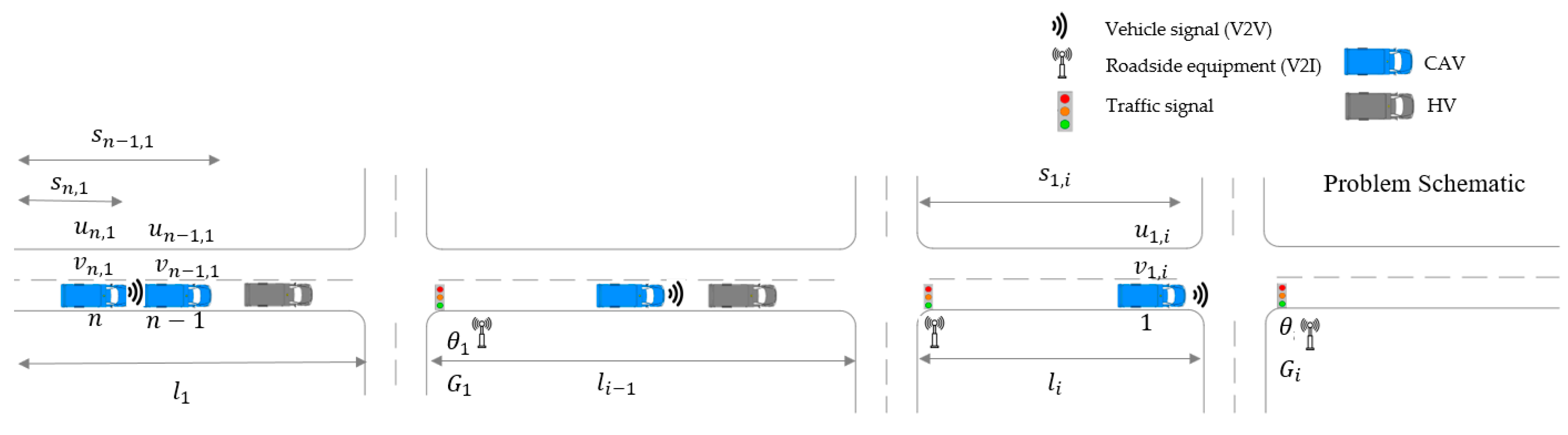
The problem aims to control the microscopic longitudinal behaviors of CAVs by minimizing the travel time given a fixed signal timing on an urban signalized arterial corridor. As shown in Figure 1, the mixed traffic travels through consecutive intersections on the urban street from upstream intersection 1 to intersection $i$ at downstream. The traffic is a mixture of HVs and CAVs. Communication devices are installed on CAVs to ensure real-time information exchange via V2V and V2I.

The assumptions of the paper are listed as follows. The V2V communication is assumed to be active once a vehicle entering the block. Information related to the timing plan such as offset ${\theta }_i$, the duration of green $G_i$, green elapse time $G_{n,i}$, and geometrical variable block length $l_i$ can be received by CAVs with no delay. The overtaking behavior of a vehicle is not in the scope of concerns. The car following behaviors of HVs are assumed as known, and HVs slow down and stop in front of a signal when they cannot pass within the current green interval.

In Figure 1, the vehicles move forward in their longitudinal direction. The travel time of a vehicle within a block is defined as the duration between the time instant when it passes the intersection $i-1$ and the time instant it passes intersection $i$.

The vehicle dynamics within a block for a CAV are expressed by a state-space representation, indexed by the number of vehicles and intersections. On an urban street, the vehicles are not allowed to move backward. A CAV can obtain information of vehicle status such as position, acceleration, and speed from the preceding vehicle, no matter whether the preceding vehicle is a CAV or an HV.

The research question is how to reduce the travel time for all vehicles when they are traveling from the first intersection to the final intersection and provide a suitable trajectory for each vehicle. The difficulties of this problem are that traffic signals exist along consecutive intersections, cutting off the traffic. Multiple states exist for a vehicle, in which varying control horizons can appear; HVs are uncontrolled, and HVs and CAVs are mixed with arbitrary sequences, so an integrated centralized optimization is not applicable. In addition, the control horizon for each vehicle is different.

3. Methodology

The longitudinal control for CAVs follows a hierarchical structure: at the upper level, the travel time is calculated; at the lower level, the optimal control is applied to generate the trajectories.

3.1. Lower-Level Control: Mathematical Formulation of Optimal Control

When an individual vehicle is traveling within one block between two intersections, its state including position and speed is known. The problem is decomposed into different scenarios and is then scaled towards multiple vehicles along consecutive intersections. The constraints from the longitudinal position and feasible arrival moments of a vehicle with the presence of signals are mathematically described. Each scenario is explained with their transportation meaning and provided a solution of minimum travel time and trajectory.

As a solution for individual vehicles, the trajectory generates in an optimal control fashion. The state $x_{n,i}$ of a vehicle $n$ in intersection $i$ is defined as a combination of its longitudinal position $s_{n,i}$ within this block $i$ and longitude speed $v_{n,i}$:

$$x_{n,i}={\left(s_{n,i},v_{n,i}\right)}^T$$

(1)

The system writes with a linear time-invariant system (LTI):

$$x_{n,i}\left(t\right)=A{x}_{n,i}\left(t\right)+B{u}_{n,i}\left(t\right),$$

(2)

$$\mathrm{A}=\left[\begin{array}{cc}0& 1\\ 0& 0\end{array}\right]\mathrm{B}=\left[\begin{array}{c}0\\ 1\end{array}\right],$$

(3)

where the control variable $u_{n,i}$ is the acceleration of the vehicle. The cost function to ensure optimal performances is defined as follows considering the comfort and terminal performances:

$$J_{n,i}=\min {{\displaystyle \int }}_{t=0}^{T_{n,i}}L\left(x_{n,i}\left(t\right),u_{n,i}\left(t\right)\right)dt+\mathsf{\Phi }\left(T_{n,i},x_{n,i}\left(T_{n,i}\right)\right),$$

(4)

where the ending time or the control horizon $T_{n,i}$ is a variable which is determined systematically. It is then discussed in Section 3.2, based on different scenarios. The running cost is set as an instantaneous cost showing the penalties concerning comfort. It is expressed as the quadratic term of acceleration:

$$L=\frac{1}{2}{u}_{n,i}{}^2.$$

(5)

The terminal cost gives penalties so that the final states can approach desired values (terminal speed and terminal distance):

$$\mathsf{\Phi }=w_1{\left(x_{n,i}{}^{\left(1\right)}\left(T_{n,i}\right)-l^{*}{}_{n,i}\right)}^2+w_2{\left(x_{n,i}{}^{\left(2\right)}\left(T_{n,i}\right)-v^{*}{}_{n,i}\right)}^2.$$

(6)

Again, $T_{k,i}$ will be determined systematically. Weighing factors $w_1$ and $w_2$ show the penalty for the state deviation from the terminal speed and the terminal distance at the end of the horizon. The desired speed is set to the terminal speed at each intersection for each vehicle: $v^{*}{}_{n,i}=v_0$. The block length between two intersections is used as terminal distance $l^{*}{}_{n,i}=l_i$. The problem then writes:

$$J_{n,i}={\displaystyle \sum }_{K=1}^T\left({u_{n,i}}_{t+k-1}{}^2\right)+w_1\left({{x_{n,i}}^{\left(2\right)}}_T{}^2-2{{x_{n,i}}^{\left(2\right)}}_T{v}_{n,i}{}^{*}+v_{n,i}{}^{*2}\right)+w_2\left({{x_{n,i}}^{\left(1\right)}}_T{}^2-2{{x_{n,i}}^{\left(1\right)}}_T{l}^{*}+l_{n,i}{}^{*2}\right),$$

(7)

s.t.

$$\left(x_{n,i},u_{n,i}\right)\in \Omega {{\displaystyle \cap }}^{ }U,$$

(8)

where $\Omega$ represents the constraints from vehicle dynamics, including the limitation from maximal speed, maximal acceleration, distance, etc. $U$ represents the physical constraints from the preceding vehicle during the period when it follows preceding vehicle $f_{n,i}$.

$$\Omega =\left\{{x_{n,i}}_{t+1}=A_d{x_{n,i}}_t+B_d{u_{n,i}}_t,{u_{n,i}}_t\in \left(u_{n,i,lb},u_{n,i,ub}\right),x_{n,i}{}^{\left(1\right)}\in \left(0,l_i\right),x_{n,i}{}^{\left(2\right)}\in \left(v_{n,i,lb},v_{n,i,ub}\right)\right\},$$

(9)

$$U=\left\{s_{n,i}\le s_{n-1,i}+d_s+d_v,t\in \left(0, f_{n,i}\right)\right\},$$

(10)

where $d_s$ is a safe distance that can ensure safety, and $d_v$ is the vehicle length; $f_{n,i}$ is the duration of following, determined differently in different scenarios in upper-level control.

3.2. Upper-Level Control: Determination of Travel Time

Having set the variable horizon optimal control, the horizon $T_{n,i}$ is to be determined systematically. Some prerequisites are provided.

3.2.1. Following Behavior along Consecutive Signalized Intersections

With the availability of V2I techniques, CAV receives signal information including current state and future time phases such as $G_i$ and ${\theta }_i.$ The arrival moments should be in a feasible region (the collection of green) and the physical constraints should always hold for safety concerns. To avoid stopping, for CAVs, the set of feasible arrival moments $M_{n,i}$ should be in the collection of green time $G$:

$$M_{n,i}\in \left[{\theta }_i+C\ast \left(k-1\right),{\theta }_i+G_i+C\ast \left(k-1\right)\right],$$

(11)

where $C$ is the cycle length. If no preceding vehicle exists, $k$ is the counter of the cycles after the current cycle in which the vehicle can pass. $k^{*}$ is the optimal $k$ that minimizes the travel time. If a vehicle is not able to pass within this cycle, it is natural that it passes at the next cycle, only if the preceding vehicle has passed. Generally, k could be 0 or 1 showing whether a vehicle is able to pass at this cycle or the next:

$$k^{*}=agrmin{T}_{n,i}.$$

(12)

Accumulative position $p_{n,i}\left(t\right)$ of a vehicle $n$ at time $t$ can be denoted as the addition of two parts: the accumulative position along previous blocks from $1$ to $i-1$, and the current position $p_{n,i}\left(t\right)$ in this block $i$ for vehicle $n$ is:

$$p_{n,i}\left(t\right)={{\displaystyle \sum }}_1^{i-1}{s}_{n,i}+s_{n,i}\left(t-{{\displaystyle \sum }}_1^{i-1}{T}_{n,i}\right).$$

(13)

At time $t$, the vehicle has two state conditions which is either passed block $i$ or not. When the subject vehicle has a preceding vehicle in the same block, an inequality describes the situation:

$${{\displaystyle \sum }}_{i-1}{l}_i<p_{n,i}\left(t\right)<p_{n-1,i}\left(t\right)<{{\displaystyle \sum }}_i{l}_i.$$

(14)

Similarly, when the preceding vehicle is not in the same block, an inequality writes:

$${{\displaystyle \sum }}_{i-1}{l}_i<p_{n,i}\left(t\right)<{{\displaystyle \sum }}_i{l}_i<p_{n-1,i}\left(t\right).$$

(15)

If the subject vehicle has a preceding vehicle in the same block, its duration is constrained by the preceding vehicle. The moments that enter or leaves a block can be calculated from the values of accumulated travel time:

$$M_{n,i}={{\displaystyle \sum }}_1^{i-1}{T}_{n,i}, M_{n,i+1}={{\displaystyle \sum }}_1^i{T}_{n,i}.$$

(16)

When a vehicle has a preceding vehicle,$f_{n,i}$ stands for the time duration that the subject CAV following its preceding vehicle within this block. This duration is the subtraction of the moment the preceding vehicle leaves this block and the moment when the subject vehicle enters the block:

$$f_{n,i}=M_{n-1,i+1}-M_{n,i}.$$

(17)

To scale the problem to consecutive intersections, $G_{n,i}$ shows the duration of green before the vehicle passes the intersection at the moment $M_{n,i}$. This variable links the time of trajectories between two intersections.

3.2.2. Scenario Development

The continuation of position and speed are addressed by introducing variables such as the cycle length $C$, green time $G_i$, green elapse time $G_{n,i}$, and offset ${\theta }_i$. Each vehicle is planned only once in a block, the moment a vehicle passes the previous intersection becomes the starting moment the vehicle enters the next intersection; the information is indicated with the help of green elapse time. The final status of a vehicle becomes the initial status in the next.

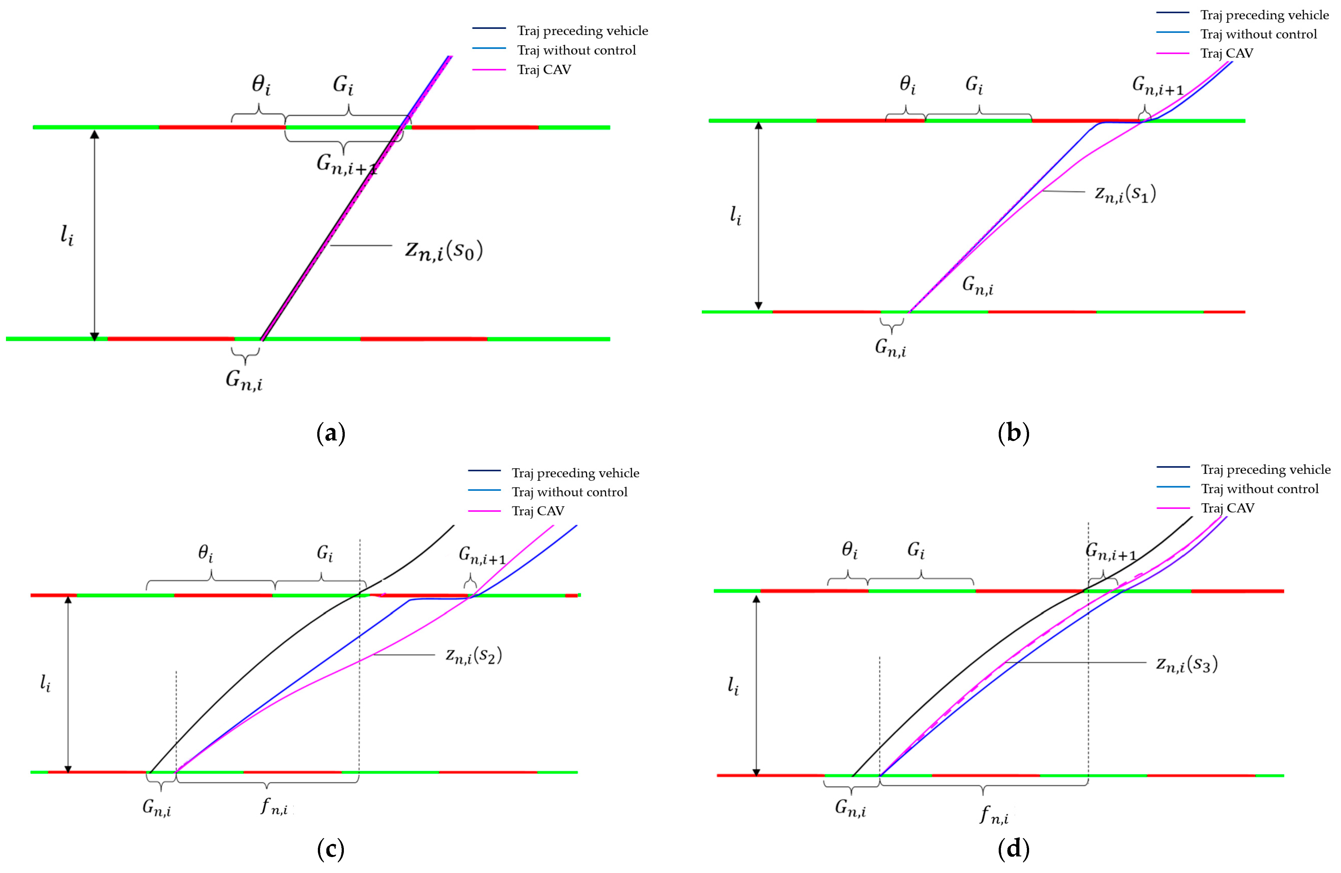
For CAVs, the arrival moments at the stop line of each intersection are estimated ahead. For HVs, the arrival moments are estimated using travel time estimation methods. According to the categories of the estimated arrival moments and whether there is a preceding vehicle, four scenarios can be defined, and they are noted as scenario 0, scenario 1, scenario 2, and scenario 3, respectively:

$$0<s_{n,i}\left(t\right)<l_i<s_{n-1,i}\left(t\right);M_{n,i}\in \left[{\theta }_i+C\ast \left(k-1\right),{\theta }_i+G_i+C\ast \left(k-1\right)\right],k\le 1,$$

(18)

$$0\le s_{n,i}\left(t\right)<s_{n-1,i}\left(t\right)\le l_i;M_{n,i}\in \left[{\theta }_i+C\ast \left(k-1\right),{\theta }_i+G_i+C\ast \left(k-1\right)\right],k>1,$$

(19)

$$0\le s_{n,i}\left(t\right)<s_{n-1,i}\left(t\right)\le l_i;M_{n,i}\in \left[{\theta }_i+C\ast \left(k-1\right),{\theta }_i+G_i+C\ast \left(k-1\right)\right],k>1,$$

(20)

$$0<s_{n,i}\left(t\right)<l_i<s_{n-1,i}\left(t\right);M_{n,i}\in \left[{\theta }_i+C\ast \left(k-1\right),{\theta }_i+G_i+C\ast \left(k-1\right)\right],k\le 1.$$

(21)

When the subject CAV is the leading vehicle in the same block, the way to minimize travel time is to accelerate and maintain its desired speed to travel through the block to pass the intersection (setting the speed limit as the desired speed $v_0$). The minimal travel time is obtained when the subject CAV accelerates to the desired speed and maintains the speed until it passes the signal ahead:

$$T^{*}{}_{n,i}=\left\{T_{n,i}\left|\right(u=u_0|v\le v_0),(u=0|v=v_0)\right\}.$$

(22)

The value of $G_{n,i+1}$ in the next intersection $i+1$ is calculated using travel time $T_{n,i}$ and the value of $G_{n,i}$, ${\theta }_i$ from the last intersection:

$$G_{n,i+1}=G_{n,i}+T_{n,i}-{\theta }_i.$$

(23)

For the subject CAV with no preceding vehicle in the same block, when it is not expected to pass the intersection within this cycle, it is planned to pass during the green in the next cycle, ($M_{n,i}\in \left[{\theta }_i+C\ast \left(k-1\right),{\theta }_i+G_i+C\ast \left(k-1\right)\right],k>1$), via a smooth path without stopping. The corresponding $T^{*}{}_{n,i}$ for both scenario 1 is calculated by:

$$T^{*}{}_{n,i}={\theta }_i+C\ast k^{*}-G_{n,i}+G_{n,i+1}.$$

(24)

$G_{n,i+1}$ varies the arrival moments, which is set as small as possible so that the startup time can be saved compared to human driving behavior.

For scenario 2, the calculation of $T^{*}{}_{n,i}$ and $G_{n,i+1}$ is the same as that of scenario 1. The difference is the subject vehicle has constraints from its preceding vehicle for the preceding vehicle is in the same block. $U$ is active as the physical constraints of the optimal control.

Scenario 3 shows when the subject CAV follows a preceding vehicle in this intersection, and it passes within the same green window as the preceding vehicle:$M_{n,i}\in \left[{\theta }_i+C\ast \left(k-1\right),{\theta }_i+G_i+C\ast \left(k-1\right)\right],k\le 1$. The corresponding $T^{*}{}_{n,i}$ is then calculated from:

$$T^{*}{}_{n,i}=max(T_{n-1,i}-f_{n,i}+t_{0,i},\frac{l_i}{v_0}).$$

(25)

$$G_{n,i+1}=G_{n,i}+T_{n,i}-{\theta }_i-C\ast k^{*}.$$

(26)

Note that the minimal travel time cannot be smaller than the value when the vehicle is traveling with the desired speed (in that case, the travel time from scenario 3 is no smaller than that from scenario 0). $U$ is active as the physical constraints from the preceding vehicle.

Although an HV cannot respond to a CAV, a CAV can detect the position of its preceding HV. An estimation of the HV’s travel time is conducted. The desired headway $t_{0,i}$ when a CAV following an HV is set to be larger than that an HV follows an HV to ensure safety. The travel time when a CAV follows an HV is calculated as:

$$T^{*}{}_{n,i}=max(T_{n-1,i}-f_{n,i}+t_{0,i\left(HV\right)},\frac{l_i}{v_0}).$$

(27)

An HV is expected to slow down and stop if it cannot pass an intersection within the green duration. They will be modeled remaining at a standstill at the stop bars during the red phases. The subject CAV does not need to follow closely to an HV. Instead, it passes with a smooth trajectory without stopping. The calculations of $T^{*}{}_{n,i}$ and $G_{n,i+1}$ are the same as the case when it follows a CAV. In the schematic diagrams of Figure 2, the blue line shows the estimated trajectory of an HV, and a black line shows the preceding vehicle trajectory. A magenta line represents the trajectory of a CAV.

3.3. Synthesized Algorithm

In lower-level control, the optimal control has been set up for each vehicle to calculate their optimal trajectories. In upper-level control, the scenarios are developed. In each scenario, the way to find the minimum travel time has been introduced. The problem in this paper is to minimize the total travel time for all vehicles therefore the hierarchical control is addressed systematically in a synthesized way.

According to the analysis of scenarios, scenario 0 is designed as the vehicle that can drive with its speed limit. Scenario 3 follows preceding vehicle successfully without being hampered by a red light. Both scenarios are with no time loss. Scenario 1 and 2 experienced time losses at red. It is obvious that, at the same intersection $i$, the travel time for each scenario has the following relations:

$$T^{*}{}_{n,i}\left(scnario 0\right)<T^{*}{}_{n,i}\left(scnario 3\right)\le T^{*}{}_{n,i}\left(scnario 1\right)\le T^{*}{}_{n,i}\left(scnario 2\right).$$

(28)

Apparently, the travel time reaches minimal when an ideal condition can occur in which all scenarios are scenario 0. Nevertheless, a vehicle may not be able to drive with scenario 0 along all the blocks. In this case, replacing one of the scenarios into another scenario with the least cost for vehicle $n$ achieves the minimal costs that are feasible. Therefore, a greedy heuristic is to try to plan scenario 0 or scenario 3 first, and then to plan scenario 1 or 2.

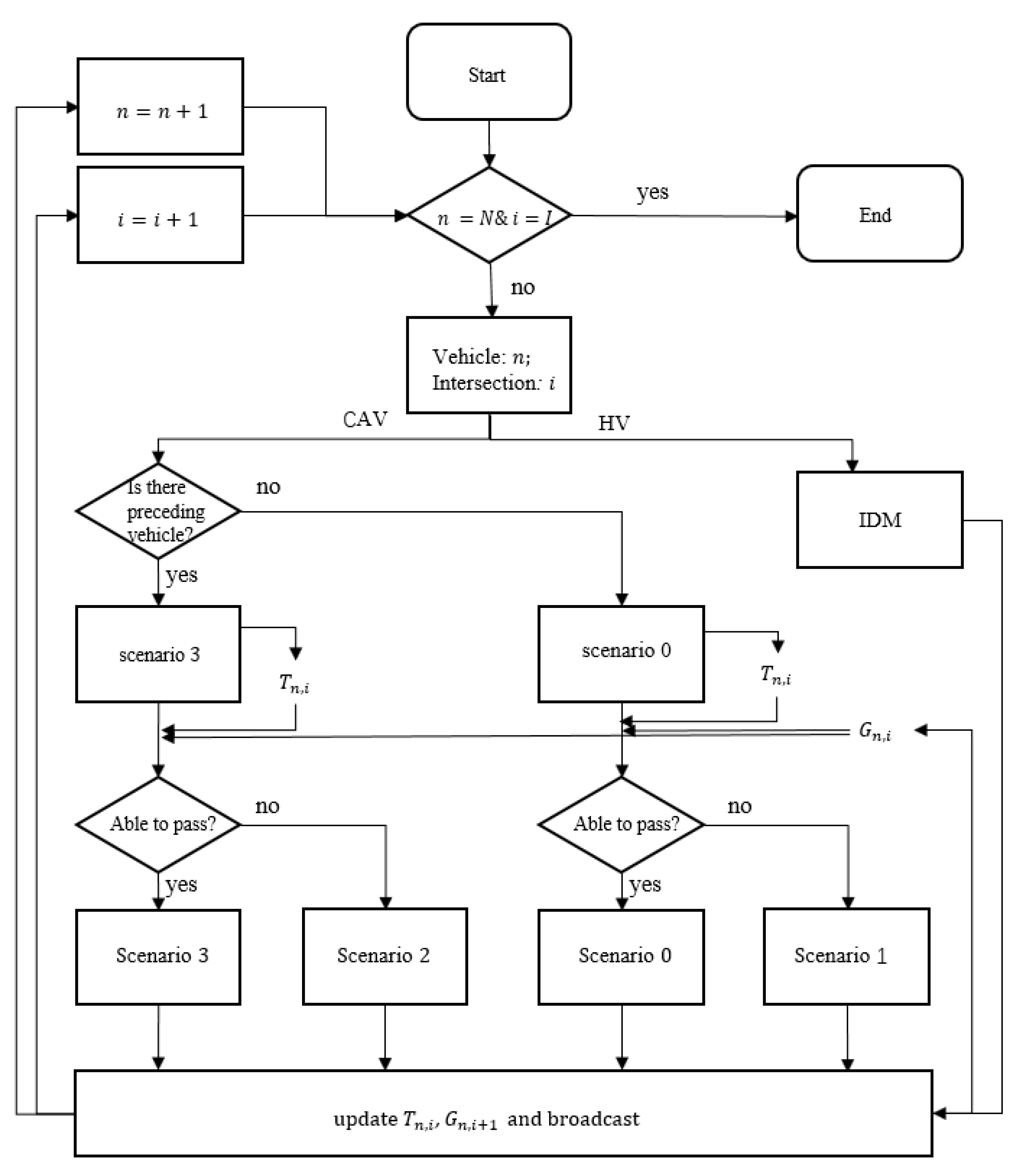
Define $z_{n,i}\triangleq {[u_{n,i}{\left(0\right)}^T,\dots ,u_{n,i}{\left(t-1\right)}^T]}^T$ as the decision variable of vehicle $n$ from the time instant 0 to $t$ in each intersection $i$. Once a selection of scenarios is made, the minimal travel time $T_{n,i}{}^{*}$ is calculated. The decision variables of the preceding vehicle ${\overline{z}}_{n-1,i}$ and the constraints inputs into the next calculation. By assuming there are $N$ vehicles and $I$ intersections, the calculation process is listed as follows:

Start: start with intersection $i=1,n=1$

• Step 1: If $0\le s_{n,i}\left(t\right)<s_{n-1,i}\left(t\right)\le l_i$, go to Step 2a; otherwise, go to Step 3a.
• Step 2a: $M_{n,i}\in \left[{\theta }_i+C\ast \left(k-1\right),{\theta }_i+G_i+C\ast \left(k-1\right)\right],k=1$, obtain the numerical solution as scenario 0; otherwise, go to Step 2b.
• Step 2b: $M_{n,i}\in \left[{\theta }_i+C\ast \left(k-1\right),{\theta }_i+G_i+C\ast \left(k-1\right)\right],k>1$, obtain the numerical solution for optimal control problem as scenario 1.
• Step 3a: $M_{n,i}\in \left[{\theta }_i+C\ast \left(k-1\right),{\theta }_i+G_i+C\ast \left(k-1\right)\right],k=1$, obtain the numerical solution for optimal control problem as scenario 3; otherwise, go to Step 3b.
• Step 3b: $M_{n,i}\in \left[{\theta }_i+C\ast \left(k-1\right),{\theta }_i+G_i+C\ast \left(k-1\right)\right],k>1$, obtain the numerical solution for optimal control problem as scenario 2 (following a CAV) or scenario 3 (following an HV).
• Step 4: Find the solution $z_{n,i}{}^{*}$ for vehicle $n$ at intersection $i$ and broadcast all the outputs from current plan to all other CAVs. The known decision variables are ${\overline{z}}_{n-1,i}$ then.

End: End by $i=I, n=N$.

As described in the algorithm, the controller determines each CAV individually and broadcasts its information and solutions. Information is broadcasted to the follower if it is a CAV. This proceeds until all the vehicles have solutions for trajectory profiles. The process is demonstrated in Figure 3.

4. Numerical Simulations

The proposed method was implemented in MATLAB, and the numerical simulations are demonstrated below. To test conditions under light traffic does not have much value since no traffic backpropagation will happen, so only the cases with moderate demands were considered. Two cases were presented to validate the method. Case 1 compared the method with the situation when all vehicles were HVs. HVs were assumed to slow down and stop when approaching a signalized intersection if they expected to fail to pass and remain standstill at the stop bars during the red phases. HVs were assumed to follow preceding vehicles using the intelligent driver model (IDM) model [45]. Case 2 compared the proposed method with a benchmark when all CAVs drive smoothly to avoid stopping at intersections without the consideration of minimal travel time.

Both cases comprised two examples. In one example, the initial average headway input was set as 5 s. In the other example, the initial input headway was 3 s. The desired headway for a CAV and the IDM model was set as 3 s; the desired headway for a CAV following an HV was set at 4 s for safety concerns. Multiple runs with random seeds were applied in each case to calculate the average travel time savings under each penetration rate. The parameters used in the experiment are listed in

Table 1. Values of parameters in the experiments.

Parameters	Notation	Value
Block length $\left(\mathrm{m}\right)$	${\mathrm{l}}_{\mathrm{i}}$	1000
Number of blocks	N	3
Number of vehicles	I	60
Cycle length (s)	$\mathrm{C}$	100
Green duration (s)	${\mathrm{G}}_{\mathrm{i}}$	60
Offset (s)	${\mathsf{\theta }}_{\mathrm{i}}$	30
Weight for terminal distance	${\mathrm{w}}_1$	10
Weight for terminal speed	${\mathrm{w}}_2$	10
Number of vehicle inputs	N	60
Safe distance (meter)	${\mathrm{d}}_{\mathrm{s}}$	5
Vehicle length (meter)	${\mathrm{d}}_{\mathrm{v}}$	5
Desire headway (s)	${\mathrm{t}}_{0,\mathrm{i}}$	3
Desire headway a CAV following an HV (s)	${\mathrm{t}}_{0,\mathrm{i}\left(\mathrm{HV}\right)}$	4
Maximum speed (m/s)	${\mathrm{v}}_{\mathrm{n},\mathrm{i},\mathrm{ub}}$	20
Minimal speed $(\mathrm{m}/\mathrm{s}$)	${\mathrm{v}}_{\mathrm{n},\mathrm{i},\mathrm{lb}}$	5
Maximum acceleration $(\mathrm{m}/{\mathrm{s}}^2$)	${\mathrm{u}}_{\mathrm{n},\mathrm{i},\mathrm{ub}}$	2
Minimal deacceleration $(\mathrm{m}/{\mathrm{s}}^2$)	${\mathrm{u}}_{\mathrm{n},\mathrm{i},\mathrm{lb}}$	−2

.

4.1. Performance under Different Penetration of CAVs

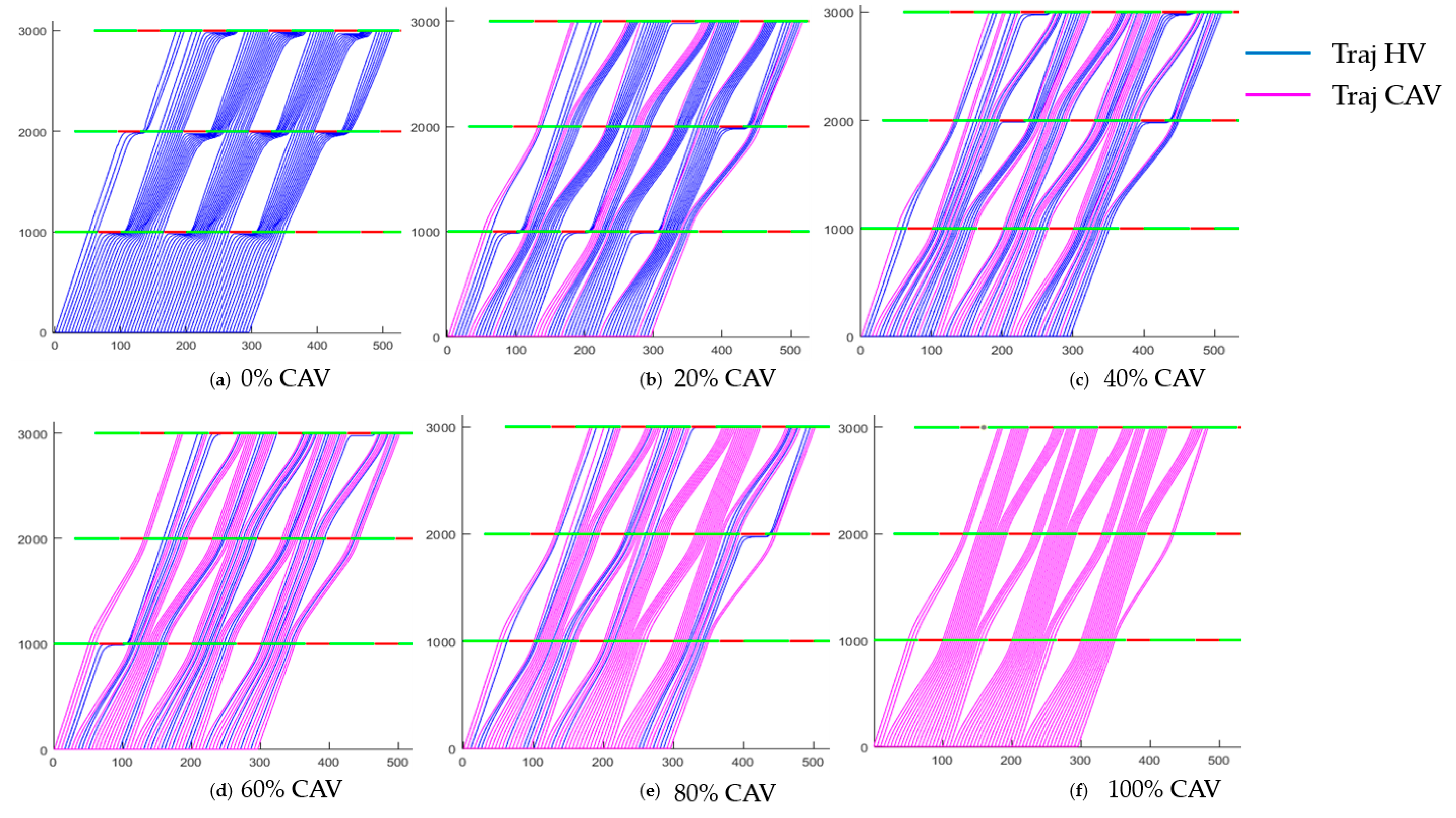
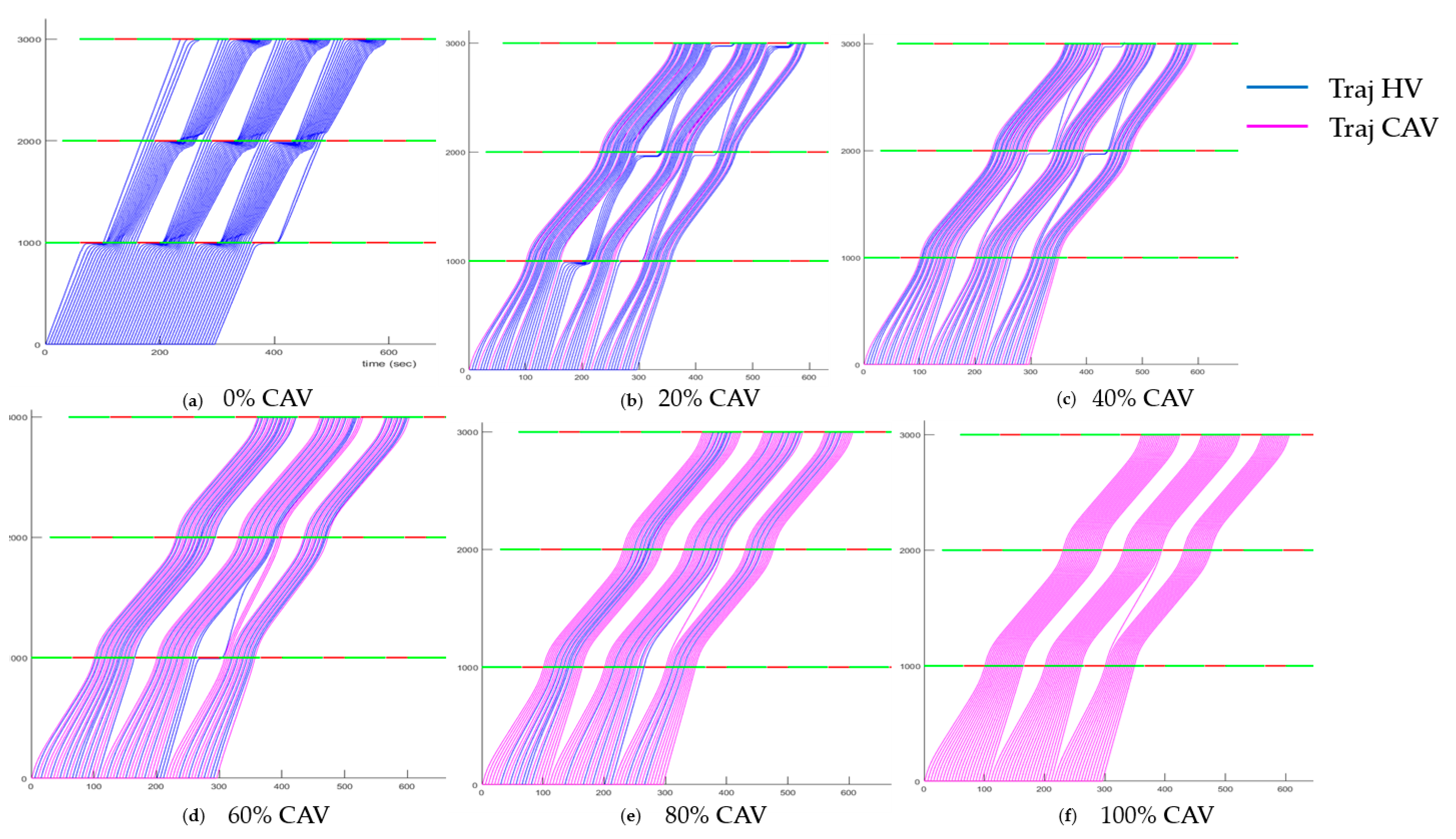
Case 1 compares the results when no CAVs and when some CAVs using the proposed are applied. The simulated results are presented in Figure 4 and Figure 5.

When the initial headway for CAVs was 5 s, the CAVs trajectories could lead the whole platoon to decompose and reconstruct reasonably. This led to a reduction in travel time in the first step. The results also showed that the proposed method can reduce the number of stops; as a result, the queues and backpropagation shockwaves were mitigated to reduce the startup time, which saved travel time in the second step. The method compressed the headways for CAVs when the initial headway was larger than the desired headway, which made the traffic stream compact, leading to a reduction of travel time in the third step. Compared to the situations when all vehicles are HVs (0%), the effects of mitigation of adverse phenomena became more significant with the increase of penetration rates. When the penetration rate was 100%, the stops were mostly eliminated, and no queue and backpropagation shockwave showed.

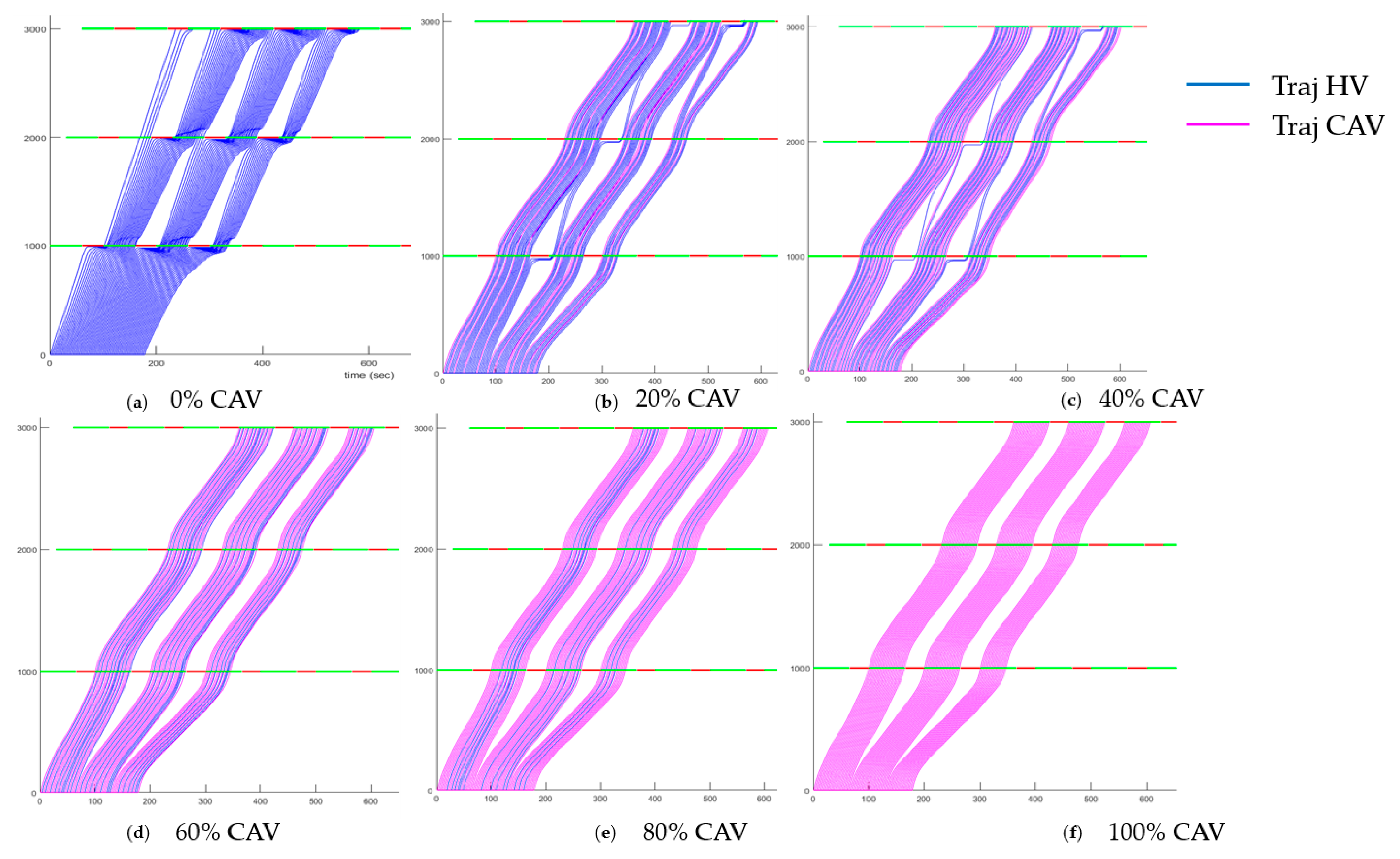
When traffic demand was higher, according to Figure 5, although the initial headways were so small that they cannot be compressed, travel time was saved from the first two steps: The whole platoon still decomposed and reconstructed in a certain manner to ensure vehicles could pass with the shortest time, and the queues and backpropagation shockwaves were also mitigated. 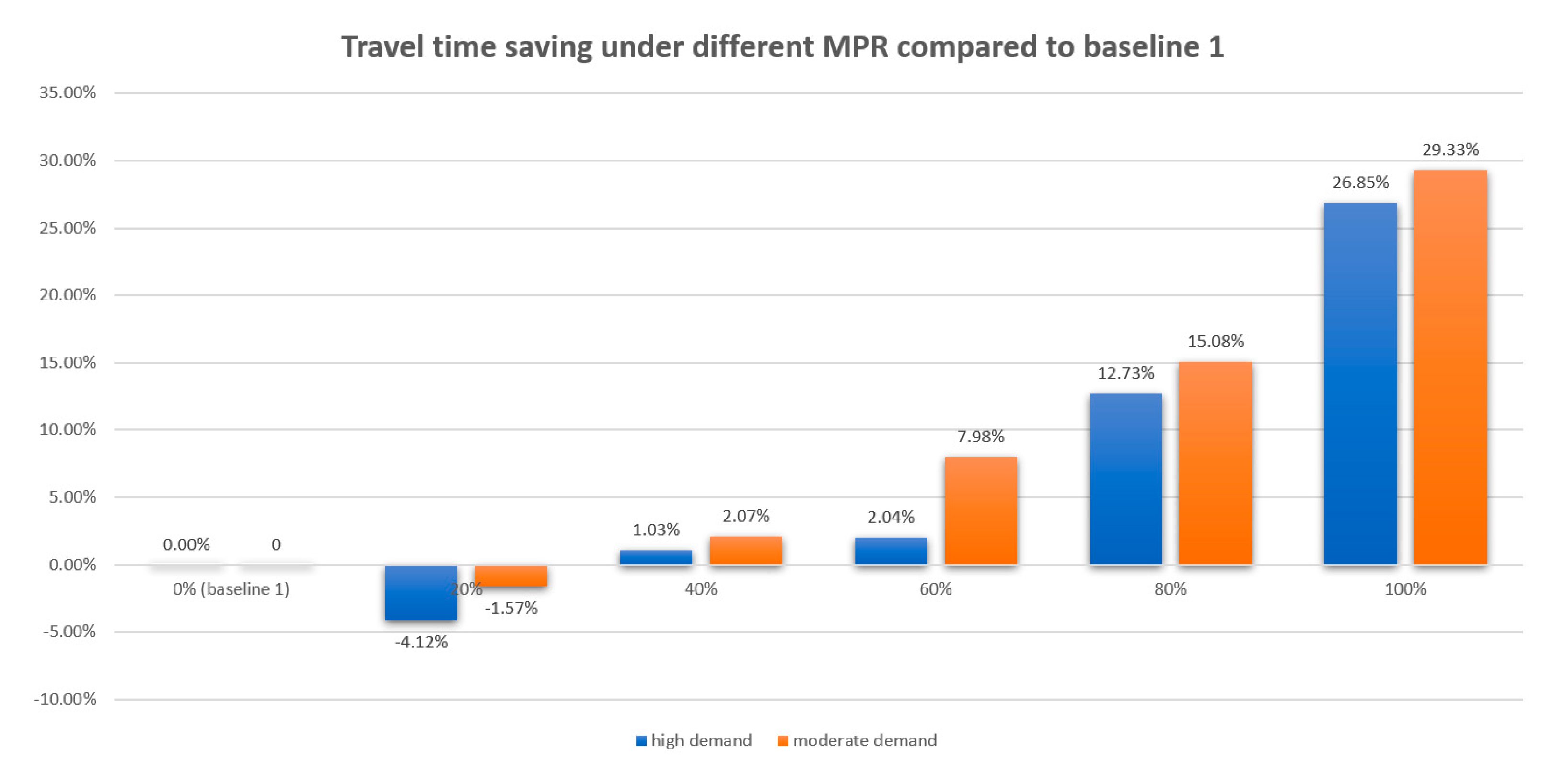The overall results after multiple runs are presented in Figure 6.

When the penetration rate of CAVs was as low as 20%, the methods could lead to a negative effect (−1.57% and −4.12 %). The reason was that a large desire headway (4 s) for a CAV following an HV was set to ensure safety, which was larger than the case when a CAV followed a CAV (3 s) or when an HV followed an HV (3 s). However, with the increasing penetration rates of CAVs, the travel time savings become effective. The travel time savings were significant when the penetration rate was larger than 60% for both cases. When a full penetration rate was assumed, the proposed method can provide travel time savings of 29.33 % and 26.85 % in two examples.

4.2. Compare with a Benchmark

A benchmark was configured with the following settings: (1) the trajectories of HVs were generated in the same way as in case 1; (2) the trajectories of CAVs were generated based on a benchmark. For case 2, only the optimal control was used to smooth the trajectories of the leading CAV at an intersection, and the others followed their leaders. Similarly, in these cases, different initial headways were demonstrated.

As seen in Figure 7 and Figure 8, although smooth trajectories could reduce travel time by reducing time-consuming stop and startup driving behaviors at an intersection, they led to an increase in travel time if multiple intersections were involved and the local minimal travel time was not considered. This case showed the importance of the proposed method to calculate the minimal travel time locally under all possible scenarios.

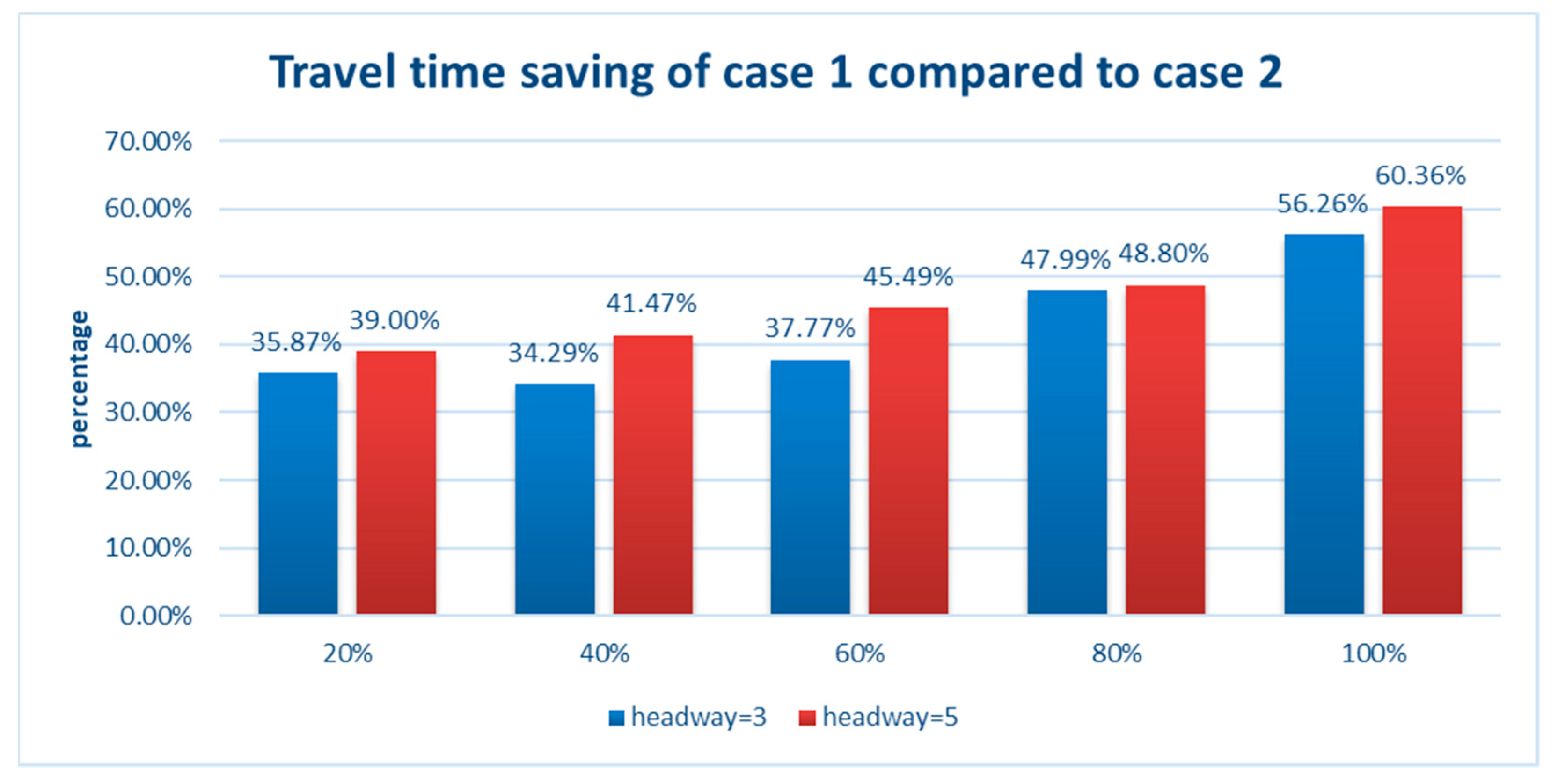
The outputs from case 1 and case 2 showed a significant difference in Figure 9.

Comparing case 1 (using the proposed method to control CAVs) with case 2 (using a benchmark), 35.87% (shorter headway) and 39.00% (larger headway) travel time savings were shown, even when the penetration rate was as low as 20%. The percentage increased to 56.26% and 60.36% when a full penetration rate was assumed.

5. Conclusions

Traffic oscillation and queue backpropagation caused by traffic signals can interrupt traffic streams periodically and increase the travel time for drivers. To ensure sustainable transport on a signalized urban street by improving mobility, a connected automated vehicle hierarchical longitudinal control for mixed traffic on consecutive signalized arterials was proposed to control multiple vehicles along multiple intersections, considering their varying control horizons. The main aim is to focus on vehicle mobility on signalized arterials to improve sustainable urban transportation.

In the lower-level layer, mathematical formulations were developed for the relations between vehicles and signals during the time vehicles were traveling along consecutive signalized intersections. In the upper-level layer, the conditions of vehicles are decomposed into four scenarios. In each scenario, a minimal travel time is calculated. A synthesized algorithm is used to connect lower-level and upper-level layers.

Two cases were developed to validate the proposed control strategy. Case 1 concerned a non-CAV setting and Case 2 assumed all CAVs with smooth trajectory without considering the travel time. The proposed method significantly reduced the number of stops. When it came to travel time savings, when the initial headway was larger, the travel time saving ranged from −1.57% to 29.33 %. When the initial headway was smaller, the travel time saving was also significant (ranging from −4.12 % to 26.85 %). Compared to case 2 using a benchmark, the proposed method can save travel time from 35.87% to 56.26% and 39.00% to 60.36%.

The limitation of this paper was that the status of the CAVs and HVs were assumed as deterministic, and only a single lane was considered in the problem. In the future, how these scenarios are stably switched in the real world will be considered. In addition, the method is to be generalized to multilane scenarios by considering lane changing and overtaking behaviors.