Seawater Desalination via Waste Heat Recovery from Generator of Wind Turbines: How Economical Is It to Use a Hybrid HDH-RO Unit?

Abstract

Over recent years, the concept of waste heat recovery from the generators of wind turbines for driving a thermal-driven desalination system was introduced, and its advantages were highlighted. However, any selection of a bottoming thermal-driven desalination system among different existing technologies should be taken under consideration before making an ultimate recommendation. Unfortunately, no comprehensive comparison is available in the literature to compare the performance as well as the cost aspects of using the waste thermal energy of the generator of a wind turbine for desalinating seawater, comparing them with those of a layout where the power of the wind turbine is directly supplied to a mechanically driven desalination system for the same amount of drinkable water production. This study aims at analyzing the economic aspects of waste heat recovery from the generators of wind turbines for seawater desalination via the humidification-dehumidification (HDH) approach, versus the reverse osmosis (RO) unit. For this purpose, a closed-air water-heater HDH unit, directly coupled with a RO unit (called a hybrid HDH-RO unit) is employed, in which thermal energy is provided by the heat dissipating from the generator of the wind turbine while its power is supplied directly by the wind turbine. The energetic and exergetic performance, along with the cost aspects of a hybrid HDH-RO unit driven by the wind turbine, are compared with those of a solo RO unit. The results of the study were extended for six different types of wind turbines, and we concluded that the unit cost associated with the freshwater produced by the waste heat recovery approach is astronomically higher than that of the solo RO system for all wind turbine models, and hence is not practically feasible. It was found that more power can be recovered from the discarded brine from the solo RO unit than the hybrid HDH-RO unit. In addition, the solo RO desalination system, working directly with the power of the wind turbine, has a less complex configuration, and hence its investment cost rate is significantly lower than that needed for setting up an HDH-RO unit. At high wind speeds, however, the cost penalty associated with the freshwater produced by the HDH-RO unit decreases, but it is still huge. Among all screened wind turbines, the GW-136/4.8 is most appealing in terms of greater power generation, but its investment cost rate is the highest among all models due to its high rated power value. However, the freshwater unit cost of the GW-136/4.8 is significantly lower than the values obtained for other models. Finally, the two locations of Manjil and Zabol are selected as a benchmark and the results of the simulation are extended for these locations.

1. Introduction

A desperate need for large-scale power supply from available or developing prime movers has been recognized as one of the top solutions to tackling power shortage or problems associated with its intermittency. One approach to building a monolithic power plant is to eliminate as much heat dissipation from different components or (in the case of the high-grade quality of this waste heat) to transmit this thermal heat to valuable by-products. By materializing such an idea, the energy conversion performance of the whole plant can be increased, extra or various by-products can be produced and stored, the unit cost associated with the main product as well as the by-product(s) can be decreased, and environmental issues arising from the deployment of this thermal heat into the surroundings can be ameliorated, to exemplify some of the benefits. Waste heat capturing from chemical/thermal processes in electrical, mechanical and petrochemical industries or plants has been discussed practically and employed in various sectors and industrial processes. Despite the widespread application of waste heat elimination via conventional processes and sources, less attention is paid to the idea of employing the same concept for recovering the heat dissipated from special sectors like the wind turbines’ cooling unit. The concept behind this idea becomes enthralling once a wind farm is ahead of the engineers. Furthermore, with recent technological advances accomplished in the design and construction of gigantic wind turbines, one can expect to have a huge amount of invaluable thermal energy dissipating from a wind turbine.

In Europe, countries like Russia have started to increase their power generation capacity since 1990, but it was slow due to the slow growth of the industrial production volume [1]. Russia has a significant wind energy technical potential—more than 60 PWh of electricity per year [1]. The regions of the Russian north, and in particular the Gulf of Ob, the Kola Peninsula and most of the coastal strip of the far east, belong to the windiest zones of the world, according to the global classification. Power generation from wind farms in Russia is currently only 148 GWh [1].

Over the course of the last decade, several studies have turned the spotlight on versatile usage of the heat dissipating from the generator (or also the gearbox) of wind turbines, via recommending various approaches for cooling down the generator inside the hub (for capturing its dissipating heat) or also via proposing different thermal-driven energy systems (for transmitting this thermal heat into other forms). Although enlarging the unit capacity of the wind turbines can be regarded as one scheme to accelerate the cooling process of the generator, it significantly increases the insulation aging, due to the increase of the inductance coil load [2]. Meanwhile, although several studies have reported satisfactory results in the cooling process of the wind turbines’ generator via liquid circulation, due to its high maintenance, simple configuration, simple monitoring processing, and low investment cost [2,3], some results substantiate the installation of auxiliary ventilation equipment [4]. Khalilzadeh and Nezhad [5] used water for cooling down the generator of an Enercon-126 wind turbine, and used the obtained thermal heat for desalinating seawater by employing a thermal-driven multi-effect distillation (MED) unit. By assuming a generator with an efficiency of 93%, they calculated waste heat rates of 122 kW, 155.3 kW, 192.16 kW, 231 kW, and 269.9 kW, and freshwater rates of 0.99 m³/h, 1.26 m³/h, 1.56 m³/h, 1.88 m³/h, and 2.2 m³/h at wind speeds of 8 m/s, 9 m/s, 10 m/s, 11 m/s, and 12 m/s, respectively. In another study and also by using oil and water in a liquid-liquid-air cooling system, Khalilzadeh and Nezhad [6] used thermal heat from the same wind turbine for trigeneration using the following bottoming cycles: an organic Rankine cycle (ORC) for power generation, an absorption chiller for cooling generation, and a heating unit for heat generation. They introduced the recovery heat exchanger (used for transferring waste heat of the wind turbine to the bottoming cycle) as the component with the highest exergy destruction, accounting for around 75% of the total exergy destruction rate. In 2014, De Risi et al. [7] recommended the use of a nanofluid (Al₂O₃/water) instead of pure water for enhancement of the cooling process, and later, in 2018, the idea was theoretically supported by Rostamzadeh and Rostami [8]. Accordingly, the authors used a humidification-dehumidification (HDH) desalination unit for converting the thermal waste of the wind turbine into freshwater and recommended a nanofluid of Cu/water instead of Al₂O₃/water. More recently, Rostamzadeh and Rostami [9] used an absorption chiller driven by the waste heat of an Enercon-70 wind turbine, and produced drinkable water and cooling for the two humid and windy regions of Kahak and Manjil in Iran. They also recommended the use of Cu/water nanofluid, and concluded that by increasing Cu concentration from 0.5% to 7%, the cooling capacity increases from 5.1 kW to 5.8 kW, the freshwater rate increases from 126.9 L/day to 144.5 L/day, and air supply increases from 9.27 m³/min to 10.56 m³/min.

Seawater desalination via renewable energy-based technologies is recognized as a viable solution to tackling the growing freshwater shortages in different spots of the globe. The feasibility of direct supply of the electrical power produced by a wind turbine to mechanical-driven desalination systems has previously been carried out and the advantages and obstacles they face have comprehensively been explained. Over the last few years, the concept of waste heat recovery from the generator of the wind turbines for driving a thermal-driven desalination system has been introduced, and its advantages highlighted. However, any selection of the bottoming thermal-driven desalination system among different existing technologies should be taken on board before proposing an ultimate recommendation. Unfortunately, no comprehensive comparison is available in the literature to compare the performance as well as the cost aspects of using waste thermal energy from the generator of a wind turbine for desalinating seawater with those of a layout where the power of the wind turbine is directly supplied to a mechanically driven desalination system for the same amount of drinkable water production.

Based on the reviewed open-source literature, it can be emphasized that capturing the waste heat of wind turbines via appropriate methods and using it for producing useful forms of energy can be regarded as a real demand. The need has previously been addressed by several authors, as reviewed in the previous paragraph. The current study aims at investigating the economic prospects of using the waste heat of the generator of various wind turbines for freshwater production instead of using a mechanically driven desalination system directly supplied by the power of a wind turbine. A reverse osmosis (RO) desalination system, driven by the power of the wind turbine, is considered as the reference system, while a hybrid HDH-RO desalination system driven by both waste heat and the power of the wind turbine is accounted for to understand the economic advantages/disadvantages of the new layout. Although the previous study has recommended the use of HDH driven by the waste heat of the generator of the wind turbine in terms of performance [8], no investigation of the economic aspects of the layout was discussed. Furthermore, the study conducted by Khalilzadeh and Nezhad [5] has not presented a comparison in terms of cost metrics between a thermal-driven MED unit and its power-driven counterpart (i.e., a MED-MVC (mechanical vapor compression) unit), and the authors have reported a relatively high freshwater cost of 23 $/m³. Although this cost is much lower than the value obtained through this study, the present investigation does not seek to scrutinize the appropriateness of employing an MED or HDH unit, since the scale and the approach accounted for regarding freshwater production by the two methods are completely different (and is out of the scope of the present study, although it will be accounted for in future studies).

In this study, as in our previous study [8], an HDH unit is used to capture the waste heat of the wind turbine’s generator for seawater desalination. Based on the results of our previous studies [8,9], Cu/water is used in the liquid-liquid cooling system of the wind turbine due to its exhibiting a high performance. The present study aims at producing more freshwater by consuming a specific portion of the power produced by the wind turbine in the desalination unit via hybridizing a RO unit with the HDH unit. That is to say, the waste brine stream exiting from the HDH unit is fed into a RO unit for more freshwater production. Due to the high salinity and temperature of the brine discarded from the HDH unit, one can surmise that, by employing the hybrid HDH-RO desalination unit, the performance of the RO unit increases while its operating cost decreases [10,11,12]. The superiorities and inferiorities of the devised layout versus the reference system (the RO unit driven by the mechanical power of the wind turbine by the direct supply of a seawater stream to the desalination unit) have comprehensively been discussed in terms of thermodynamics and thermoeconomics. Several studies have previously recommended the idea of supplying the required power of a RO unit from wind turbines in remote areas, like islands [13,14]. However, no comparison is made between these two approaches in these studies.

2. Description of Layout

The layouts of the reference system driven by direct supply of mechanical power supplied from the wind turbine and of the hybrid HDH-RO desalination unit driven by both thermal and mechanical energies of the wind turbine are displayed in Figure 1. Six different types of wind turbines are selected for this paper, in which the main geometrical and operating specifications of each case are listed in

Table 1. Main specifications of the screened wind turbines.

Wind Turbine Models	Rated Power (kW)	$\mathbf{Cut}-\mathbf{in} \mathbf{Wind} \mathbf{Speed} \left(\frac{\mathbf{m}}{\mathbf{s}}\right)$	$\mathbf{Rated} \mathbf{Wind} \mathbf{Speed} \left(\frac{\mathbf{m}}{\mathbf{s}}\right)$	$\mathbf{Cut}-\mathbf{Out} \mathbf{Wind} \mathbf{Speed} \left(\frac{\mathbf{m}}{\mathbf{s}}\right)$	$\mathbf{Swept} \mathbf{Area} ({\mathbf{m}}^2)$	Diameter (m)	Hub Height (m)
Enercon 101 E2 (E-101/3.5)	3500	2	15	25	8012	101	74
Vensys 115 (V-115/4.1)	4100	3	13.5	25	10,378	115	72.5
Gamesa 128 (G-128/4.5)	4500	1	12	27	12,868	128	81
Goldwind 136 (GW-136/4.8)	4800	2.5	11.2	26	14,526	136	86
Eno energy 114 (Eno-114/4.8)	4800	3	14	25	10,369	114.9	92
Adwen 5-116 (AD-5-116/5)	5000	4	12.5	25	10,568	116	92

. The reference system is actually a RO desalination unit driven by the mechanical power of the wind turbine. The layout in Figure 1a is selected as a reference system to quantitatively and qualitatively measure the amount of extra freshwater produced via waste heat recovery from the generator of the wind turbine, and also to compare the cost penalty associated with capturing waste heat from the generator of the wind turbine for the same purpose when an HDH-RO system is employed. In addition, several studies have previously recommended the idea of supplying the required power of a RO unit from wind turbines in remote areas, like islands [13,14]. However, the idea of running a hybrid desalination system with both the thermal and mechanical potential of wind turbines is not accounted for yet, and hence the superiorities and inferiorities of the layout can be discerned by comparing the main performance and cost metrics with those of the reference unit.

In the hybrid HDH-RO desalination unit, the nanofluid transfers the heat discarded from the generator of the wind turbine to the heater of the HDH unit through two separate loops. The reason behind the selection of this configuration for recovering the waste heat of the wind turbine is thoroughly explored in our previous study [9]. As the HDH unit receives this heat from the heater, the hot stream warms up the cold seawater stream flowing in from the dehumidifier and directs it towards a spray process occurring between seawater and the dry air inside the humidifier. Next, due to the high salinity and temperature of the brine exiting from the humidifier, this brine is recovered for further freshwater production by directing it towards an RO unit. The brine is first pressurized to a high-pressure state via a high-pressure pump (HPP) and then is passed through a permeator (membrane of the RO unit). Finally, the high saline brine pumping out from the permeator is directed into an energy recovery turbine (ERT) for extra power generation, due to its high pressure.

3. Selection and Description of Locations

Iran is located in the Middle East and is connected to the Caspian Sea in the north and the Persian Gulf and Sea of Oman in the south. The surface area of Iran is 1,648,195 km² (ranked as the second-largest in the Middle East and eighteenth in the world) [15]. Based on the Standardized Precipitation-Evapotranspiration Index (SPEI) reported every 10 years, the drought contour for Iran is illustrated in Figure 2. As Figure 2 shows, the majority of regions in Iran experience severe drought due to indiscriminate energy consumption, poor management, and more specifically, a lack of precipitation. The average precipitation is 250 mm/year which is significantly less than the global average (831 mm/year) [15]. In addition to the drought atlas, it is crucial to consider the wind atlas of Iran before selecting the case study locations for the devised hybrid desalination system’s working wind turbine. The wind atlas of Iran for a height of 100 m must be considered, since in the simulation a wind turbine with a GW-136/4.8 model and hub height of 86 m is selected (the nearest altitude to the height of the hub). Figure 3 displays the wind atlas of Iran. As Figure 3 indicates, the east of Iran has strong wind potential, while some parts in the north and northwest suffer from a lack of wind speed. In addition to the wind speed potential and drought, it is highly imperative to consider the seawater availability in the selection of the case study’s location, to provide ample seawater feed for the devised system. Considering all these factors on the ground, the two locations of Manjil and Zabol were chosen, to satisfy all factors simultaneously. The location of each city is presented in Figure 2 and Figure 3 with blue stars. Manjil is located in the north of Iran in the province of Gilan, at a distance of around 80 km from the Caspian Sea. The average wind speed of Manjil in the winter is 6 m/s (at an elevation of 40 m). Manjil experiences strong north winds with an average speed of approximately 14 m/s between May and September [16]. The average precipitation of Manjil is 216 mm/year, while the average precipitation of Gilan province is 1048 mm/year [17]. Zabol lies on the east of Iran and north of Sistan-Baloochestan province, and borders Afghanistan. Due to the dry and hot climate of Zabol, with long summers, the city suffers from a severe lack of drinkable water for most days of the year. The annually averaged wind speed of Zabol is about 7.5 m/s, where the wind intensity is high from April to October. In addition, the average precipitation of Zabol is about 70 mm/year, which is extremely low compared to that of the whole country (250 mm/year). Currently, Zabol is facing drinkable water shortages due to the lack of precipitation as well as the high salinity of groundwater. The geographical coordinates of the selected cities are presented in

Table 2. Geographical coordinates of selected cities.

City	Latitude	Longitude	Altitude (m)
Manjil	36°44′	49°24′	310
Zabol	31°01′	61°30′	485

.

4. Materials and Methods

4.1. Effective Thermophysical Properties of Nanofluid

The method behind the calculation of effective thermal and fluid properties of Cu/water nanofluid is explained comprehensively in our previous study [9], and hence only a brief description is appended below. The effective density, specific heat capacity at constant pressure, dynamic viscosity, and thermal conductivity of the Cu/water nanofluid are calculated in terms of the corresponding properties of the nanoparticle and base fluid, respectively, as:

$${\rho }_{nf}=\left(1-\varphi \right).{\rho }_{bf}+\varphi .{\rho }_{np}$$

(1)

$$c_{p,nf}=\frac{\left(1-\varphi \right).{\rho }_{bf}}{{\rho }_{nf}}.c_{p,bf}+\frac{\varphi .{\rho }_{np}}{{\rho }_{nf}}.c_{p,np}$$

(2)

$${\mu }_{nf}={\mu }_{bf}.\left(1+2.5\times \varphi +6.5\times {\varphi }^2\right)$$

(3)

$$k_{nf}=k_{bf}\frac{k_{np}+2\times k_{bf}+2\times \left(k_{np}-k_{bf}\right){\left(1+\beta \right)}^3\varphi }{k_{np}+2\times k_{bf}-\left(k_{np}-k_{bf}\right){\left(1+\beta \right)}^3\varphi } , \beta =0.1$$

(4)

4.2. Wind Turbine Modeling

In this section, a brief description of the mathematical relations needed for modeling the wind turbine is presented, and a full description can be found in our previous study [9]. A wind turbine can generate electrical power depending on the magnitude of the wind speed, as:

$${\dot{W}}_{WT}=\{\begin{array}{c}0, for u<u_c\\ a+b{u}^k, for u_c\le u<u_r \\ {\dot{W}}_{r,WT}, for u_r\le u<u_f\\ 0, for u\ge u_r\end{array}$$

(5)

where:

$$a=\frac{{\dot{W}}_{r,WT}{u}_c^k}{u_c^k-u_r^k}$$

(6)

$$b=\frac{{\dot{W}}_{r,WT}}{u_r^k-u_c^k}$$

(7)

where the Weibull shape index (k) and the Weibull scale index (c) are computed, respectively, as:

$$k=0.94\sqrt{u}$$

(8)

$$c=\frac{u}{\Gamma \left(1+1/k\right)}$$

(9)

In Equation (9), $\Gamma$ is the gamma function:

$$\Gamma \left(y\right)={{\displaystyle \int }}_0^{\infty }{e}^{-x}{x}^{y-1}dx$$

(10)

The Weibull distribution method is used to measure the average wind speed as:

$${\dot{W}}_{avg,WT}={{\displaystyle \int }}_0^{\infty }{\dot{W}}_{r,WT}f\left(u\right)du$$

(11)

where:

$$f\left(u\right)=\frac{k}{c}{\left(\frac{k}{c}\right)}^{k-1}exp\left[-{\left(\frac{u}{c}\right)}^k\right], \left(k>0, u>0, c>1\right)$$

(12)

Equation (11) is finally expressed as:

$${\dot{W}}_{avg,WT}={\dot{W}}_{r,WT}\left\{\frac{exp\left[-{\left(u_c/c\right)}^k\right]-exp\left[-{\left(u_r/c\right)}^k\right]}{{\left(u_r/c\right)}^k-{\left(u_c/c\right)}^k}-exp\left[-{\left(\frac{u_f}{c}\right)}^k\right] \right\}$$

(13)

By neglecting the amount of heat wasted by the gearbox, the total amount of the heat wasted by the operation of the direct generator is accounted for as follows:

$${\dot{Q}}_{WH}=\left(1-{\eta }_{gear}\right)\left(1-{\eta }_{Gen}\right){\dot{W}}_{avg,WT}$$

(14)

Hence, the net power generated by the wind turbine can be calculated:

$${\dot{W}}_{net,WT}={\dot{W}}_{avg,WT}-{\dot{Q}}_{WH}$$

(15)

4.3. RO Unit Modeling

For the RO desalination unit, the same mathematical relations used by Nafey and Sharaf [19] are used here. The accuracy of these mathematical relations has previously been demonstrated in our previous study [20], and hence presenting its validation stage is excluded here for the sake of brevity. The main equations used to calculate the main performance and parameters of the RO unit are listed in

Table 3. Main mathematical relations used in modeling the RO unit [19].

LHS * Parameter	Equation	Equation No.
$\mathrm{Feed} \mathrm{mass} \mathrm{flow} \mathrm{rate} ({\mathrm{m}}^3/\mathrm{h})$	${\dot{m}}_f=\frac{{\dot{m}}_d}{RR}$	(16)
$\mathrm{Distillate} \mathrm{product} \mathrm{salt} \mathrm{concentration} \left(\frac{\mathrm{g}}{\mathrm{kg}}\right)$	$S_d=S_f\times \left(1-SR\right)$	(17)
$\mathrm{Rejected} \mathrm{brine} ({\mathrm{m}}^3/\mathrm{h})$	${\dot{m}}_b={\dot{m}}_f-{\dot{m}}_d$	(18)
$\mathrm{Rejected} \mathrm{salt} \mathrm{concentration} \left(\frac{\mathrm{g}}{\mathrm{kg}}\right)$	$S_b=\frac{{\dot{m}}_f\times S_f-{\dot{m}}_d\times S_d}{{\dot{m}}_b}$	(19)
Temperature correction factor	$TCF=exp(2700\times (\frac{1}{273+T_{RO}}-\frac{1}{T_0}))$	(20)
Membrane water permeability	$k_w=6.84\times {10}^{-8}\times \left(18.6865-\left(0.177\times S_b\right)\right)/\left(T_{RO}+273\right)$	(21)
Osmotic pressure for feed side (kPa)	${\Pi }_f=75.84\times S_f$	(22)
Osmotic pressure for brine side (kPa)	${\Pi }_b=75.84\times S_b$	(23)
Osmotic pressure for distilled product side (kPa)	${\Pi }_d=75.84\times S_d$	(24)
Average osmotic pressure on the feed side (kPa)	${\Pi }_{av}=0.5\times \left({\Pi }_f+{\Pi }_b\right)$	(25)
Net osmotic pressure across the membrane (kPa)	$\Delta {\Pi }_{9-11}={\Pi }_{av}-{\Pi }_d$	(26)
Net osmotic pressure between brine and feed sides (kPa)	$\Delta {\Pi }_{13-11}={\Pi }_b-{\Pi }_{av}$	(27)
Net pressure difference between brine and feed sides (kPa)	$\Delta P_{13-11}=\left(\frac{M_d}{3600\times TCF\times FF\times A_e\times n_e\times n_v\times k_w}\right)+\Delta {\Pi }_{13-11}$	(28)
Net pressure difference across the membrane (kPa)	$\Delta P_{9-11}=\left(\frac{M_d}{3600\times TCF\times FF\times A_e\times N_e\times N_{pv}\times k_w}\right)+\Delta {\Pi }_{9-11}$	(29)
$\mathrm{Required} \mathrm{input} \mathrm{power} (\mathrm{kW}$)	${\dot{W}}_{HPP}=\left(\frac{1000\times M_f\times \Delta P_{9-11}}{3600\times {\rho }_f\times {\eta }_{is,pum}}\right)$	(30)

* LHS: Left hand side.

.

4.4. Thermodynamic Assumptions and Input Data

A thermodynamic code working at steady state conditions is developed using EES (engineering equation solver) software to precede the evaluation process. Pre-defined flow property functions available in the software are used for this aim. To calculate the thermophysical and thermodynamic properties of seawater, add-on library functions available in the software are used. In addition, to conduct an economic analysis of the heat exchangers and dehumidifiers, the overall heat transfer coefficient of each heat exchanger is needed, which is calculated based on the same approach explained in our previous works [9,21]. For the RHX and heater, a shell-and-tube heat exchanger is designed, while for the dehumidifier, a compact heat exchanger, model “fc_tubes_sCF-88-10Jb”, is used. The geometrical specifications, input data, and outputs resulting from the design process of each heat exchanger are appended in Appendix A. No pressure drop is accounted for in the pipes and heat exchanger since the maximal pressure drop (for all streams of nanofluid, seawater, and air) is designed to be less than 10% of the inlet pressure. Both streams of nanofluid at each loop are set at a turbulent regime in order to have a high cooling rate. The seawater entering the devised layout, as well as the reference system, is in the ambient state. The RHX is located inside the cabinet of the wind turbine, and hence the pressure inside the pipes carrying the nanofluid under this condition is given as $P_0+{\rho }_{nf}g{h}_{hub}$. Due to the relatively long distances that the nanofluid experiences between the heater and RHX, the heat transferred to the heater from the RHX is expressed as proportional to the effectiveness of the RHX, i.e., ${\dot{Q}}_H={\epsilon }_{RHX}{\dot{Q}}_{RHX}$. Due to the small concentration of the nanoparticles, the standard chemical exergy of the nanofluid is estimated in terms of the standard chemical exergy of the base fluid (water). The standard chemical exergy of water is assumed as 45 kJ/kmol [22], while for the seawater, the pre-defined exergy function (available in EES software), including both physical and chemical components, is used. The main thermodynamic data required for a complete simulation of the devised layout are listed in

Table 4. Required input parameters for thermodynamic simulation of the HDH-RO system.

Parameter	Value
$\mathrm{Reference} \mathrm{temperature}, T_0\left(\mathrm{K}\right)$	298.1
$\mathrm{Reference} \mathrm{pressure}, P_0\left(\mathrm{bar}\right)$	1.01
$\mathrm{Reference} \mathrm{relative} \mathrm{humidity}, \phi (\%)$	1
$\mathrm{Reference} \mathrm{salinity} \mathrm{of} \mathrm{seawater}, (\mathrm{g}.\mathrm{k}{\mathrm{g}}^{-1}$)	35
HDH unit
$\mathrm{Terminal} \mathrm{temperature} \mathrm{difference} \mathrm{of} \mathrm{heater}, TT{D}_H\left(=T_2-T_7\right) \left(\mathrm{K}\right)$	15
$\mathrm{Desalination} \mathrm{top} \mathrm{temperature}, T_8\left(\mathrm{K}\right)$	353.15
$\mathrm{Pump} \mathrm{isentropic} \mathrm{efficiency}, {\eta }_{is, pum}(\%)$	85
$\mathrm{Humidifier}/\mathrm{Dehumidifier} \mathrm{effectiveness}, {\epsilon }_{Hum or Dhum}(\%)$	85
$\mathrm{Dry} \mathrm{air} \mathrm{relative} \mathrm{humidity}, \phi (\%)$	90
$\mathrm{Desalination} \mathrm{flow} \mathrm{ratio}, m_{r,d}$	2.5
RO unit
$\mathrm{Fouling} \mathrm{factor}, F{F}_{RO}$	0.85
$\mathrm{Salt} \mathrm{rejection} \mathrm{percentage}, S{R}_{RO}$	1
$\mathrm{Number} \mathrm{of} \mathrm{pressure} \mathrm{vessels}, N_{pv}$	42
$\mathrm{Number} \mathrm{of} \mathrm{elements}, N_e$	7
$\mathrm{Element} \mathrm{area}, A_e \left({\mathrm{m}}^2\right)$	35.4
$\mathrm{Recovery} \mathrm{Ratio}, R{R}_{RO}$	0.3
WT set-up
$\mathrm{Average} \mathrm{wind} \mathrm{speed}, (\mathrm{m}.{\mathrm{s}}^{-1}$)	8
$\mathrm{Air} \mathrm{relative} \mathrm{humidity}, \phi (\%)$	65
$\mathrm{TTD} \mathrm{of} \mathrm{RHX}, TT{D}_{RHX}\left(=T_{15}-T_3\right) \left(\mathrm{K}\right)$	2
Reynolds number on tube-side of RHX	2300
Reynolds number of shell-side of RHX	3500
$\mathrm{Generator} \mathrm{efficiency}, {\eta }_{Gen}(\%)$	93
$\mathrm{Reference} \mathrm{height}, \left(\mathrm{m}\right)$	10
$\mathrm{Volume} \mathrm{fraction} \mathrm{of} \mathrm{nanoparticle}, \varphi (\%)$	5
$\mathrm{Nanoparticle} \mathrm{density}, {\rho }_{Cu}(\mathrm{k}\mathrm{g}.{\mathrm{m}}^{-3}$)	8933
$\mathrm{Heat} \mathrm{capacity} \mathrm{of} \mathrm{nanoparticle}, c_{p,Cu}(\mathrm{k}\mathrm{J}.{\mathrm{g}}^{-1}.{\mathrm{K}}^{-1}$)	0.385
$\mathrm{Thermal} \mathrm{conductivity} \mathrm{of} \mathrm{nanoparticle}, k_{Cu}(\mathrm{W}.{\mathrm{m}}^{-1}.{\mathrm{K}}^{-1}$)	401

.

4.5. Thermodynamic Modeling

The main balance equations for thermodynamic evaluation of a defined control volume under steady state condition are presented below [22]:

Mass balance:

$${{\displaystyle \sum }}^{ }{\dot{m}}_{in}={{\displaystyle \sum }}^{ }{\dot{m}}_{out}$$

(31)

Salinity balance:

$${{\displaystyle \sum }}^{ }{\left(\dot{m}S\right)}_{in}={{\displaystyle \sum }}^{ }{\left(\dot{m}S\right)}_{out}$$

(32)

Energy balance:

$${{\displaystyle \sum }}^{ }{\dot{Q}}_{in}-{{\displaystyle \sum }}^{ }{\dot{Q}}_{out}={{\displaystyle \sum }}^{ }{\left(\dot{m}h\right)}_{in}-{{\displaystyle \sum }}^{ }{(\dot{m}h)}_{out}+\dot{W}$$

(33)

Regarding the second law of thermodynamics, a specific portion of the input exergy value is destroyed as follows [22]:

$${\dot{Ex}}_{D,i}={\displaystyle \sum }_{i=1}^n{\dot{Ex}}_{in,i}-{\displaystyle \sum }_{i=1}^n{\dot{Ex}}_{out,i}$$

(34)

or, in terms of exergy rate of fuel, product, destruction, and loss, Equation (34) can be re-expressed as:

$${\dot{Ex}}_{D,i}={\dot{Ex}}_{Fu,i}-{\dot{Ex}}_{Pr,i}-{\dot{Ex}}_{L,i}$$

(35)

In the bottoming sub-systems (i.e., HDH unit, RO unit, or other embedded components for waste heat recovery of the generator of the wind turbine), due to the negligible amounts of kinetic and potential rates of exergy, the exergy rate of the ith stream is obtained from the sum of chemical and physical exergy rates as follows [22]:

$$\dot{E}{x}_i=\dot{E}{x}_{ph,i}+\dot{E}{x}_{ch,i}$$

(36)

where:

$$\dot{E}{x}_{ph,i}={\dot{m}}_i\left(h_i-h_0-T_0\left(s_i-s_0\right)\right)$$

(37)

$${\dot{Ex}}_{ch,i}=\dot{m}\left(\left[\frac{e{x}_{ch,a}^0}{M_a}\right]X_{a,i}+\left[\frac{e{x}_{ch,b}^0}{M_b}\right]\left(1-X_{a,i}\right)\right)$$

(38)

For nanofluid, Equation (37) can be re-expressed as follows [23]:

$${\dot{Ex}}_{ph,i}={\dot{m}}_i{c}_{p,nf}\left(T_i-T_0-T_{0}ln\left(T_i/T_0\right)\right)$$

(39)

The specific exergy associated with the humid air is calculated as [24]:

$$\begin{array}{c}e{x}_{da}=\left(c_{p,a}+\omega c_{p,v}\right)T_0\left(\frac{T}{T_0}-1-ln\frac{T}{T_0}\right)+\left(1+1.608\omega \right)R_a{T}_{0}ln\frac{P}{P_0}\\ +R_a{T}_0\left[\left(1+1.608\omega \right)ln\frac{1+1.608{\omega }_0}{1+1.608\omega }+1.608\omega ln\frac{\omega }{{\omega }_0}\right]\end{array}$$

(40)

where:

$$\omega =\frac{{\dot{m}}_v}{{\dot{m}}_a}$$

(41)

In Equation (40), the air pressure and temperature are changing with velocity if there is a kinetic gradient (like the air stream passing through the wind turbine) as:

$$P=P_0\pm \frac{\rho u^2}{2}$$

(42)

$$T=35.74+0.6215\times T_{air}-35.75\times u^{0.16}+0.4274\times T_{air}\times u^{0.16}$$

(43)

In Equation (43), $T_{air}$ should be expressed in $℉$.

For examining the exergy of components, exergy efficiency (ratio of the exergy rate of product to the total supplied exergy) is specified as:

$${\eta }_{ex,i }=\frac{\dot{E}{x}_{Pr,i}}{{\dot{Ex}}_{Fu,i}}$$

(44)

The main thermodynamic relations, relying on the first and second laws of thermodynamics, for each component are presented in

Table 5. Mass, energy, and exergy balance equations of the devised HDH-RO system.

Component	Mass Balance Equation	Energy Balance Equation	Exergy Balance Equations
			${\dot{\mathit{E}\mathit{x}}}_{\mathit{F}\mathit{u},\mathit{i}}$	${\dot{\mathit{E}\mathit{x}}}_{\mathit{P}\mathit{r},\mathit{i}}$
Wind turbine	${\dot{m}}_{15}={\dot{m}}_{16}$	${\dot{Q}}_{WH}={\dot{m}}_{15}{c}_{p,nf}\left(T_{16}-T_{15}\right)$ and See Section 4.2.	${\dot{Ex}}_{wind,in}-{\dot{Ex}}_{wind,out}$	${\dot{W}}_{net,WT}+{\dot{Ex}}_{16}-{\dot{Ex}}_{15}$
Pump	${\dot{m}}_2={\dot{m}}_3$	${\dot{W}}_{pum}={\dot{m}}_2{c}_{p,nf}\left(T_3-T_2\right)$ ${\eta }_{is,pum}=\frac{h_{3,is}-h_2}{h_3-h_2}$	${\dot{W}}_{pum}$	${\dot{Ex}}_3-{\dot{Ex}}_2$
RHX	${\dot{m}}_1={\dot{m}}_3$	${\dot{Q}}_{RHX}={\dot{m}}_1{c}_{p,nf}\left(T_1-T_3\right)$	${\dot{Ex}}_{16}-{\dot{Ex}}_{15}$	${\dot{Ex}}_1-{\dot{Ex}}_3$
Heater	${\dot{m}}_1={\dot{m}}_2$ ${\dot{m}}_7={\dot{m}}_8$	${\dot{Q}}_H={\epsilon }_H\times {\dot{Q}}_{WH}$ ${\epsilon }_H=\frac{T_1-T_2}{T_1-T_7}$	${\dot{Ex}}_1-{\dot{Ex}}_2$	${\dot{Ex}}_8-{\dot{Ex}}_7$
Humidifier	${\dot{m}}_9={\dot{m}}_6-{\dot{m}}_{10}$, ${\dot{m}}_4={\dot{m}}_{da}\times \left(1+{\omega }_4\right)$	${\dot{m}}_8{h}_8+{\dot{m}}_4{h}_4={\dot{m}}_9{h}_9+{\dot{m}}_5{h}_5$ ${\epsilon }_{Hum}=max\langle \left(\frac{h_5-h_4}{h_{5,ideal}-h_4}\right),\left(\frac{h_8-h_9}{h_8-h_{9,ideal}}\right)\rangle$	${\dot{Ex}}_8-{\dot{Ex}}_9$	${\dot{Ex}}_5-{\dot{Ex}}_4$
Dehumidifier	${\dot{m}}_{10}={\dot{m}}_{da}\times \left({\omega }_5-{\omega }_4\right)$, ${\dot{m}}_5={\dot{m}}_{da}\times \left(1+{\omega }_5\right)$	${\dot{m}}_5{h}_5+{\dot{m}}_6{h}_6={\dot{m}}_4{h}_4+{\dot{m}}_7{h}_7+{\dot{m}}_{10}{h}_{10}$ ${\epsilon }_{Dhum}=max\langle \left(\frac{h_7-h_6}{h_{7,ideal}-h_6}\right),\left(\frac{h_5-h_4}{h_5-h_{4,ideal}}\right)\rangle$	${\dot{Ex}}_5-{\dot{Ex}}_4$	${\dot{Ex}}_7-{\dot{Ex}}_6+{\dot{Ex}}_{10}$
HPP	${\dot{m}}_9={\dot{m}}_{11}$	See Table 3	${\dot{W}}_{HPP}$	${\dot{Ex}}_{11}-{\dot{Ex}}_9$
RO Permeator	${\dot{m}}_{11}={\dot{m}}_{12}+{\dot{m}}_{13}$	See Table 3	${\dot{Ex}}_{11}$	${\dot{Ex}}_{12}+{\dot{Ex}}_{13}$
ERT	${\dot{m}}_{13}={\dot{m}}_{14}$	${\dot{W}}_{ERT}={\dot{m}}_{13}\left(h_{13}-h_{14}\right)$	${\dot{Ex}}_{13}-{\dot{Ex}}_{14}$	${\dot{W}}_{ERT}$

.

4.6. Thermoeconomic Modeling

As in our previous study [9], the main input cost data for a complete cost analysis are:

• The annual number of operations is assumed as 6750 h.
• The maintenance factor is assumed as 1.06.
• The salvage percentage is assumed at 15%.
• The interest rate is 10%.
• The expected life of components is assumed as 15 years.
• The electricity produced by the wind turbine is sold based on the price given by the Iranian Renewable Energy and Energy Efficiency Organization (SATBA), which is 0.044 USD/kWh.
• The electricity price used for producing freshwater and also for supplying pumps consumption power is the same as the electricity unit cost of the wind turbine (since the same power is directed to the desalination unit and pumps).

In the economic modeling of the wind turbine coupled with the bottoming systems, it is assumed that the bottoming system is added to the installed wind turbine, and hence the steam produced by circulating water to the generator of the wind turbine in practice is independent of the capital cost of the wind turbine. As a result, only the operating and maintenance cost of the wind turbine and generator of the wind turbine are accounted for in the cost balance of these two components.

Based on the cost balance equation, the sum of cost rates of the work (${\dot{C}}_{ w,i}$) and outlet stream (${\displaystyle \sum }{\dot{C}}_{out,i}$) is equal to the sum of cost rates of heat transfer (${\dot{C}}_{ q,i}$), inlet stream (${\displaystyle \sum }{\dot{C}}_{in,i}$), operating and maintenance (${\dot{Z}}^{OM}$), and capital cost (${\dot{Z}}^{CC}$). It should be noted that the sum of the operation and maintenance and capital cost rates are considered as the total cost rate of components [22].

$${\displaystyle \sum }{\dot{C}}_{w,i}+{\dot{C}}_{out,i}={\displaystyle \sum }{\dot{C}}_{q,i}+{\dot{C}}_{in, i}+{\dot{Z}}_{tot}^{OM}+{\dot{Z}}_{tot}^{CC}$$

(45)

$${\dot{Z}}_i={\dot{Z}}_i^{OM}+{\dot{Z}}_i^{CC}$$

(46)

where:

$${\dot{C}}_{w,i}=c_{w,i}{\dot{Ex}}_{W,i} {\dot{C}}_{out,i}=c_{out,i}{\dot{Ex}}_{out,i} {\dot{C}}_{q,i}=c_{q,i}\dot{E}{x}_{q,i} {\dot{C}}_{in,i}=c_{in,i}\dot{E}{x}_{in,i}$$

(47)

In the above equations, $c_{w,i},c_{out,i},c_{q,i}$ and $c_{in,i}$ are the cost per exergy unit adapted to the input work, outlet flow, heat transfer, and inlet flow of the ith constituent, respectively. The cost balance relation may also be written as [22]:

$${\dot{C}}_{Pr,i}+{\dot{C}}_{L,i}={\dot{C}}_{Fu,i}+{\dot{Z}}_i^{CI}+{\dot{Z}}_i^{OM}$$

(48)

The destruction cost rate for each component is articulated by expending the fuel unit cost to express the price behind the exergy destruction rate as [22]:

$${\dot{C}}_{D,i}=c_{Fu,i}{\dot{Ex}}_{D,i} \left(If: \dot{E}{x}_{Pr,i}=Constant\right)$$

(49)

The levelized cost rate is calculated from Equation (50):

$${\dot{Z}}_i=CRF\times \frac{{\varphi }_r}{N}\times P{W}_i$$

(50)

where the capital recovery factor is denoted as below:

$$CRF=\frac{i_r{\left(1+i_r\right)}^{n_r}}{{\left(1+i_r\right)}^{n_r}-1}$$

(51)

In Equation (50), $P{W}_i$ is found by:

$$P{W}_i=Z_i-S{V}_i\times PWF$$

(52)

where $PWF$ is the present worth factor and $S{V}_i$ is the salvage value, both computed respectively as:

$$PWF=\frac{1}{{\left(1+i_r\right)}^{n_r}}$$

(53)

$$S{V}_i=\lambda \times Z_i$$

(54)

To accurately calculate the cost indicators, the equipment cost must be updated using the chemical engineering plant cost index (CEPCI), which is defined as the cost index for the present year to the reference year as follows:

$${\dot{Z}}_{i,PY}={\dot{Z}}_i\times \frac{C{I}_{@2020}}{C{I}_{@RY}}$$

(55)

The main exergoeconomic relations for each component are presented in

Table 6. Cost balance equations, auxiliary equations, and purchase cost functions for different components of the hybrid HDH-RO system.

Component	Cost Balance Equation	Auxiliary Equations	Purchase Cost Function
Wind turbine	${\dot{Z}}_{WT}^{OM}+{\dot{C}}_{wind,in}={\dot{C}}_{wind,out}+{\dot{C}}_{w,WT}$	$\frac{{\dot{C}}_{wind,in}}{{\dot{Ex}}_{wind,in}}=\frac{{\dot{C}}_{wind,out}}{{\dot{Ex}}_{wind,out}}$ $\frac{{\dot{C}}_{w,WT}}{{\dot{W}}_{net,WT}}=c_{elec}$	See Ref. [9]
Generator	${\dot{Z}}_{Gen}^{OM}+{\dot{C}}_{15}={\dot{C}}_{16}$	-	$Z_{Gen}=219.33\left(\frac{CEPC{I}_{2020}}{CEPC{I}_{2005}}\right){\dot{W}}_{r,WT}$ [9]
Pump	${\dot{Z}}_{pum}+{\dot{C}}_2+{\dot{C}}_{pum}={\dot{C}}_3$	$\frac{{\dot{C}}_{pum}}{{\dot{W}}_{pum}}=c_{elec}$	$\log \left(Z_{pum}\left(\frac{CEPC{I}_{2001}}{CEPC{I}_{2020}}\right)\right)=3.8696+0.3161\times \log ({\dot{W}}_{pum})+0.122\times {\left(\log ({\dot{W}}_{pum})\right)}^2$ [25]
RHX	${\dot{Z}}_{RHX}+{\dot{C}}_{16}+{\dot{C}}_3={\dot{C}}_1+{\dot{C}}_{15}$	$\frac{{\dot{C}}_{15}}{{\dot{Ex}}_{15}}=\frac{{\dot{C}}_{16}}{{\dot{Ex}}_{16}}$	$Z_{RHX}=\left(\frac{CEPC{I}_{2020}}{CEPC{I}_{1986}}\right)\left(\mathrm{30,800}+750\times A_{RHX}{}^{0.81}\right)$ [26]
Heater	${\dot{Z}}_H+{\dot{C}}_1+{\dot{C}}_7={\dot{C}}_2+{\dot{C}}_8$	$\frac{{\dot{C}}_1}{{\dot{Ex}}_1}=\frac{{\dot{C}}_2}{{\dot{Ex}}_2}$	$Z_H=\left(\frac{CEPC{I}_{2020}}{CEPC{I}_{1986}}\right)\left(\mathrm{30,800}+750\times A_H{}^{0.81}\right)$ [26]
Humidifier	${\dot{Z}}_{Hum}+{\dot{C}}_8+{\dot{C}}_4={\dot{C}}_5+{\dot{C}}_9$	$\frac{{\dot{C}}_8}{{\dot{Ex}}_8}=\frac{{\dot{C}}_9}{{\dot{Ex}}_9}$	$Z_{Hum}=746.749(\frac{CEPC{I}_{2020}}{CEPC{I}_{1989}})({\dot{m}}_8{}^{0.79}\times R{1}^{0.57}\times A{1}^{-0.9924}\times {\left(0.022\left(T_{wb5}-273.15\right)+0.39\right)}^{2.447})$$R1=T_8-T_9; A1=T_8-T_{wb5}$ [27]
Dehumidifier	${\dot{Z}}_{Dhum}+{\dot{C}}_5+{\dot{C}}_6={\dot{C}}_4+{\dot{C}}_7+{\dot{C}}_{10}$	$\frac{{\dot{C}}_4}{{\dot{Ex}}_4}=\frac{{\dot{C}}_5}{{\dot{Ex}}_5}$ $\frac{{\dot{C}}_4-{\dot{C}}_6}{{\dot{Ex}}_4-{\dot{Ex}}_6}=\frac{{\dot{C}}_7-{\dot{C}}_6}{{\dot{Ex}}_7-{\dot{Ex}}_6},$ $\frac{{\dot{C}}_6}{{\dot{Ex}}_6}=0$	$\log \left(Z_{Dhum}\left(\frac{CEPC{I}_{1998}}{CEPC{I}_{2020}}\right)\right)=4.173+0.0198\times exp\left(0.998\log \left(0.093A_{Dhum}\right)\right)$ * [9]
HPP	${\dot{Z}}_{HPP}+{\dot{C}}_9+{\dot{C}}_{w,HPP}={\dot{C}}_{11}$	$\frac{{\dot{C}}_{w,HPP}}{{\dot{W}}_{HPP}}=c_{w,HPP}$ $c_{HPP}=c_{elec}$	$\log \left(Z_{HPP}\left(\frac{CEPC{I}_{2001}}{CEPC{I}_{2020}}\right)\right)=3.3892+0.0536\times \log ({\dot{W}}_{HPP})+0.1538\times {\left(log\left({\dot{W}}_{HPP}\right)\right)}^2$ [25]
RO permeator	${\dot{Z}}_{RO}+{\dot{C}}_{11}={\dot{C}}_{12}+{\dot{C}}_{13}$	$\frac{{\dot{C}}_{12}}{{\dot{Ex}}_{12}}=\frac{{\dot{C}}_{13}}{{\dot{Ex}}_{13}}$	$Z_{RO}=(\frac{CEPC{I}_{2020}}{CEPC{I}_{1996}})\times N_e\times P{C}_{m,RO}$ $P{C}_{m,RO}=10\times A_e$ [28]
ERT	${\dot{Z}}_{ERT}+{\dot{C}}_{13}={\dot{C}}_{14}+{\dot{C}}_{w,ERT}$	$\frac{{\dot{C}}_{w,ERT}}{{\dot{W}}_{ERT}}=c_{w,ERT}$ $\frac{{\dot{C}}_{13}}{{\dot{Ex}}_{13}}=\frac{{\dot{C}}_{14}}{{\dot{Ex}}_{14}}$	$\log \left(Z_{ERT}\left(\frac{CEPC{I}_{2002}}{CEPC{I}_{2020}}\right)\right)=2.2476+1.4956\times \log ({\dot{W}}_{ERT})-0.1618\times {\left(log\left({\dot{W}}_{ERT}\right)\right)}^2$ [25]

*: The area is in the square foot.

. The procedure and relations used to calculate the investment cost of different elements of the wind turbine are reported in [9].

4.7. Main Performance and Cost Metrics

The total freshwater rate (${\dot{m}}_{fw,tot}$) is the summation of the water distilled by the HDH and RO units:

$${\dot{m}}_{fw,tot}={\dot{m}}_{10}+{\dot{m}}_{12}={\dot{m}}_{10}(1+m_{r,RO/HDH})$$

(56)

where $m_{r,RO/HDH}$ is the ratio of the distilled water rate produced by the RO unit to that produced by the HDH unit:

$$m_{r,RO/HDH}=\frac{{\dot{m}}_{12}}{{\dot{m}}_{10}}$$

(57)

SWP (specific work production) of the hybrid WT/HDH-RO system is defined as:

$$SW{P}_{sys}=\frac{{\dot{W}}_{net}}{{\dot{m}}_{fw,tot}}$$

(58)

where ${\dot{W}}_{net}$ is the net electricity and can be articulated as:

$${\dot{W}}_{net}={\dot{W}}_{net,WT}+{\dot{W}}_{ERT}-{\dot{W}}_{pum}-{\dot{W}}_{HPP}$$

(59)

SWC (specific work consumption) of the hybrid HDH-RO setup is defined as:

$$SW{C}_{HDH-RO}=\frac{{\dot{W}}_{HPP}+{\dot{W}}_{pum}+{\eta }_{ele}{\dot{Q}}_{WH}-{\dot{W}}_{ERT}}{{\dot{m}}_{fw,tot}}$$

(60)

where ${\eta }_{ele}$ is the electrical conversion efficiency and is assumed as 1/3 [29].

Another important parameter in the hybrid HDH-RO unit is the air productivity ratio (APR) which is defined as follows [30]:

$$AP{R}_{HDH-RO}=\frac{{\dot{m}}_{fw,tot}}{{\dot{m}}_{da}{\omega }_{Hum,out}}$$

(61)

The exergy efficiency of the whole setup is defined as:

$${\eta }_{ex,tot}=\frac{{\dot{Ex}}_{10}+{\dot{Ex}}_{12}+{\dot{W}}_{net}}{{\dot{Ex}}_{air,in}-{\dot{Ex}}_{air,out}}$$

(62)

The unit costs of the freshwater produced by the HDH and RO units in $/m³ are defined, respectively, as:

$$c_{fw,HDH}=\frac{{\dot{C}}_{10}}{{\dot{m}}_{10}}$$

(63)

$$c_{fw,RO}=\frac{{\dot{C}}_{12}}{{\dot{m}}_{12}}$$

(64)

In Equations (63) and (64), ${\dot{m}}_{10}$ and ${\dot{m}}_{12}$ are expressed in m³/h.

The total unit cost associated with the freshwater is finally calculated by:

$$c_{fw,tot}=c_{fw,HDH}+c_{fw,RO}$$

(65)

The total unit cost of the product (TUCP) for the whole setup is defined as:

$$TUCP=\frac{{\dot{C}}_{w,net}+{\dot{C}}_{10}+{\dot{C}}_{12}}{{\dot{W}}_{net}+{\dot{Ex}}_{10}+{\dot{Ex}}_{12}}$$

(66)

where ${\dot{C}}_{w,net}$ is the cost rate of the net electricity (${\dot{C}}_{w,net}=c_{elec}{\dot{W}}_{net}$, $c_{elec}=0.044 \$/\mathrm{kWh}$).

The exergoeconomic factor defined for the whole control volume is calculated in order to know the dominant role of the investment cost or the cost rate associated with the exergy destruction or loss in lowering the total operation cost as:

$$f_{tot}=\frac{{\dot{Z}}_{tot}}{{\dot{Z}}_{tot}+{\dot{C}}_{D,tot}+{\dot{C}}_{L,tot}}$$

(67)

5. Results and Discussion

This section is split into two independent sub-sections, each of which pursues a different aim. First, a complete comparative study between the two layouts, described in Figure 1a,b in terms of performance (i.e., energy and exergy) and cost for different wind turbines and wind speeds, is presented, and the cost penalty associated with the freshwater produced by the hybrid HDH-RO unit is specified and analyzed. The high unit cost of the freshwater produced by thermal heat negates the viability of waste heat extraction for seawater desalination via the humidification-dehumidification approach for nearly all screened wind turbines, in spite of the positive factors identified in previous studies. Later, a complete parametric study is carried out on the basis of varying input data (set in Table 4) in order to have a better understanding of the scale of improvement or degradation in the main pre-defined metrics defined in Equations (56)–(67).

5.1. Model Comparison for Different Wind Turbine Models

Table 7. Feasibility study of a hybrid HDH-RO unit versus the RO unit driven by different wind turbine models at various wind speeds.

Models	System	$\mathit{R}{\mathit{R}}_{\mathit{R}\mathit{O}}$	${\dot{\mathit{m}}}_{\mathit{f}\mathit{w}}$ $\left({\mathbf{m}}^3/\mathbf{h}\right)$	${\dot{\mathit{W}}}_{\mathit{n}\mathit{e}\mathit{t}}$ $\left(\mathbf{k}\mathbf{W}\right)$	$\mathit{S}\mathit{W}{\mathit{C}}_{\mathit{H}\mathit{D}\mathit{H}-\mathit{R}\mathit{O}}$ $\left(\mathbf{k}\mathbf{W}\mathbf{h}/{\mathbf{m}}^3\right)$	$\mathit{S}\mathit{W}{\mathit{P}}_{\mathit{s}\mathit{y}\mathit{s}}$ $\left(\mathbf{k}\mathbf{W}\mathbf{h}/{\mathbf{m}}^3\right)$	${\mathit{\eta }}_{\mathit{e}\mathit{x},\mathit{t}\mathit{o}\mathit{t}}$ $\left(\mathit{\%}\right)$	${\dot{\mathit{E}\mathit{x}}}_{\mathit{D},\mathit{t}\mathit{o}\mathit{t}}$ $\left(\mathbf{k}\mathbf{W}\right)$	${\dot{\mathit{Z}}}_{\mathit{t}\mathit{o}\mathit{t}}$ $\left(\mathbf{\$}/\mathbf{h}\right)$	$\mathit{T}\mathit{U}\mathit{C}\mathit{P}$ $\left(\frac{\mathbf{\$}}{\mathbf{G}\mathbf{J}}\right)$	${\mathit{c}}_{\mathit{f}\mathit{w},\mathit{R}\mathit{O}}$ $\left(\frac{\mathbf{\$}}{{\mathbf{m}}^3}\right)$	${\mathit{c}}_{\mathit{f}\mathit{w},\mathit{H}\mathit{D}\mathit{H}}$ $\left(\frac{\mathbf{\$}}{{\mathbf{m}}^3}\right)$
$u_w=7 \mathrm{m}/\mathrm{s} ({\dot{W}}_{HPP}-{\dot{W}}_{ERT}=0.9 \mathrm{kW})$
E-101/3.5	HDH-RO	0.666	0.423	579.3	37.83	1370	19.22	2437	8.704	19.34	2.034	130.4
	RO	0.666	0.3767	579.9	2.72	1540	19.22	2438	4.28	16.89	0.2246	-
V-115/4.1	HDH-RO	0.4012	0.5104	859	45.05	1683	22.06	3037	10.23	18.42	1.418	75.95
	RO	0.4012	0.4924	859.5	2.827	1746	22.06	3038	5.371	16.59	0.1525	-
G-128/4.5	HDH-RO	0.1288	0.4308	1385	84.09	3216	21.6	5028	12.59	16.36	0.8379	41.73
	RO	0.1288	0.3562	1386	7.078	3891	21.6	5030	6.922	15.1	0.09436	-
GW-136/4.8	HDH-RO	0.0395	0.3104	1741	145.5	5609	31.15	3848	13.63	15.34	0.6621	32.42
	RO	0.0395	0.1625	1742	21.91	10,717	31.15	3850	7.458	14.28	0.07603	-
Eno-114/4.8	HDH-RO	0.3416	0.5129	940.3	49.06	1833	23.35	3089	11	18.53	1.327	69.6
	RO	0.3416	0.4892	940.9	3.132	1923	23.35	3089	6	16.78	0.1397	-
AD-116/5	HDH-RO	0.1812	0.4694	1241	69.66	2644	30.23	2865	11.66	17.65	0.9711	48.91
	RO	0.1812	0.4155	1242	5.204	2989	30.24	2866	6.196	16.25	0.1053	-
$u_w=8 \mathrm{m}/\mathrm{s} ({\dot{W}}_{HPP}-{\dot{W}}_{ERT}=1.5 \mathrm{kW})$
E-101/3.5	HDH-RO	0.691	0.6675	747.5	31.2	1120	18.05	3398	8.968	18.56	1.379	89.34
	RO	0.691	0.6597	748	2.567	1134	18.05	3398	4.284	16.57	0.1482	-
V-115/4.1	HDH-RO	0.4221	0.8426	1150	36.67	1365	21.5	4204	10.69	17.15	0.9741	51.52
	RO	0.4221	0.8169	1151	2.752	1409	21.49	4205	5.377	15.69	0.1143	-
G-128/4.5	HDH-RO	0.1581	0.7542	1842	64.01	2443	20.92	6967	13.26	14.81	0.6166	30.06
	RO	0.1581	0.6524	1843	5.88	2825	20.91	6970	6.937	13.78	0.07817	-
GW-136/4.8	HDH-RO	0.05727	0.5686	2379	108.6	4184	31	5295	14.55	13.42	0.4898	23.33
	RO	0.05727	0.3581	2380	15.27	6645	30.99	5299	7.483	12.55	0.06461	-
Eno-114/4.8	HDH-RO	0.3682	0.8512	1252	39.46	1471	22.66	4279	11.49	17.41	0.9246	47.9
	RO	0.3682	0.8178	1253	2.984	1532	22.65	4280	6.007	16	0.1069	-
AD-116/5	HDH-RO	0.1845	0.7822	1741	58.57	2226	30.89	3895	12.4	15.72	0.6658	32.7
	RO	0.1845	0.6954	1741	5.129	2504	30.89	3898	6.212	14.62	0.08176	-
$u_w=9 \mathrm{m}/\mathrm{s} ({\dot{W}}_{HPP}-{\dot{W}}_{ERT}=2.2 \mathrm{kW})$
E-101/3.5	HDH-RO	0.6868	0.9956	962.8	27.05	967.1	17.43	4567	9.317	17.51	0.9975	62.95
	RO	0.6868	0.9865	963.4	2.53	976.6	17.43	4567	4.289	15.88	0.1166	-
V-115/4.1	HDH-RO	0.4049	1.236	1523	33.13	1232	21.34	5620	11.25	15.59	0.7122	36.58
	RO	0.4049	1.197	1523	2.821	1272	21.33	5622	5.387	14.41	0.09224	-
G-128/4.5	HDH-RO	0.153	1.092	2450	58.79	2243	20.86	9296	14.12	12.92	0.4723	22.41
	RO	0.153	0.94	2450	6.064	2607	20.86	9300	6.959	12.06	0.06692	-
GW-136/4.8	HDH-RO	0.05165	0.8085	3226	103.5	3990	31.52	7004	15.52	11.31	0.374	17.26
	RO	0.05165	0.4859	3226	16.89	6639	31.52	7010	7.522	10.61	0.05675	-
Eno-114/4.8	HDH-RO	0.3564	1.243	1650	35.61	1328	22.41	5720	12.08	16	0.6822	34.42
	RO	0.3564	1.194	1651	3.053	1383	22.4	5722	6.018	14.85	0.0874	-
AD-116/5	HDH-RO	0.1658	1.114	2379	56.11	2136	31.68	5131	13.31	13.71	0.4933	23.52
	RO	0.1658	0.9736	2379	5.643	2444	31.67	5135	6.236	12.82	0.06821	-
$u_w=10 \mathrm{m}/\mathrm{s} ({\dot{W}}_{HPP}-{\dot{W}}_{ERT}=3.2 \mathrm{kW})$
E-101/3.5	HDH-RO	0.6859	1.467	1239	23.77	844.5	17.25	5956	9.749	16.13	0.7407	45.49
	RO	0.6859	1.458	1240	2.495	850.2	17.24	5957	4.296	14.79	0.09558	-
V-115/4.1	HDH-RO	0.395	1.789	2003	30.18	1120	21.57	7291	11.95	13.79	0.5419	26.98
	RO	0.395	1.736	2004	2.869	1155	21.56	7295	5.401	12.81	0.07828	-
G-128/4.5	HDH-RO	0.1507	1.572	3256	54.33	2071	21.32	12,021	15.05	10.86	0.3689	16.95
	RO	0.1507	1.352	3257	6.158	2409	21.31	12,028	6.992	10.16	0.05958	-
GW-136/4.8	HDH-RO	0.04979	1.16	4350	97.28	3751	32.7	8950	17.88	9.304	0.3238	14.61
	RO	0.04979	0.6855	4351	17.52	6346	32.69	8960	7.575	8.659	0.05175	-
Eno-114/4.8	HDH-RO	0.3513	1.796	2162	32.34	1204	22.59	7418	12.81	14.31	0.5235	25.68
	RO	0.3513	1.728	2163	3.09	1252	22.58	7421	6.034	13.35	0.07497	-
AD-116/5	HDH-RO	0.1574	1.589	3203	52.95	2016	32.81	6559	14.25	11.63	0.379	17.48
	RO	0.1574	1.378	3204	5.922	2324	32.8	6565	6.268	10.9	0.0601	-
$u_w=11 \mathrm{m}/\mathrm{s} ({\dot{W}}_{HPP}-{\dot{W}}_{ERT}=4.5 \mathrm{kW})$
E-101/3.5	HDH-RO	0.6825	2.121	1594	21.26	751.6	17.42	7573	10.28	14.47	0.5676	33.72
	RO	0.6825	2.138	1595	2.411	746	17.4	7576	4.305	13.35	0.08029	-
V-115/4.1	HDH-RO	0.3799	2.501	2625	28.35	1050	22.19	9219	12.84	11.86	0.4297	20.66
	RO	0.3799	2.428	2626	2.947	1082	22.17	9224	5.421	11.03	0.06908	-
G-128/4.5	HDH-RO	0.1558	2.21	4180	49.71	1891	21.49	15,278	16.87	9.205	0.3251	14.61
	RO	0.1558	1.918	4181	5.99	2179	21.48	15,287	7.029	8.652	0.05533	-
GW-136/4.8	HDH-RO	0.131	2.114	4459	55.27	2109	26.33	12,478	18.24	9.914	0.3246	14.58
	RO	0.131	1.767	4460	7.009	2523	26.32	12,488	7.564	9.259	0.05377	-
Eno-114/4.8	HDH-RO	0.3404	2.504	2822	30.33	1127	23.16	9372	13.77	12.44	0.4187	19.88
	RO	0.3404	2.41	2823	3.166	1171	23.15	9377	6.056	11.63	0.0667	-
AD-116/5	HDH-RO	0.147	2.179	4274	51.53	1962	34.4	8150	16.42	9.662	0.3277	14.74
	RO	0.147	1.868	4275	6.311	2288	34.38	8160	6.314	9.005	0.05478	-
$u_w=12 \mathrm{m}/\mathrm{s} ({\dot{W}}_{HPP}-{\dot{W}}_{ERT}=5.8 \mathrm{kW})$
E-101/3.5	HDH-RO	0.6722	2.989	2050	19.36	686	17.9	9422	10.93	12.63	0.4481	25.67
	RO	0.6722	3.564	2051	1.944	575.4	17.89	9424	4.318	11.67	0.0588	-
V-115/4.1	HDH-RO	0.3371	3.2	3431	28.88	1072	23.17	11,392	13.79	9.908	0.3486	16.06
	RO	0.3371	3.088	3432	3.197	1111	23.15	11,399	5.45	9.217	0.0624	-
G-128/4.5	HDH-RO	0.2403	3.093	4179	35.95	1351	17.18	20,163	16.87	9.829	0.3248	14.61
	RO	0.2403	2.884	4179	4.135	1449	17.17	20,172	7.02	9.174	0.05729	-
GW-136/4.8	HDH-RO	0.2114	3.023	4458	39.09	1475	21.06	16,725	18.23	10.59	0.3247	14.58
	RO	0.2114	2.771	4458	4.6	1609	21.04	16,735	7.553	9.929	0.05575	-
Eno-114/4.8	HDH-RO	0.3021	3.181	3674	30.99	1155	24.12	11,569	14.85	10.51	0.3437	15.71
	RO	0.3021	3.04	3675	3.458	1209	24.1	11,577	6.087	9.824	0.06057	-
AD-116/5	HDH-RO	0.1939	2.971	4644	41.35	1563	29.9	10,890	17.73	9.702	0.3283	14.75
	RO	0.1939	2.688	4644	4.952	1728	29.89	10,900	6.323	9.026	0.0548	-

lists the results of the performance and cost evaluation of the HDH-RO unit driven by both thermal energy and power from different wind turbines, and compares these results with those obtained by the simulation of an RO unit under a constant net power fed to the RO module (${\dot{W}}_{HPP}-{\dot{W}}_{ERT}$). These quantitative results are extended to different wind speeds ($u_w=7, 8, 9, 10, 11,$ and $12 \mathrm{m}/\mathrm{s}$).

According to Table 7, under a constant net electrical power supplied to both hybrid HDH-RO and solo RO units, the net power computed for the WT/RO system is higher than that obtained for the WT/HDH-RO system (although the amount of difference is small). This is mainly because of the fact that once we use a hybrid HDH-RO desalination system instead of the RO unit, the amount of power recovered by the ERT decreases. In contrast, and as expected, the amount of the total freshwater rate of the HDH-RO desalination unit for all wind turbine models and at all investigated wind speeds is larger than that produced by the RO unit. In addition, in all wind turbine models and at all wind speeds, the SWP of the system of the WT/RO unit is higher than the value computed for the WT/HDH-RO unit, indicating that once only an RO is coupled with a wind turbine by supplying more power than the given amount in the table, it can produce more fresh water, and hence the freshwater deficit associated with the solo RO system driven by the wind turbine can not only be compensated, but also it can be much higher than the freshwater distilled by the HDH-RO unit. Furthermore, the total exergy destruction rate of the HDH-RO unit is lower than the value obtained for the RO unit, although this improvement in the overall exergy destruction by the use of an HDH-RO unit is small (since the main source of exergy destruction here is the wind turbine), and hence the total exergy efficiency is the same for both systems under the specified constant conditions (i.e., the same wind speed, net supply power to the RO unit, and wind turbine model). Hence, capturing waste heat from the generator of the wind turbine to drive an HDH unit is not meaningfully a matter of interest in terms of the second law of thermodynamics. A more significant remark with regard to the quantitative results presented in Table 7 can be the difference of the cost metrics between the two systems in all investigated scenarios. It can be stated that all cost metrics, including the freshwater unit cost, investment cost rate, and TUCP are degraded hugely when the waste heat of the wind turbine is used for freshwater production. Therefore, the present results criticize the emerging recommendation about the use of waste heat of the wind turbine via employing a liquid-liquid cooling technique for freshwater production when an HDH unit is used. This high cost penalty can be reasoned out by the high unit cost of the steam produced as a result of passing the water through the generator of the wind turbine for obtaining high-temperature steam while cooling down the generator, which is itself costly because of the high operating and maintenance cost of the wind turbine. The freshwater unit cost associated with the HDH unit is astronomical compared to that of the RO sub-unit (the RO module in the HDH-RO unit), and even worse, it is astronomical compared to the freshwater unit cost of the solo RO unit. In addition, the solo RO desalination system, working directly with the power of the wind turbine, has a less complex configuration, and hence its investment cost rate is significantly lower than that needed for setting an HDH-RO unit.

More detailed information, as reported in Table 7, can be highlighted through a comparison between various conditions. Accordingly, as the wind speed increases and the scale of power and freshwater production increases, the unit cost associated with the freshwater and TUCP decreases; hence, the cost benefits of waste heat recovery become evident, although the cost is still high. It seems that among all screened wind turbines, the GW-136/4.8 is more appealing in terms of generating more power, but its investment cost rate is the highest among all models due to its high rated power value (the total investment cost excludes the capital cost rate of the wind turbine). However, the freshwater unit cost of the GW-136/4.8 is significantly lower than the values obtained for other models. However, when the GW-136/4.8 model was used in the simulation, the total freshwater capacity was lower than in other cases; it should be noted that surplus power generation via wind turbine is actually compensating for this apparent shortcoming, and hence, much more freshwater can be produced by increasing the input electrical power of the RO unit or by employing additional RO modules. Hence, the present study recommends the GW-136/4.8 wind turbine model, and the parametric study is carried out for this type.

5.2. Parametric Study

In the previous sub-section, the inferiorities and superiorities of the hybrid HDH-RO unit driven by various wind turbines were discussed, as well as in what way utilizing waste heat from the generator of a wind turbine for seawater desalination under the designed condition is economical. In this part, a parametric study is conducted to identify how the performance and cost metrics of the WT/HDH-RO unit can deteriorate or improve by re-adjusting the assumed input data. For this purpose, a GW-136/4.5 wind turbine model is selected, and analysis is conducted for this model. The main input data affecting the design condition around the basic points are the wind speed, desalination flow ratio, humidifier and dehumidifier effectiveness, desalination top temperature, and the TTD of the heater.

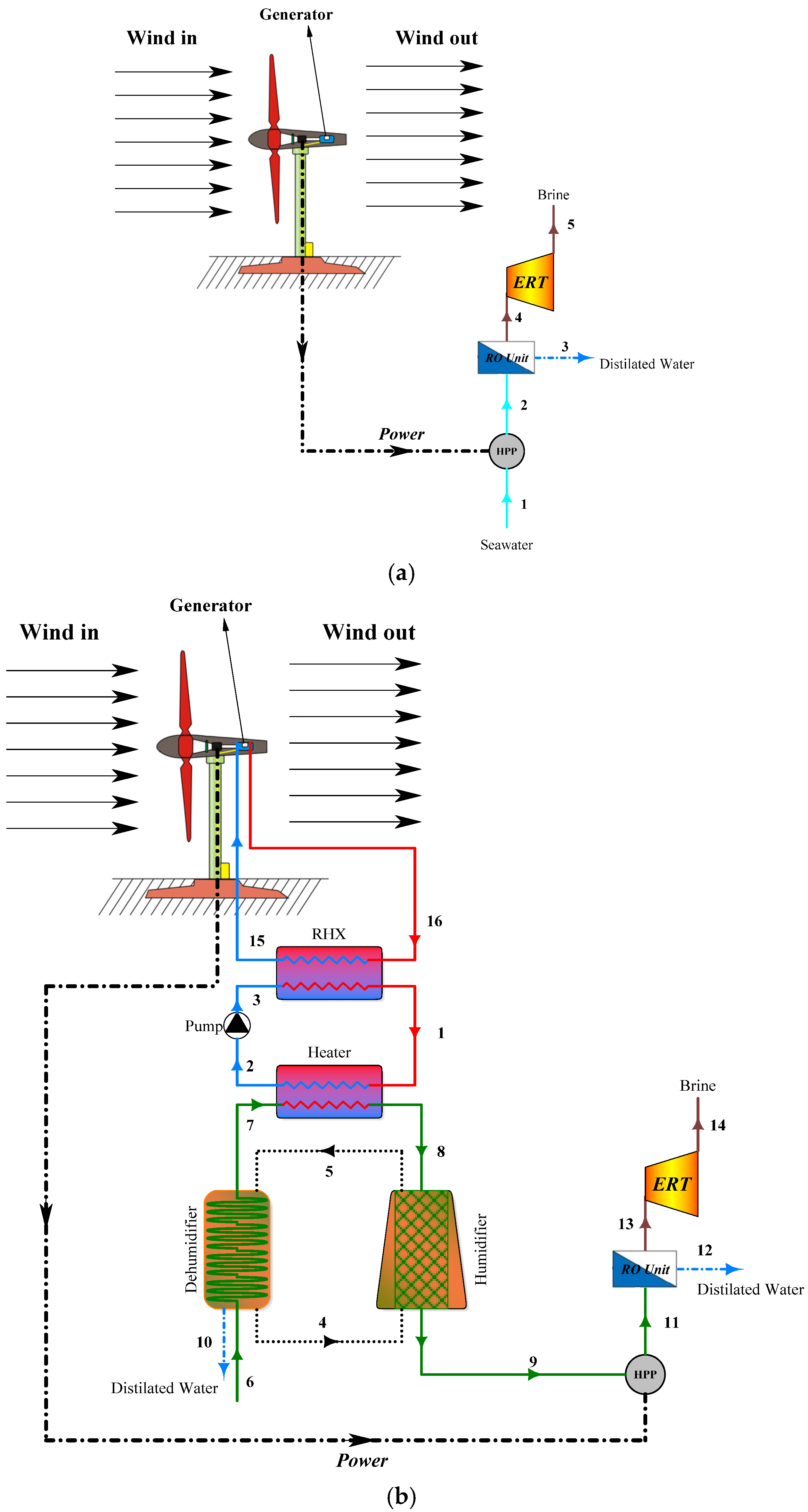
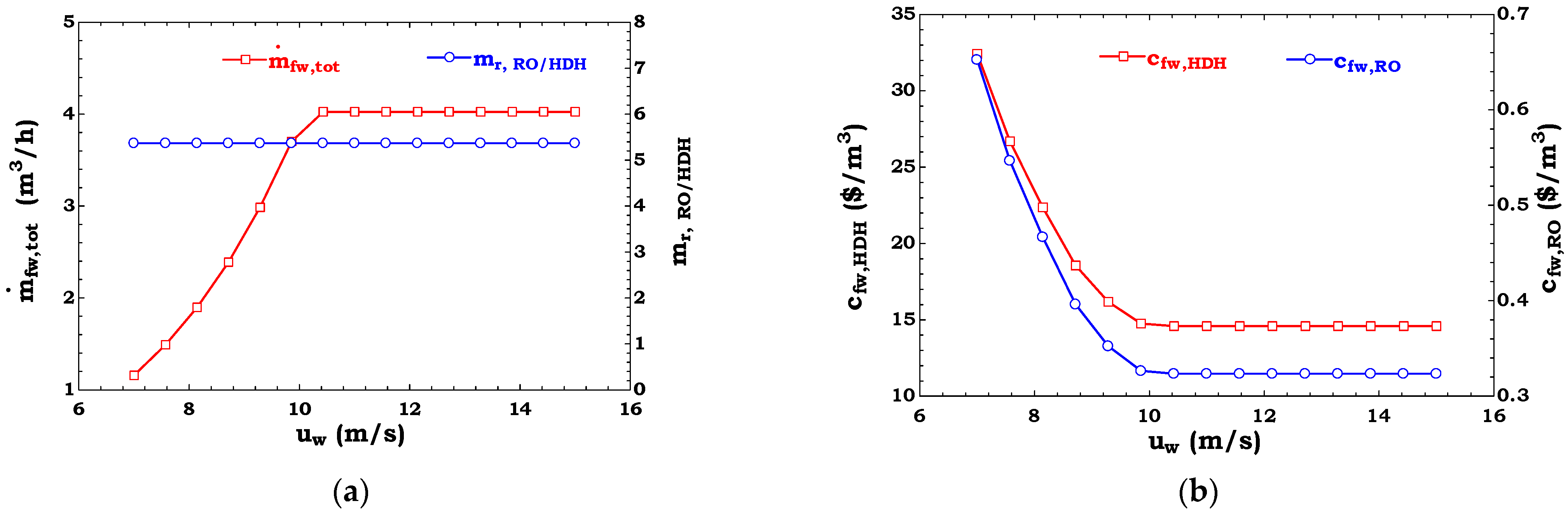
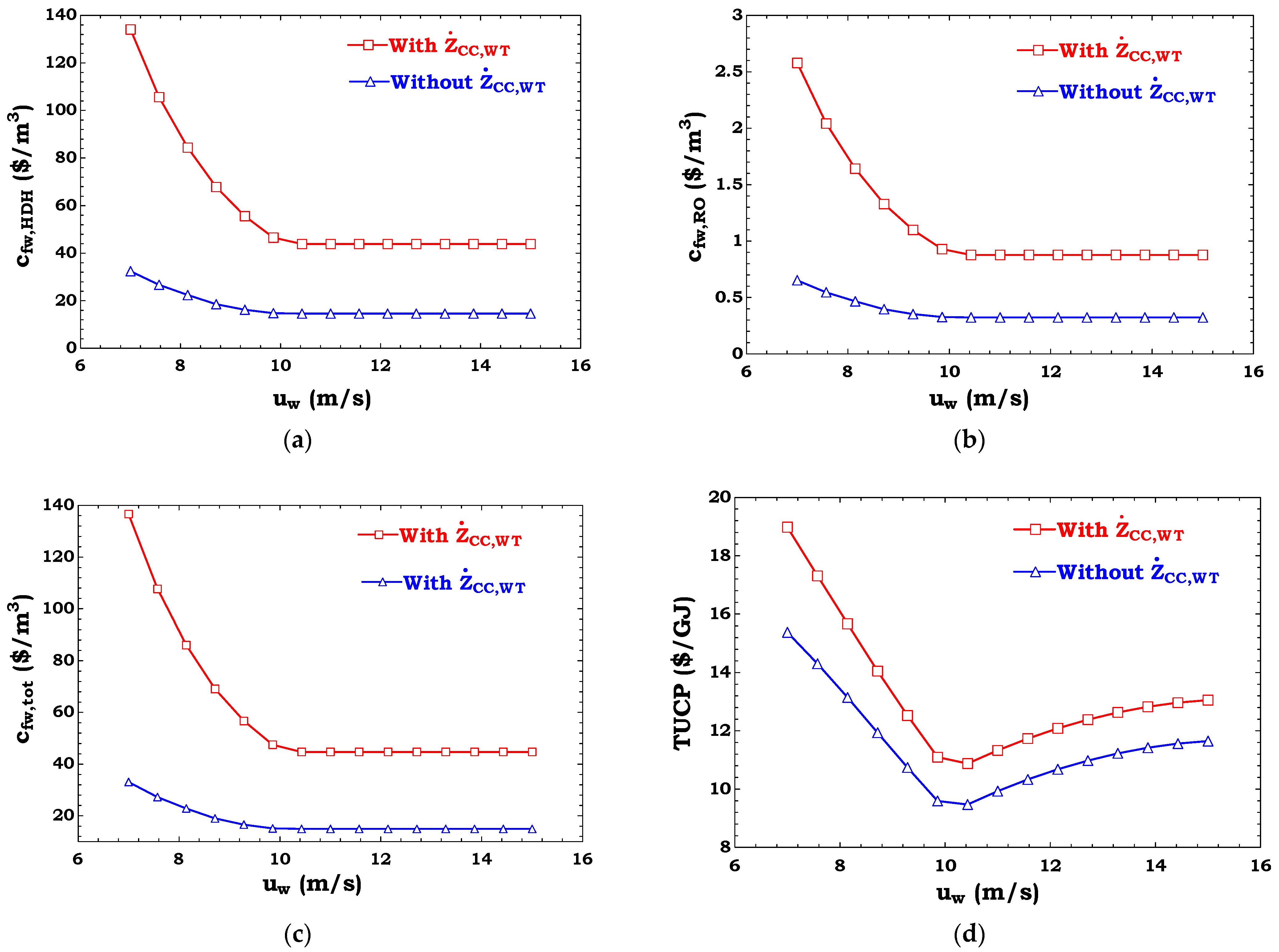
Figure 4 displays the altering trend of total freshwater rate, RO-to-HDH distilled water ratio, the unit cost of freshwater produced by the HDH sub-unit and RO sub-unit, APR, net power, SWP of the system, SWC of the hybrid unit, total exergy efficiency, the unit cost of total freshwater, TUCP, and total exergoeconomic factor with wind speed. According to Figure 4, although more freshwater is produced as the wind speed rises (since more power is supplied to the RO unit and more heat, dissipating from the generator of the wind turbine, is captured by the HDH unit), the ratio of the freshwater produced by the HDH system to that produced by the RO unit remains unchanged. This is simply because of the linear proportionality assumption made between the power and the waste heat in the applied model. In addition, the wind turbine operates at a constant maximal speed (and hence the same capacity) at wind speeds higher than the rated speed, and hence, freshwater capacity does not rise thereafter. Thus, the maximum freshwater capacity that can be obtained during the operation of the GW-136/4.5 is 4.025 m³/h. It is accepted that the unit cost associated with freshwater produced by the HDH and RO units decreases with the rise of the wind speed, since the capacity of the operating wind turbine increases, and hence it is more economical to use mechanical or thermal energies produced by the wind turbine for freshwater production at large capacities. However, the most critical point is the quantitative distribution of the unit cost between the distilled water produced by the direct supply of mechanical energy from the wind turbine and the waste heat dissipating from the generator of the wind turbine. 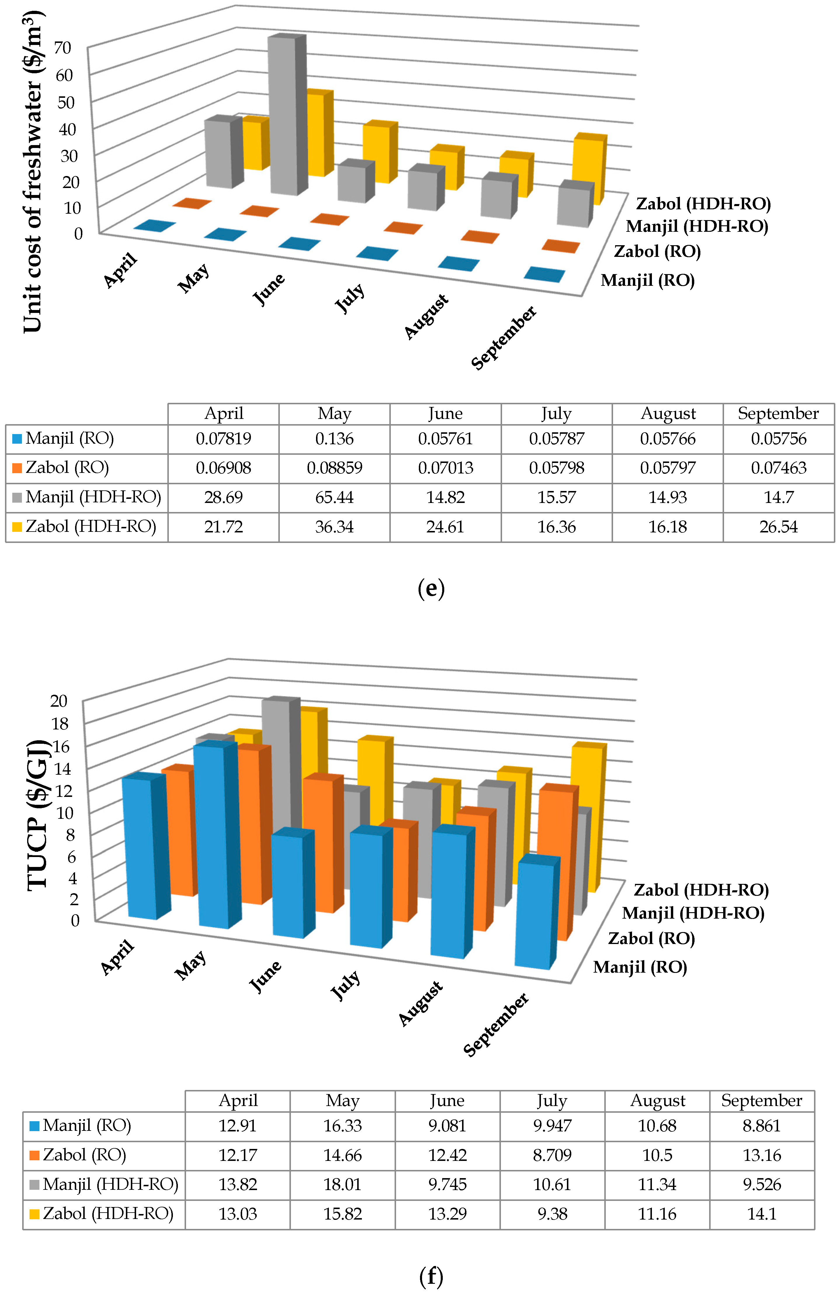According to Figure 4b, the cost of the freshwater produced by the HDH unit is inordinately higher than that produced by the RO unit. As a result, although the total freshwater rate produced through the operation of the HDH-RO unit is higher than that produced by installing a solo RO unit (as discussed in Table 7), the freshwater produced by capturing the waste heat of the generator of the wind turbine is substantially more expensive than when the power of the wind turbine is directly supplied to a mechanical desalination unit (here, an RO unit). Hence, although the idea of seawater desalination via capturing waste thermal energy of the generator of the wind turbine sounds interesting, and is explored in previous studies [5,8], no comparison is made between the unit cost of freshwater produced by each method, and the previous conclusions achieved through the analysis were incomplete. It should be noted that this conclusion is achieved with the use of a liquid-liquid cooling unit employed on the generator, and any other consideration in terms of the cooling technique might result in a less inordinate cost difference. The high unit cost of freshwater produced by the HDH unit is mainly due to the high unit cost of the steam produced after cooling down the generator, although here it is assumed that the wind turbine setup has previously been established, and the bottoming components are added on (i.e., no capital cost is considered in the cost balance equation of the wind turbine and generator, and as a result, the obtained unit cost for the steam is vastly lower when the full investment cost is accounted for).

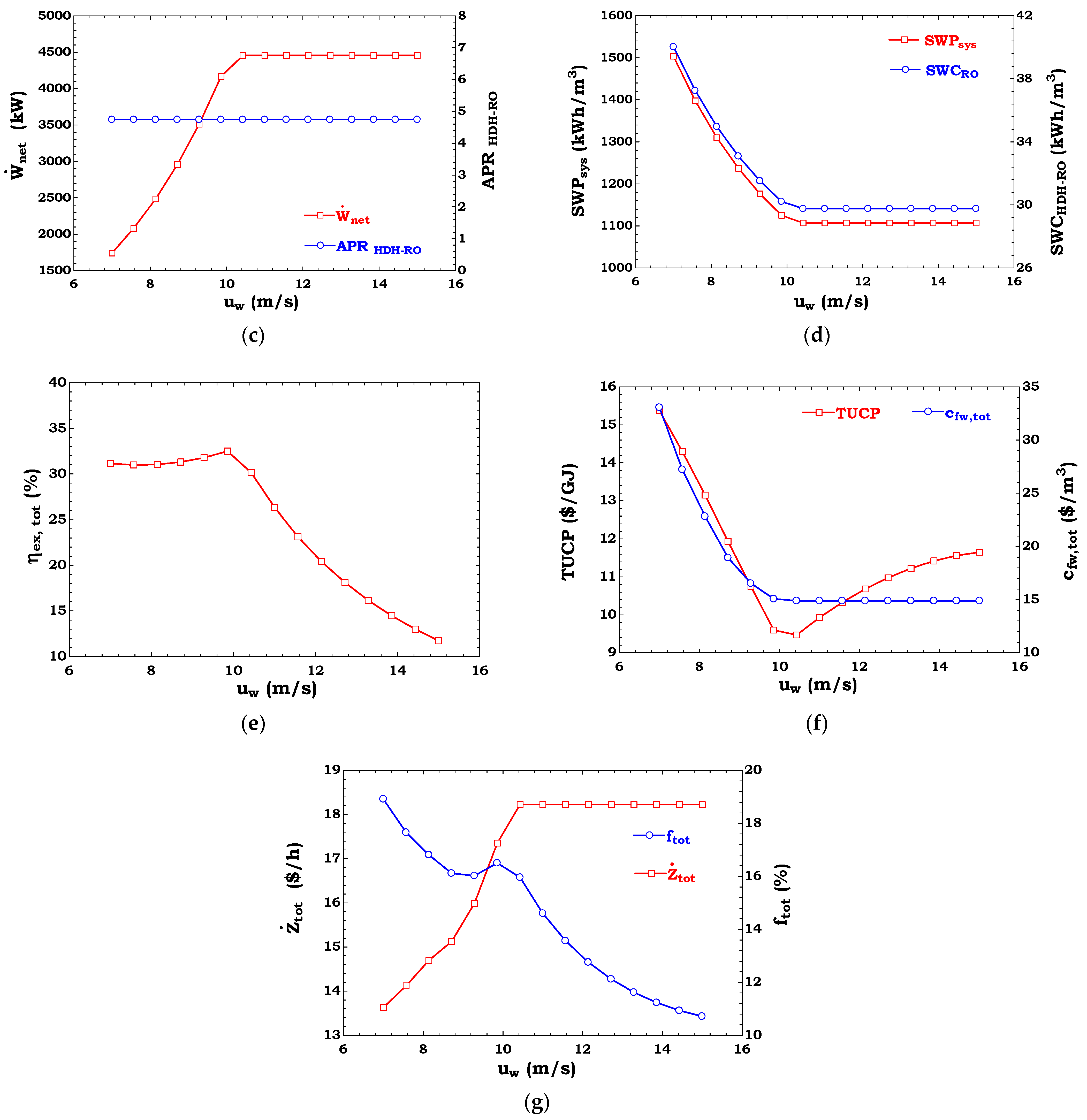
The results expressed in Figure 4 also reveal that the total exergy efficiency has reached a peak at a specific wind speed value. Quantitatively speaking, the total exergy efficiency has reached its maximum value of 32.49% at u_w = 9.85 m/s. The results of varying the exergy efficiency with the wind speed also show that the setup reveals high second-law performance at low wind speeds despite the fact that the freshwater capacity and its cost have deteriorated at this condition. That is, there is a conflicting trend between the first- and second-law metrics, or between the second-law and cost metrics, versus any change in the wind speed.

As seen earlier, the unit cost of the freshwater obtained by delivering the thermal energy of the generator of the wind turbine to the HDH unit was substantially higher than that produced by the direct supply of power to the RO unit. By accounting for the cost associated with the generated power along with the freshwater cost, one can define a single cost metric for the whole set-up, which is TUCP, as defined by Equation (66). According to the altering trend of TUCP with the wind speed, it can be stated that the TUCP can reach its minimum value of 9.47 $/GJ at a wind speed of 10.43 m/s. The wind speed at which the TUCP reaches minimum is the beginning of the point where the total freshwater cost is less affected by the wind speed (as two plots in Figure 4f show), and hence the rise in the net power cost shows its dominant effect hereafter on the TUCP.

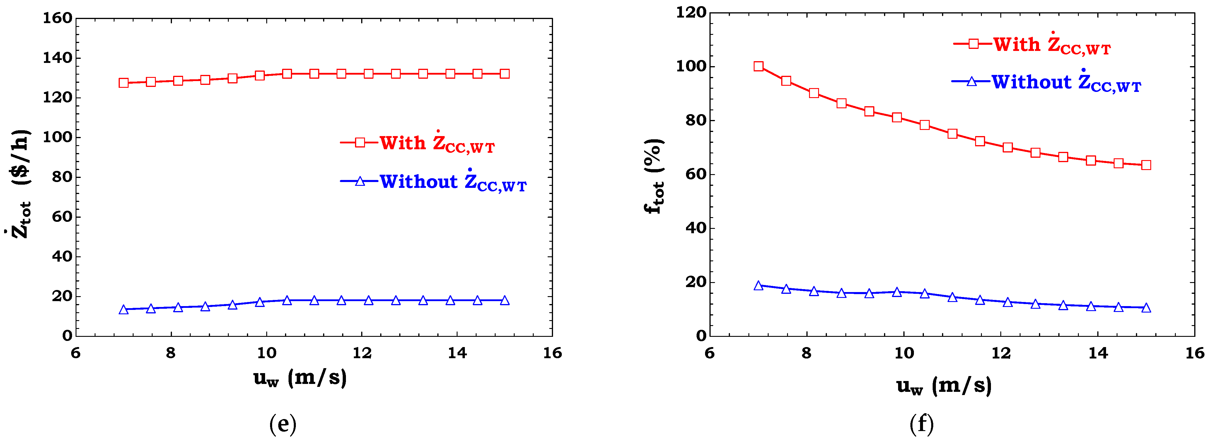
A complete cost analysis of an energy system should reveal the products’ operating cost, along with the investment cost and the cost penalty associated with the destruction, and losses occurring within the system. The varying trend of operating costs of the proposed system with wind speed was studied by introducing TUCP, or total freshwater cost. However, to have a thorough cost evaluation we have presented a variation trend of the investment cost rate and the exergoeconomic factor with the wind speed. We should reiterate that the initial capital cost of the wind turbine is not included in the total investment cost (as we have assumed that the wind turbine is previously installed). A high investment cost at high wind speed values is evident, since the scale of the required components (such as heat or mass exchangers) increases, but it remains constant for the wind speeds higher than the rated value since the capacity is unchanged. Furthermore, the significant impact of the investment cost relative to the cost rate associated with exergy destruction and loss decreases as the wind speed rises. However, it should be stated that even at low wind speeds, the value of the exergoeconomic factor is still below 50%, and hence lowering the total cost of the plant via managing the cost penalty associated with exergy destruction and loss of the system is still the top priority.

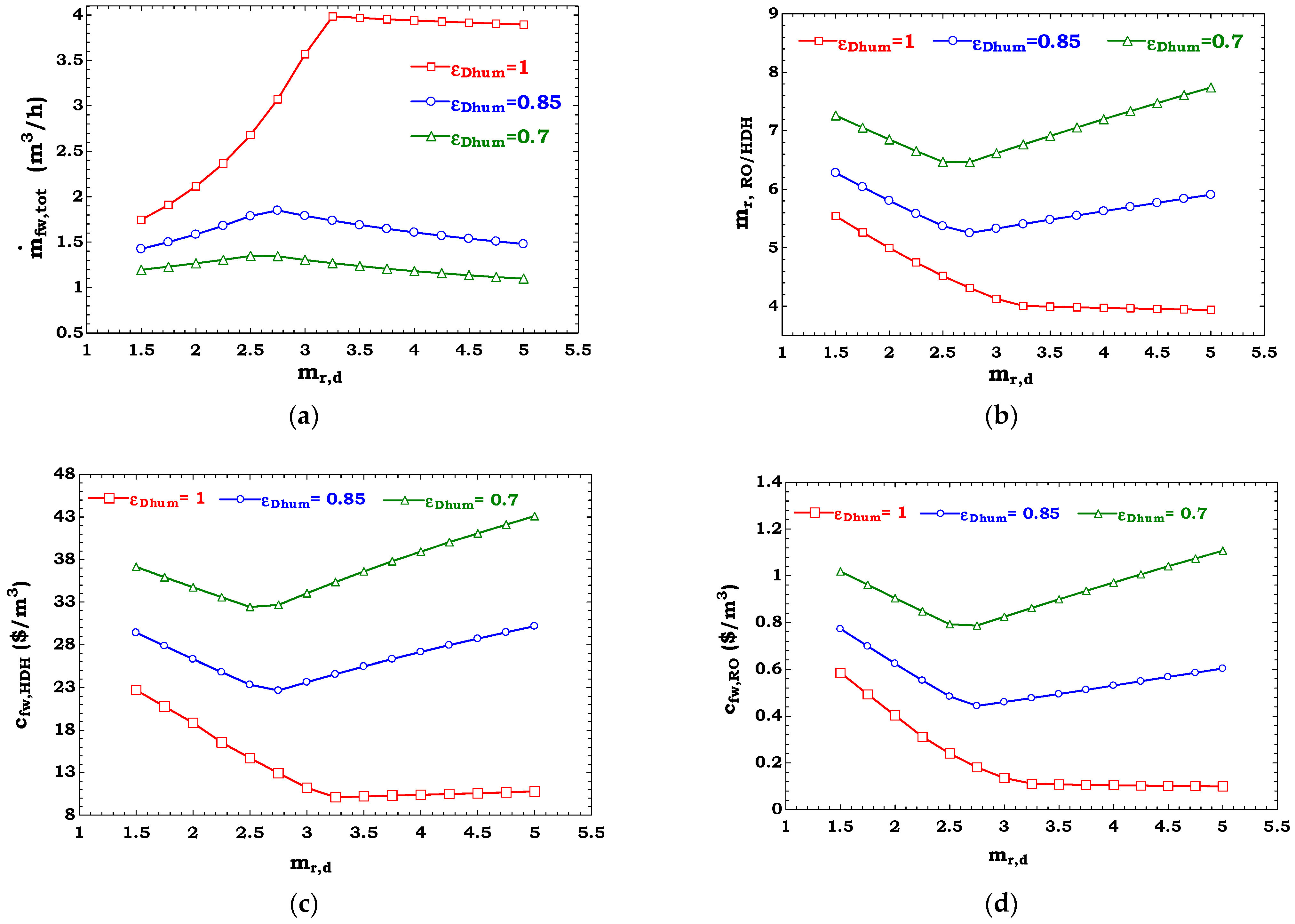
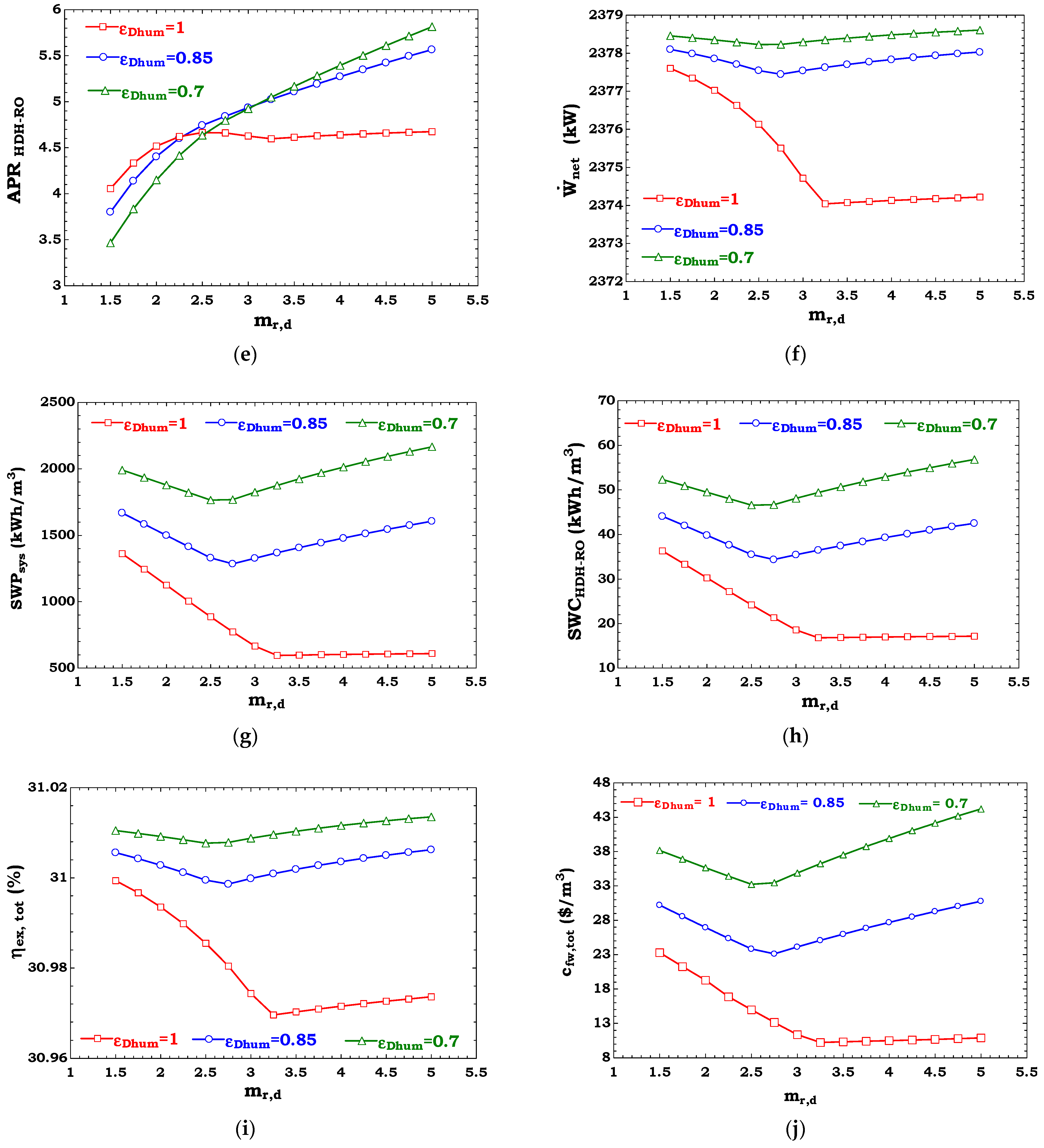
Figure 5 displays the altering trend of the total freshwater rate, RO-to-HDH distilled water ratio, unit cost of freshwater produced by the HDH sub-unit and RO sub-unit, APR, net power, SWP, SWC of the hybrid desalination unit, exergy efficiency, the unit cost of total freshwater, TUCP, and total exergoeconomic factor, with a desalination flow ratio at three different dehumidifier efficiencies of 0.7, 0.85, and 1. According to Figure 5, for each dehumidifier effectiveness level, the total freshwater rate has reached its peak value at different desalination flow ratios. In addition, as reported in previous similar studies that have investigated the effects of the dehumidifier effectiveness and desalination flow ratio on the freshwater capacity [8,31,32], this maximal freshwater capacity occurs at a higher desalination flow ratio as the dehumidifier effectiveness increases. Once the freshwater capacity increases with the rise of the desalination flow ratio at ${\epsilon }_{Dhum}=1$ up to the peak, the freshwater rate also slightly decreases thereafter, indicating the fact that setting the desalination flow ratio beyond the optimal value is advisable, since it provides rather a conservative result and the desalination capacity is less affected by any unintentional maladjustment of the optimal point in the real operation scenario. Furthermore, the results portrayed in Figure 5a indicate that increasing the dehumidifier effectiveness (with the same increment step) from 0.85 to 1 is more effective than when it is increased from 0.7 to 0.85, especially when $m_{r,d}>2$.

The contribution of each desalination sub-unit to the total freshwater capacity at different quantitative values of the desalination flow ratio, and three dehumidifier effectivenesses of 0.7, 0.85, and 1, is expressed in Figure 5b. As Figure 5b reveals, the contribution of the freshwater produced by the RO module relative to that produced by the HDH unit has its lowest amount around the optimal desalination flow ratio (where the total freshwater rate is maximal). It should be emphasized that the freshwater produced by each unit has a maximum point relative to the desalination flow ratio near the same optimal desalination flow ratio. However, the freshwater produced by the HDH unit hugely affects the RO-to-HDH flow ratio, due to its high varying rate.

To understand how the unit cost of the freshwater produced by each desalination unit is affected through varying the desalination flow ratio and the dehumidifier effectiveness, please see Figure 5c,d. First and foremost, a comparison between the unit cost of the freshwater produced via each unit substantiates the previous concluding remark about the high cost of the freshwater of the HDH unit compared to the RO unit. The aggregated unit cost of the freshwater (Figure 5k) shows a similar trend of change to each individual unit cost, due to the same varying behavior of both parameters, and its quantitative value is very similar to that of the HDH unit, due to its dominant cost.

With the rise of the desalination flow ratio, the humidity of the humidified air leaving the humidifier increases, while the dry air mass flow rate decreases substantially. By considering the rise in the freshwater rate at low desalination flow ratios and the drop in the freshwater rate at high desalination flow ratios, via increasing the desalination flow ratio along with the decrease in the dry air flow rate, through this change, it can be declared that the APR of the hybrid HDH-RO unit increases considerably and continuously at low dehumidifier effectiveness, and its increment rate decreases at higher dehumidifier effectiveness. That is, at ${\epsilon }_{Dhum}=1$ the APR increases with the rise of the desalination flow ratio at lower desalination flow ratio values, while it slightly decreases and remains nearly constant thereafter.

Three additional significant metrics, including of the net power, SWC of the hybrid HDH-RO desalination unit, and SWP of the whole setup, are also included here, and their varying trend with the change of the desalination flow ratio and dehumidifier effectiveness is plotted in Figure 5f–h, respectively. On this basis, since the power produced by the wind turbine is constant and independent of any change in the desalination flow ratio and dehumidifier effectiveness, only the power recovered by the ERT is changing. Accordingly, the power produced by the ERT has a maximum value with the change of the desalination flow ratio and increases as the dehumidifier effectiveness increases. As a result, it affects the net power inversely, and hence the net power will have a minimum point versus a broad change of the desalination flow ratio, where the severity of the drop in the net power at lower desalination flow ratios and higher dehumidifier effectiveness is relatively high, although the scale of the power recovered by the ERT is meaningfully smaller than the power generated by the wind turbine. Due to the direct relationship of the SWP to the net power and inverse relationship with the total freshwater rate, the SWP of the system will be affected in the same direction from both of these influential parameters, and hence its altering trend versus the desalination flow ratio and dehumidifier effectiveness will resemble that of the net power. The same altering trend is predictable for the SWC of the hybrid HDH-RO desalination system, since it is inversely affected by the total freshwater rate and the ERT power.

According to the altering trend of TUCP with the desalination flow ratio at different values of dehumidifier effectiveness, it can be stated that the TUCP can reach its maximum value at ${\epsilon }_{Dhum}=0.7 \mathrm{and} 0.85$, while increasing at two different increment rates at ${\epsilon }_{Dhum}=1$. Therefore, by operating the HDH unit with a low desalination flow ratio, one can considerably lower the TUCP, although lowering the dehumidifier effectiveness to pursue lowering the TUCP is effective as well. However, there is a conflicting trend of interest in the TUCP, and the unit cost associated with total freshwater, in terms of selecting the ultimate values of dehumidifier effectiveness or the desalination flow ratio that must be taken into account prior to the final decision. Since the altering trend of the unit cost of the total freshwater rate is hugely affected by the desalination flow ratio as well as the dehumidifier effectiveness, its varying trend can be prioritized over the TUCP in the ultimate design stage. The exergoeconomic factor, defined as the ratio of the investment cost rate to the cost rate associated with exergy destruction and loss, as well as the investment cost rate, has reached a peak value as its varying tendency with the desalination flow ratio is investigated. It should be stated that through the range of the investigated parameters, the value of the exergoeconomic factor is still below 50%, and hence, lowering the total cost of the plant via lowering the cost penalty associated with the destruction and losses of the exergy of the system is still the top priority. Since the operating and maintenance cost of the wind turbine (as the topping system) remains unchanged with the change of the desalination flow ratio or the dehumidifier effectiveness, the exergoeconomic factor changes slightly through this alteration and cannot be lowered significantly with each of these two design parameters.

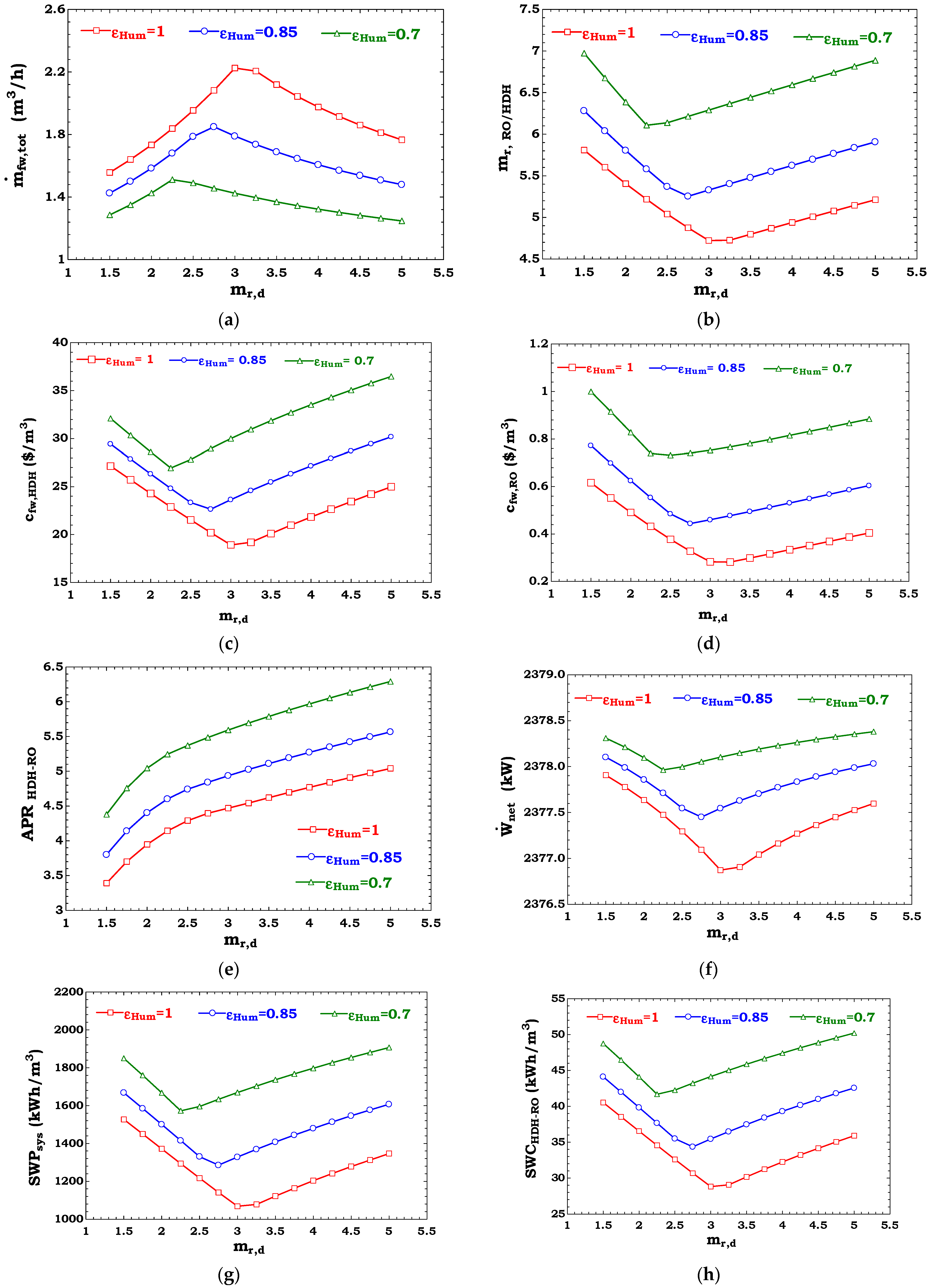
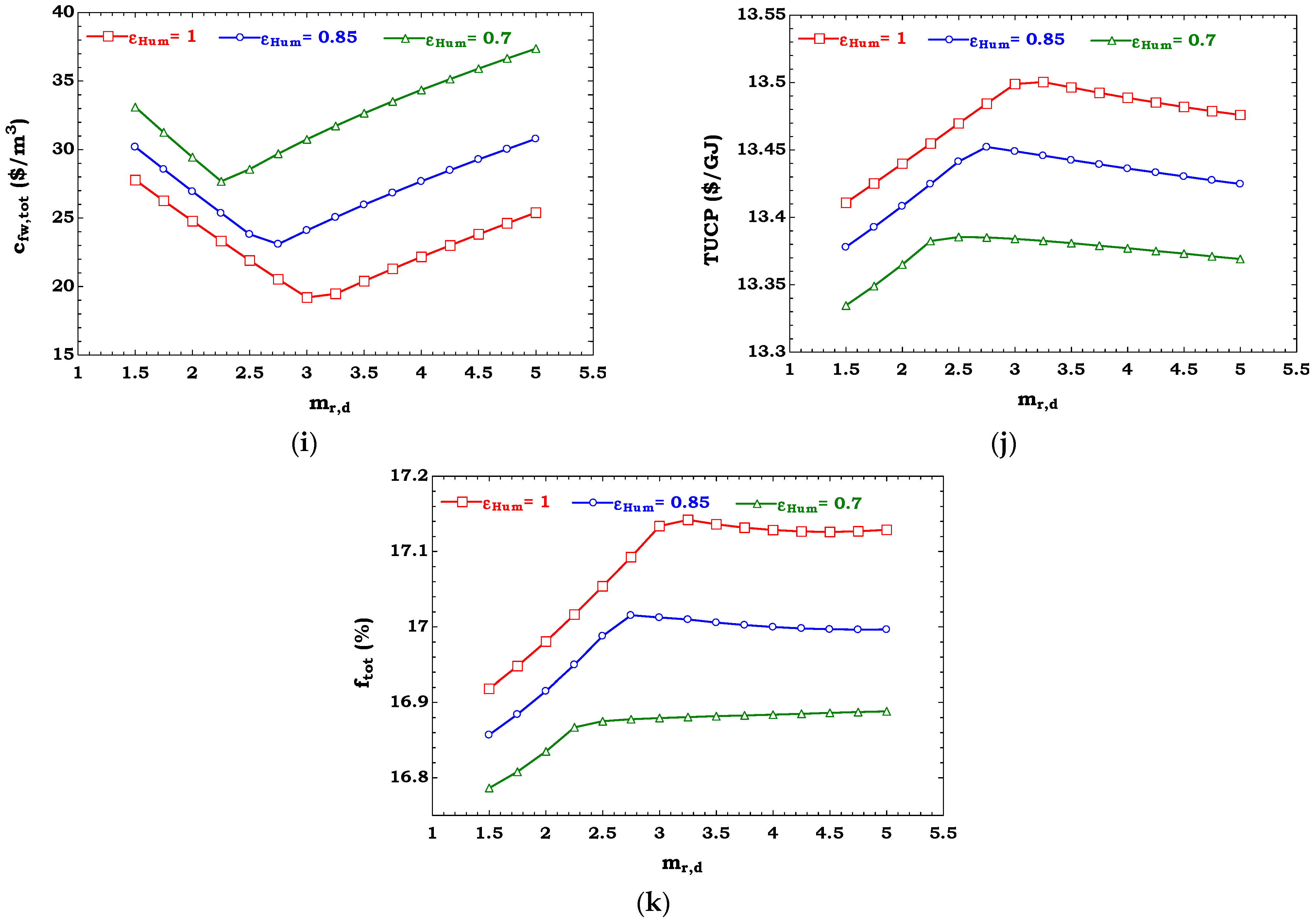
Figure 6 displays the altering trend of the total freshwater rate, RO-to-HDH distilled water ratio, unit cost of freshwater produced by the HDH sub-unit and RO sub-unit, APR, net power, SWP, SWC of the hybrid unit, the unit cost of total freshwater, TUCP, and total exergoeconomic factor, with a desalination flow ratio at three different humidifier effectiveness levels of 0.7, 0.85, and 1. The variation trend of the exergy efficiency is excluded here, due to its very slight change.

According to Figure 6, for each humidifier effectiveness, the total freshwater rate has reached its peak value at different desalination flow ratios. As also reported in previous similar studies investigating the influence of humidifier effectiveness and desalination flow ratio on the freshwater capacity [8,31,32], this maximal freshwater capacity occurs at higher desalination flow ratios as the humidifier effectiveness increases. In addition, as has been demonstrated in these studies [8,31,32], once we compare the results of Figure 5a and Figure 6a, it can be stated that the influence of the dehumidifier effectiveness on the freshwater capacity is more meaningful than that of the humidifier effectiveness. The altering trend of all metrics versus the humidifier effectiveness is the same as the dehumidifier effectiveness, for nearly the same reasons which were explained previously, except for the following differences. In contrast to the observation that the freshwater capacity slightly decreased with the rise of the desalination flow ratio at ${\epsilon }_{Dhum}=1$ from the maximal point thereafter, here it has dropped significantly, like the varying trend observed at lower humidifier effectiveness levels. Furthermore, despite the different increment/decrement rate seen in Figure 5a for different values of dehumidifier effectiveness, Figure 6a shows that increasing the humidifier effectiveness (with the same increment step) from 0.85 to 1 has the same effect when it is increased from 0.7 to 0.85. Hence, the altering shape of the total freshwater rate with desalination flow ratio is independent of the humidifier effectiveness. In addition, in contrast to the results captured in Figure 5e, Figure 6e indicates that the variation of the APR with the desalination flow ratio at all humidifier effectiveness levels is similar, with nearly the same varying slope but with an up- or downward shift relative to each other. Hence, the altering shape of the APR with the desalination flow ratio is independent of the humidifier effectiveness. In addition, as Figure 5k indicated, the TUCP reached its maximum value at ${\epsilon }_{Dhum}=0.7 \mathrm{and} 0.85$, while it increased by two different increment rates at ${\epsilon }_{Dhum}=1$. However, here the alteration pattern of the TUCP with the desalination flow ratio is the same for all three investigated humidifier effectiveness levels.

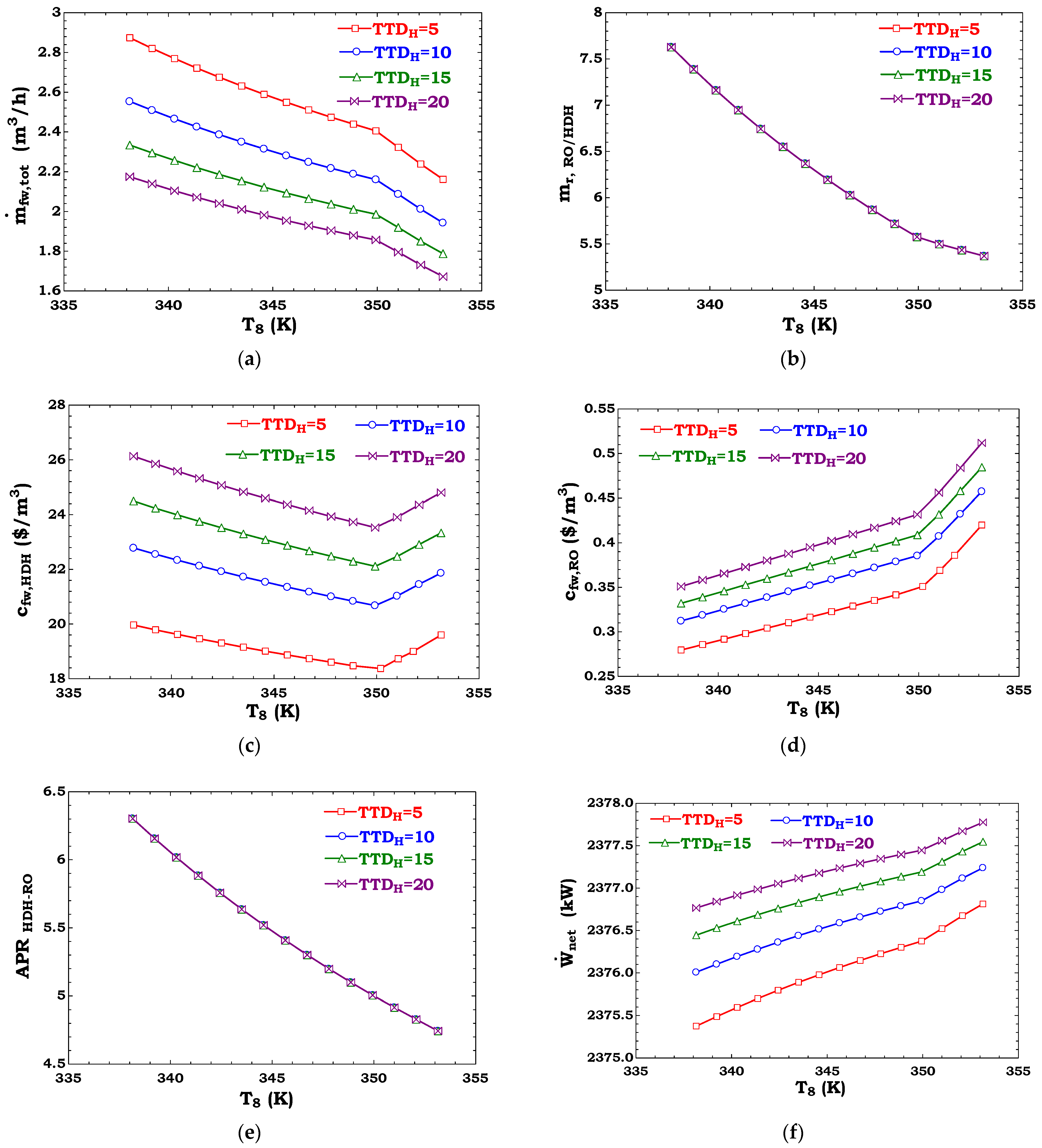
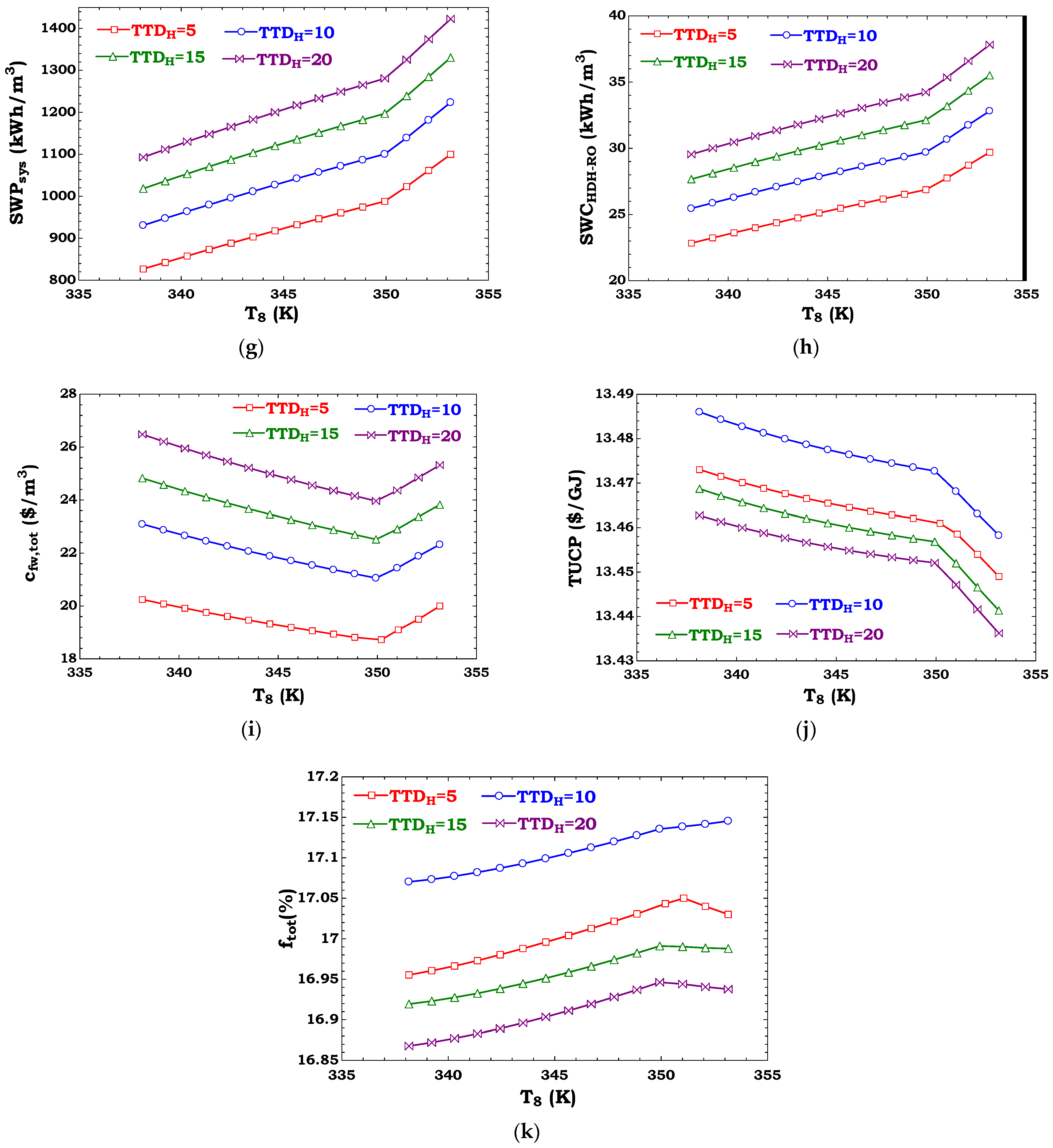
Figure 7 displays the altering trend of the total freshwater rate, RO-to-HDH distilled water ratio, unit cost of freshwater produced by the HDH sub-unit and RO sub-unit, APR, net power, SWP, SWC of the hybrid unit, unit cost of total freshwater, TUCP, and total exergoeconomic factor with desalination top temperature at four different TTDs of the heater at 5, 10, 15, and 20 K. The altering trend of the total exergy efficiency is excluded here, due to its constant trend with the TTD of the heater and the desalination top temperature. According to Figure 7, the total freshwater rate increases with the drop of the desalination top temperature or TTD of the heater. It should be noted that at low values of the TTD of the heater, the amount of fresh water can be enhanced more significantly than is the case when the system works at higher TTDs of the heater. That is, when decreasing the TTD of the heater with a constant decrement step of 5 K, decreasing from 10 K to 5 K is more effective than when it is decreased from 20 K to 15 K, especially at lower desalination top temperatures.

The contribution of each desalination sub-unit to total freshwater capacity at different quantitative values of the desalination top temperature and four TTDs of the heater of 5 K, 10 K, 15 K, and 20 K is expressed in Figure 7b. As Figure 7b reveals, varying the TTD of the heater makes no contribution to the proportion of the freshwater produced by the RO module, relative to that produced by the HDH unit. The RO-to-HDH freshwater ratio only decreases with the rise of the desalination top temperature, since the contribution of the HDH unit at a high scale of the operating temperature will obviously increase its role in the total freshwater rate.

To understand how the unit cost of the freshwater produced by each desalination unit is affected through varying the desalination top temperature and the TTD of the heater, please see Figure 7c,d. First and foremost, a comparison between the unit cost of the freshwater produced via each unit substantiates the previously made concluding remark about the high cost of the freshwater of the HDH unit compared to the RO unit. In addition, by setting the operating desalination top temperature at higher values, one can expect to lower the high unit cost of freshwater of the HDH unit relative to that of the RO unit, although it is still high and is not economical. The aggregated unit cost of the freshwater (Figure 7i) shows a similar trend of change to the unit cost of the freshwater of the HDH unit, due to the dominant role of this element.

With the rise of the desalination top temperature, the humidity of the air leaving the humidifier increases, while the dry air mass flow rate decreases substantially. By considering the drop in the freshwater rate and the dry air mass flow with the rise of the desalination top temperature, it can be stated that the APR of the hybrid HDH-RO unit will decrease continuously. Regarding the altering trend of the net power, since the power produced by the wind turbine is constant with the change of the desalination top temperature and the TTD of the heater, only the power produced by the ERT meaningfully decreases (although the power consumed by the pump is decreasing as well) with the rise of the desalination top temperature or TTD of the heater. Therefore, the net power will increase with the rise of the desalination top temperature or TTD of the heater. It should be noted that at low values of TTD of the heater the amount of the net power can be enhanced more significantly than the case when the system works at a higher TTD of the heater. That is, increasing the TTD of the heater with a constant increment step of 5 K from 5 K to 10 K is more effective than when it is increased from 15 K to 20 K.

Due to the direct relationship of the SWP with the net power, and its inverse relationship with the total freshwater rate, the SWP of the system will be affected in the same direction from both of these influential parameters, and hence, its altering trend versus those of the desalination top temperature and TTD of the heater will resemble that of the net power. The same altering trend is predictable for the SWC of the hybrid HDH-RO desalination system, since it is inversely affected by the total freshwater rate and the ERT power, and hence, both SWP and SWC will increase with the rise of the desalination top temperature and TTD of the heater.

According to the altering trend of TUCP with the desalination top temperature at different values of the TTD of the heater, it can be stated that the TUCP decreases with the rise of the desalination top temperature. Meanwhile, the TUCP first increases as the TTD of the heater increases from 5 K to 10 K, and hence decreases as the TTD of the heater increases from 10 K to 20 K. Therefore, there is a conflicting trend of interest in the TUCP and the unit cost associated with total freshwater in terms of selecting the ultimate values of the TTD of the heater, which must be taken into account prior to the final decision. Since the altering trend of the unit cost of the total freshwater rate is hugely affected by the TTD of the heater, its varying trend can be prioritized over the TUCP in the ultimate design stage. The exergoeconomic factor increases with the rise of the desalination top temperature, while it is increased as the TTD of the heater increases from 5 K to 10 K, and hence is decreased as the TTD of the heater increases from 10 K to 20 K. It should be stated that through the range of these two investigated parameters (i.e., $T_8$ and $TT{D}_H$), the value of the exergoeconomic factor is still below 50%, and hence, lowering the cost penalty associated with the destruction and losses of the exergy of the system is still the top priority.

5.3. Waste Heat Recovery from an Installed or a New Wind Turbine

As mentioned earlier, the economic modeling of the devised hybrid HDH-RO desalination system driven by the waste heat and electrical power of the wind turbine was carried out under the key assumption that the wind turbine setup exists previously, and hence, only the operating and maintenance cost of the wind turbine is accounted for in the cost balance equations of the wind turbine and its generator. This assumption is drawn mainly because of the fact that waste heat recovery from the generator of the wind turbine is practically feasible only when the wind turbine has been installed previously, and hence its capital cost rate does not affect the unit cost of the steam produced by the generator. Once the capital cost rate is also included in the cost balance equations of the wind turbine and its generator, it is seen that the unit cost of this steam is irrationally surged and leads to astronomical cost metrics. This part is set to calculate the ultimate cost metrics of the hybrid WT/HDH-RO system at various wind speeds, when the capital cost is included in the cost balance equations.

According to Figure 8, it can be stated that all cost metrics of the system with the inclusion of the capital cost of the wind turbine and its generator are higher than when only the operating and maintenance cost of the wind turbine setup was considered, as expected before. More specifically, for wind speeds lower than around 10 m/s, the unit cost of the freshwater produced by the HDH unit, RO unit, and the summation of these two streams is significantly high for the case when the capital cost of the wind turbine and its generator is included, which makes theoretical results less rational. Therefore, in spite of previous cost modeling [5,6,8,9] which has accounted for capital cost in the exergoeconomic balance equations, it seems that such deliberation leads to inaccurate cost assessment from the wind turbine waste heat recovery concept.

5.4. Case Study

Figure 9 portrays the monthly averaged meteorology data for a representative day for both cities of Manjil and Zabol. Based upon the extracted data in the presented form, the results of the simulation are extended through this representative day, and the results are portrayed in Figure 10. It should be noted that the wind turbine virtually shuts down at velocities below the cut-in speed and does not achieve speeds higher than the rated speed.

Figure 10 presents the monthly total freshwater rate, net power, SWC of the hybrid HDH-RO unit, exergy efficiency, unit cost of the total freshwater rate, and TUCP values for the two locations of Manjil and Zabol. According to Figure 10a,b, in Manjil, more freshwater and power are produced from June to September, while in Zabol, the rate of freshwater and net power in July and August are high. In all investigated scenarios, the rate of freshwater produced by the HDH-RO unit is higher than that produced by the reference system.

The amount of net electricity produced in June to September (in Manjil) and July and August (in Zabol) is the same because in some cases the average wind speed (at z = 86 m) is higher than the rated wind speed of the wind turbine, and hence the wind turbine works at a constant capacity. As a result, the SWC value in June to September (in Manjil) and July and August (in Zabol) is at the lowest value (Figure 10c). The results of the second-law analysis reveal that, for the Zabol city, the exergy efficiency of the HDH-RO and solo RO units in June and July is considerably high, while, for the Manjil city, the highest amount of the exergy efficiency for both HDH-RO and solo RO units occurs in September.

Figure 10e,f reveals quantitative values for the unit cost of freshwater and TUCP for both hybrid and reference systems. Accordingly, the lowest TUCP and unit cost of freshwater for Manjil occurred in September, while the highest value occurred in May. For Zabol, the lowest TUCP and unit cost of freshwater occurred in July, while the highest value occurred in May.

6. Conclusions

In this study, an HDH unit was used to capture the waste heat of the generators of various wind turbine models for seawater desalination. Cu/water was used in the liquid-liquid cooling system of the wind turbine, and the waste brine stream exiting from the HDH unit was fed into a RO unit for more freshwater production. The superiorities and inferiorities of the devised layout versus the RO unit were comprehensively discussed in terms of thermodynamics and thermoeconomics. The study explicitly criticized the economic aspect of waste heat recovery from the generator of the wind turbine for seawater desalination via HDH, versus the RO unit, due to the following reasons: (i) it was found that more power can be recovered from the discarded brine from the solo RO unit than the hybrid HDH-RO unit, (ii) the solo RO desalination system, working directly with the power of the wind turbine, has a less complex configuration, and hence its investment cost rate was remarkably lower than that needed for setting an HDH-RO unit, and (iii) the unit cost associated with the freshwater produced by the HDH unit was astronomical when it was compared with that of the RO unit.

Among all screened wind turbines, the GW-136/4.8 was recommended, due to greater power generation, but its investment cost rate was high. However, the freshwater unit cost of the GW-136/4.8 was significantly lower than the values obtained for other models. The maximum freshwater capacity during the operation of the GW-136/4.5 was 4.025 m³/h. The total exergy efficiency had reached its maximum value of 32.49% at u_w = 9.85 m/s, while the TUCP reached its minimum value of 9.47 $/GJ at a wind speed of 10.43 m/s. The results of varying the exergy efficiency with the wind speed also demonstrated that the set-up reveals a high second-law performance at low wind speeds, despite the fact that the freshwater capacity and its cost deteriorated under these conditions. In all investigated conditions, the value of the exergoeconomic factor was below 50%, and hence, lowering the total cost of the plant via managing the cost penalty associated with exergy destruction and the loss of the system is the top priority.

In addition, there is a conflicting trend of interest in the TUCP and the unit cost associated with total freshwater, in terms of selecting the ultimate values of dehumidifier effectiveness or the desalination flow ratio, which must be taken into account prior to the final decision. The TUCP reached its maximum value at ${\epsilon }_{Dhum}=0.7 \mathrm{and} 0.85$, while it increased with two different increment rates at ${\epsilon }_{Dhum}=1$. However, when varying the humidifier effectiveness, the alteration pattern of the TUCP with the desalination flow ratio is the same for all three investigated humidifier effectiveness levels, and it demonstrates a peak point.

At low values of the TTD of the heater, the amount of fresh water can be enhanced more significantly than is the case when the system works at the higher TTDs of the heater. There was a conflicting trend of interest in the TUCP and the unit cost associated with total freshwater, in terms of selecting the ultimate values of the TTD of the heater, which must be taken into account prior to the final decision. Since the altering trend of the unit cost of the total freshwater rate is hugely affected by the TTD of the heater, its varying trend can be prioritized over the TUCP in the final design stage.

References

1. Kudelin, A.; Kutcherov, V. Wind ENERGY in Russia: The current state and development trends. Energy Strategy Rev. 2021, 34, 100627. [Google Scholar] [CrossRef]
2. Tong, W. Wind Power Generation and Wind Turbine Design; WIT Press: San Francisco, CA, USA, 2010. [Google Scholar]
3. Yuan, W.; Jiang, Y. Cooling Systems in Wind Turbine. World Sci-Tech R D 2007, 29, 80–85. [Google Scholar]
4. Tian-jun, N. Major Cooling Methods and Features of Large Generator. Dongfang Electr. Rev. O 2006, 2, 31–37. [Google Scholar]
5. Khalilzadeh, S.; Nezhad, A.H. Utilization of waste heat of a high-capacity wind turbine in multi effect distillation desalination: Energy, exergy and thermoeconomic analysis. Desalination 2018, 439, 119–137. [Google Scholar] [CrossRef]
6. Khalilzadeh, S.; Nezhad, A.H. Using waste heat of high capacity wind turbines in a novel combined heating, cooling, and power system. J. Clean. Prod. 2020, 276, 123221. [Google Scholar] [CrossRef]
7. De Risi, A.; Milanese, M.; Colangelo, G.; Laforgia, D. High efficiency nanofluid cooling system for wind turbines. Therm. Sci. 2014, 18, 543–554. [Google Scholar]
8. Rostamzadeh, H.; Rostami, S. Performance enhancement of waste heat extraction from generator of a wind turbine for freshwater production via employing various nanofluids. Desalination 2020, 478, 114244. [Google Scholar] [CrossRef]
9. Rostami, S.; Rostamzadeh, H.; Fatehi, R. A new wind turbine driven trigeneration system applicable for humid and windy areas, working with various nanofluids. J. Clean. Prod. 2021, 296, 126579. [Google Scholar] [CrossRef]
10. Nayar, K.G.; Fernandes, J.; McGovern, R.K.; Al-Anzi, B.S. Cost and energy needs of RO-ED-crystallizer systems for zero brine discharge seawater desalination. Desalination 2019, 457, 115–132. [Google Scholar] [CrossRef]
11. Nayar, K.G.; Fernandes, J.; McGovern, R.K.; Dominguez, K.P.; McCance, A.; Al-Anzi, B.S. Cost and energy requirements of hybrid RO and ED brine concentration systems for salt production. Desalination 2019, 456, 97–120. [Google Scholar] [CrossRef]
12. Han, X.; Zhang, D.; Yan, J.; Zhao, S.; Liu, J. Process development of flue gas desulphurization wastewater treatment in coal-fired power plants towards zero liquid discharge: Energetic, economic and environmental analyses. J. Clean. Prod. 2020, 261, 121144. [Google Scholar] [CrossRef]
13. Mohamed, E.S.; Papadakis, G. Design, simulation and economic analysis of a stand-alone reverse osmosis desalination unit powered by wind turbines and photovoltaics. Desalination 2004, 164, 87–97. [Google Scholar] [CrossRef]
14. Segurado, R.; Madeira, J.; Costa, M.; Duić, N.; Carvalho, M.G. Optimization of a wind powered desalination and pumped hydro storage system. Appl. Energy 2016, 177, 487–499. [Google Scholar] [CrossRef] [Green Version]
15. Gorjian, S.; Ghobadian, B. Solar desalination: A sustainable solution to water crisis in Iran. Renew. Sustain. Energy Rev. 2015, 48, 571–584. [Google Scholar] [CrossRef]
16. Mostafaeipour, A.; Abarghooei, H. Harnessing wind energy at Manjil area located in north of Iran. Renew. Sustain. Energy Rev. 2008, 12, 1758–1766. [Google Scholar] [CrossRef]
17. Iranian Meteorological Organization (IMO). 2018. Available online: http://www.irimo.ir/eng/index.php (accessed on 30 June 2021).
18. Ashrafi Goudarzi, S.; Fazelpour, F.; Gharehpetian, G.B.; Rosen, M.A. Techno-economic assessment of hybrid renewable resources for a residential building in tehran. Environ. Prog. Sustain. Energy 2019, 38, 13209. [Google Scholar] [CrossRef]
19. Nafey, A.; Sharaf, M. Combined solar organic Rankine cycle with reverse osmosis desalination process: Energy, exergy, and cost evaluations. Renew. Energy 2010, 35, 2571–2580. [Google Scholar] [CrossRef]
20. Namin, A.S.; Rostamzadeh, H.; Nourani, P. Thermodynamic and thermoeconomic analysis of three cascade power plants coupled with RO desalination unit, driven by a salinity-gradient solar pond. Therm. Sci. Eng. Prog. 2020, 18, 100562. [Google Scholar] [CrossRef]
21. Rostamzadeh, H. Indirect mechanical heat pump assisted humidification-dehumidification desalination systems. Int. J. Energy Res. 2021. [Google Scholar] [CrossRef]
22. Bejan, A.; Tsatsaronis, G.; Moran, M.J. Thermal Design and Optimization; John Wiley & Sons: Hoboken, NJ, USA, 1995. [Google Scholar]
23. Said, Z.; Saidur, R.; Sabiha, M.; Hepbasli, A.; Rahim, N. Energy and exergy efficiency of a flat plate solar collector using pH treated Al2O3 nanofluid. J. Clean. Prod. 2016, 112, 3915–3926. [Google Scholar] [CrossRef]
24. Wepfer, W.; Gaggioli, R.; Obert, E. Proper evaluation of available energy for HVAC. ASHRAE Trans. 1979, 85, 214–230. [Google Scholar]
25. Turton, R.; Bailie, R.C.; Whiting, W.B.; Shaeiwitz, J.A. Analysis, Synthesis and Design of Chemical Processes; Pearson Education: London, UK, 2008. [Google Scholar]
26. Hall, S.; Ahmad, S.; Smith, R. Capital cost targets for heat exchanger networks comprising mixed materials of construction, pressure ratings and exchanger types. Comput. Chem. Eng. 1990, 14, 319–335. [Google Scholar] [CrossRef]
27. Kim, J.-K.; Savulescu, L.; Smith, R. Design of cooling systems for effluent temperature reduction. Chem. Eng. Sci. 2001, 56, 1811–1830. [Google Scholar] [CrossRef]
28. El-Emam, R.S.; Dincer, I. Thermodynamic and thermoeconomic analyses of seawater reverse osmosis desalination plant with energy recovery. Energy 2014, 64, 154–163. [Google Scholar] [CrossRef]
29. Rostamzadeh, H.; Ghiasirad, H.; Amidpour, M.; Amidpour, Y. Performance enhancement of a conventional multi-effect desalination (MED) system by heat pump cycles. Desalination 2020, 477, 114261. [Google Scholar] [CrossRef]
30. Narayan, G.P.; McGovern, R.K.; Zubair, S.M. High-temperature-steam-driven, varied-pressure, humidification-dehumidification system coupled with reverse osmosis for energy-efficient seawater desalination. Energy 2012, 37, 482–493. [Google Scholar] [CrossRef]
31. Rostamzadeh, H.; Namin, A.S.; Ghaebi, H.; Amidpour, M. Performance assessment and optimization of a humidification dehumidification (HDH) system driven by absorption-compression heat pump cycle. Desalination 2018, 447, 84–101. [Google Scholar] [CrossRef]
32. Narayan, G.P.; Sharqawy, M.H.; Lienhard, V.J.H.; Zubair, S.M. Thermodynamic analysis of humidification dehumidification desalination cycles. Desalin. Water Treat. 2010, 16, 339–353. [Google Scholar] [CrossRef] [Green Version]
Figure 1. Layouts of the reference system (a), and the hybrid HDH-RO desalination system (b), both driven by a wind turbine.
Sustainability 13 07571 g001
Figure 2. Drought atlas of Iran based on SPEI in a 10-year period [17].
Sustainability 13 07571 g002
Figure 3. Wind atlas of Iran at 100 m [18].
Sustainability 13 07571 g003
Figure 4. Effects of wind speed on total freshwater rate and mass flow ratio of RO/HDH (a), unit cost of freshwater produced by HDH and RO units (b), net power and APR of hybrid HDH-RO unit (c), SWP of system and SWC of RO (d), total exergy efficiency and exergy efficiency of HDH-RO unit (e), TUCP and unit cost of total freshwater (f), and total investment cost and total exergoeconomic factor (g).
Sustainability 13 07571 g004aSustainability 13 07571 g004b
Figure 5. Effects of desalination flow ratio at different dehumidifier effectiveness levels (0.7, 0.85, and 1) on the total freshwater rate (a), mass flow ratio of RO/HDH (b), unit cost of freshwater produced by HDH unit (c), unit cost of freshwater produced by RO unit (d), APR of hybrid HDH-RO unit (e), net power (f), SWP of system (g), SWC of RO (h), total exergy efficiency (i), unit cost of total freshwater (j), TUCP (k), and total exergoeconomic factor (l).
Sustainability 13 07571 g005aSustainability 13 07571 g005bSustainability 13 07571 g005c
Figure 6. Effects of desalination flow ratio at different humidifier effectiveness levels (0.7, 0.85, and 1) on the total freshwater rate (a), mass flow ratio of RO/HDH (b), unit cost of freshwater produced by the HDH unit (c), unit cost of freshwater produced by the RO unit (d), APR of hybrid HDH-RO unit (e), net power (f), SWP of the system (g), SWC of RO (h), unit cost of total freshwater (i), TUCP (j), and total exergoeconomic factor (k).
Sustainability 13 07571 g006aSustainability 13 07571 g006b
Figure 7. Effects of desalination top temperature at different TTDs of the heater (5, 10, 15, and 20 K) on the total freshwater rate (a), mass flow ratio of RO/HDH (b), unit cost of freshwater produced by HDH unit (c), unit cost of freshwater produced by RO unit (d), APR of hybrid HDH-RO unit (e), net power (f), SWP of the system (g), SWC of RO (h), unit cost of total freshwater (i), TUCP (j), and total exergoeconomic factor (k).
Sustainability 13 07571 g007aSustainability 13 07571 g007b
Figure 8. Variation of the unit cost of freshwater produced by HDH unit (a), unit cost of freshwater produced by RO unit (b), unit cost of total freshwater (c), TUCP (d), investment cost (e), and total exergoeconomic factor (f) at various wind speeds when the capital cost of the wind turbine is and is not accounted for.
Sustainability 13 07571 g008aSustainability 13 07571 g008b
Figure 9. Monthly averaged meteorological data for Manjil and Zabol cities at 6 p.m.: wind speed (a), ambient temperature (b), and relative humidity (c).
Sustainability 13 07571 g009aSustainability 13 07571 g009b
Figure 10. Monthly values of the total freshwater rate (a), net power (b), SWC of HDH-RO (c), exergy efficiency (d), unit cost of total freshwater (e), and TUCP (f).
Sustainability 13 07571 g010aSustainability 13 07571 g010bSustainability 13 07571 g010c