
A Methodology for Designing Short-Term Stationary Air Quality Campaigns with Mobile Laboratories Using Different Possible Allocation Criteria

 ,
,  ,
, 
Abstract
:1. Introduction
2. Materials and Methods
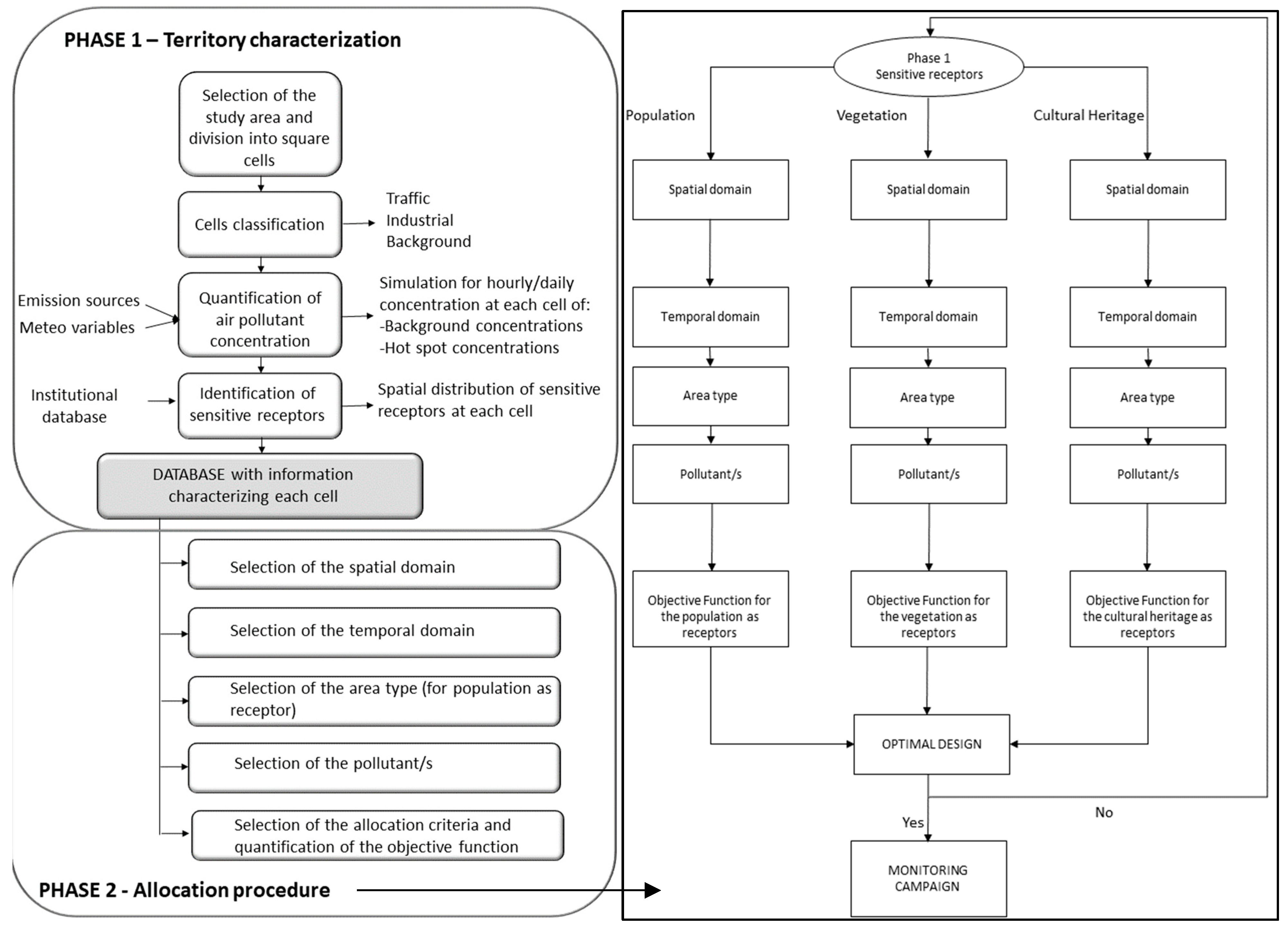
2.1. Description of the Methodology Development through Operations Research
x∈S
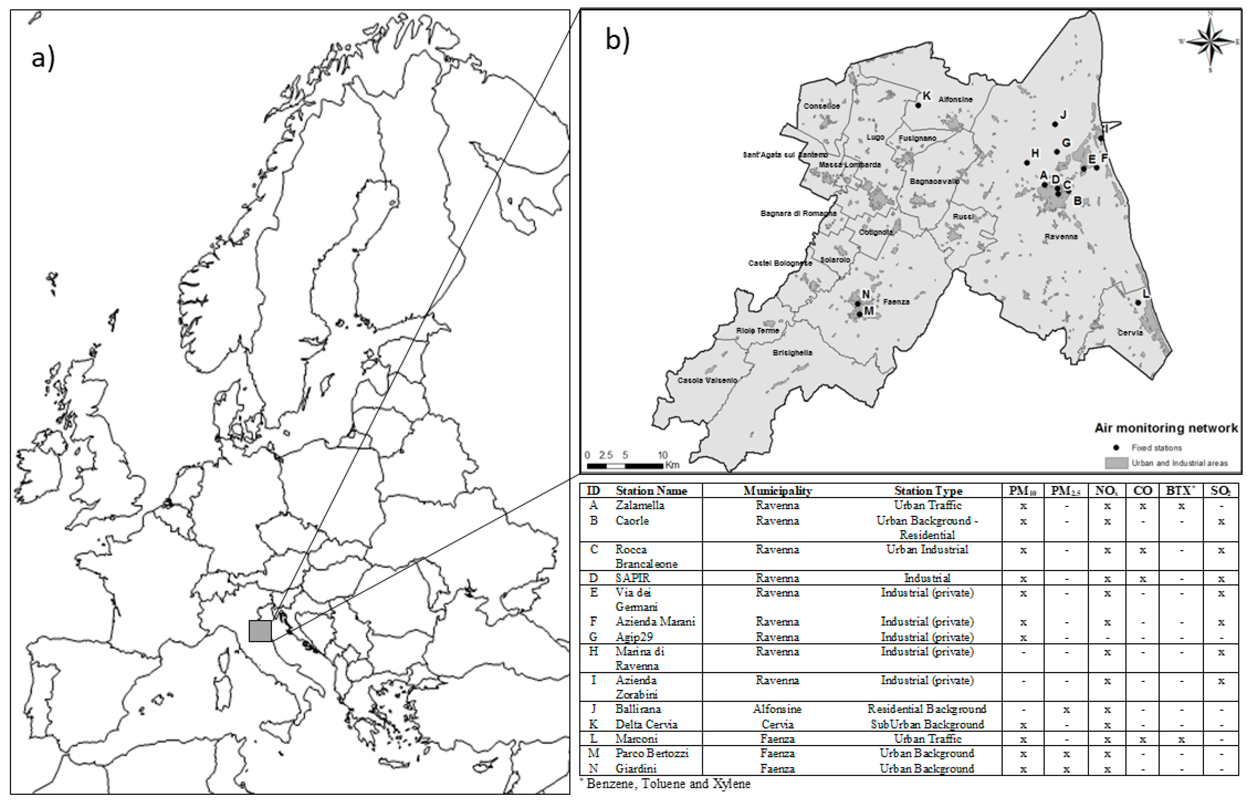
2.2. Description of the Study Area
3. Results and Discussion
3.1. Phase 1 Application
3.2. Phase 2 Application
3.2.1. Campaign n.1
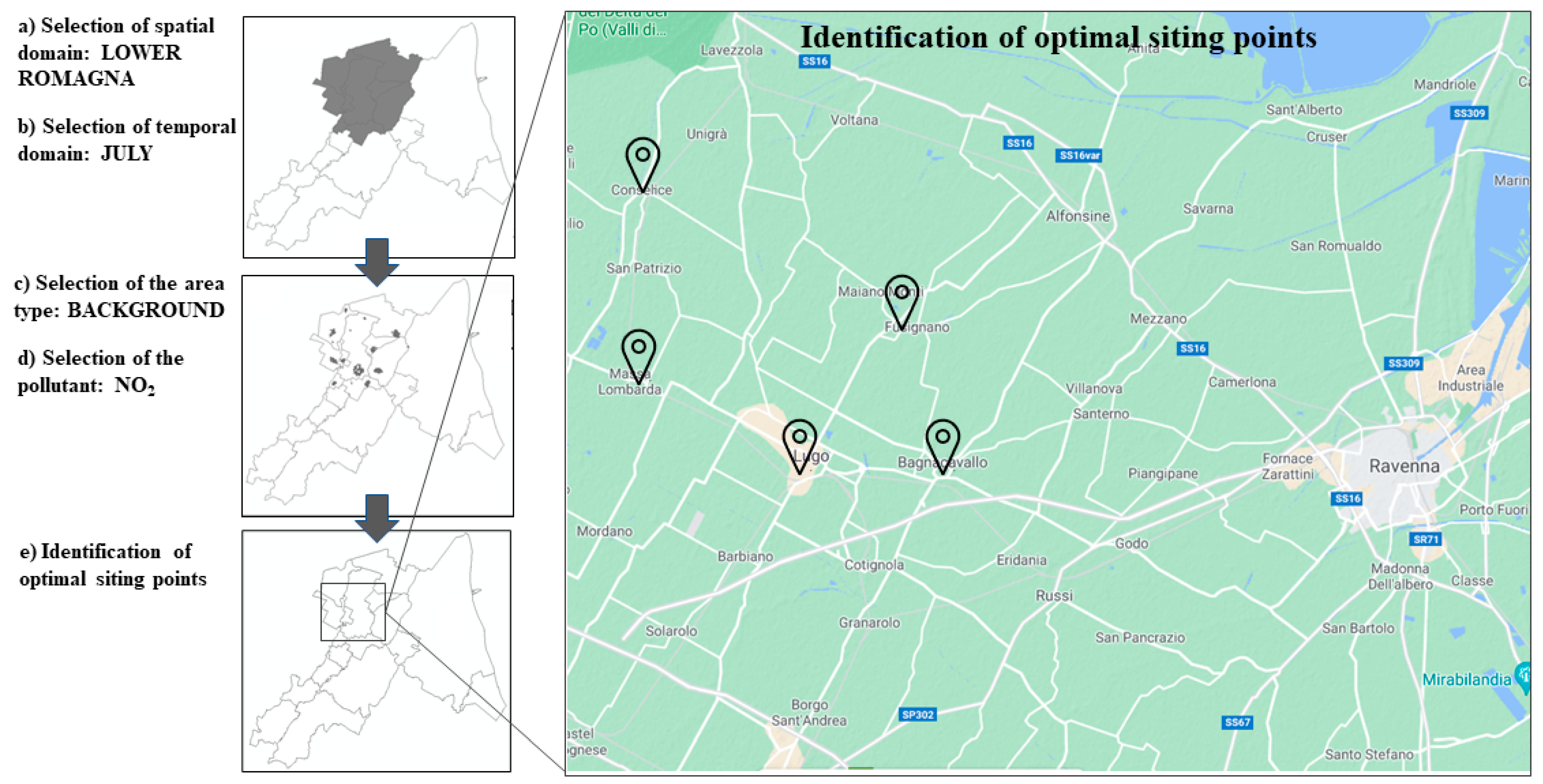
3.2.2. Campaign n.2
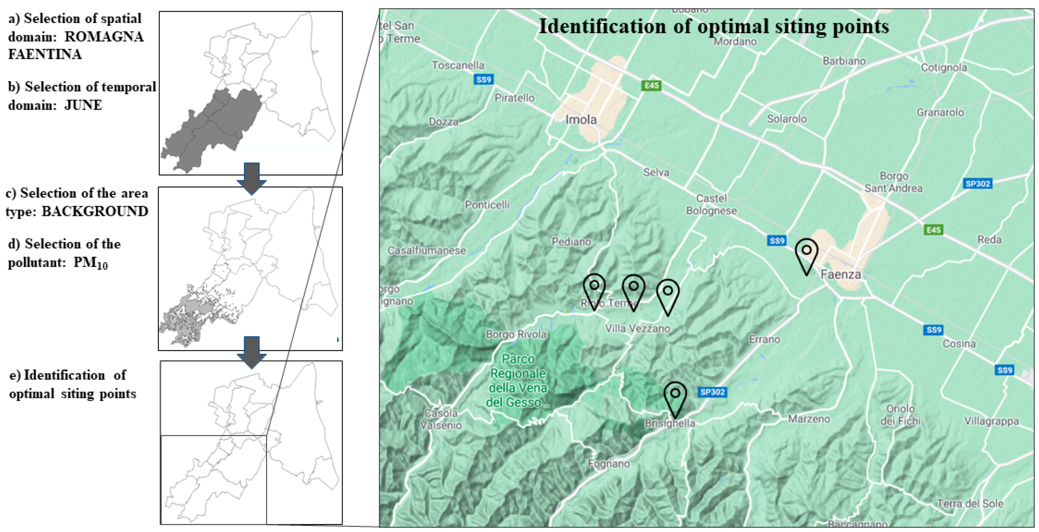
3.2.3. Campaign n.3
3.2.4. Campaign n.4
4. Conclusions
Supplementary Materials
Author Contributions
Funding
Institutional Review Board Statement
Informed Consent Statement
Data Availability Statement
Conflicts of Interest
References
- United Nations Economic and Social Council. Special Edition: Progress Towards the Sustainable Development Goals Report of the Secretary-General. 2019. Available online: https://undocs.org/E/2019/68 (accessed on 9 November 2020).
- USEPA. Ambient Air Quality Surveillance Regulations; USEPA: Washington, DC, USA, 1994.
- European Commission. Directive 2008/50/EC of the European Parliament and of the Council of 21 May 2008 on Ambient Air Quality and Cleaner Air for Europe; European Commission: Brussels, Belgium, 2008. [Google Scholar]
- Cohen, A.J.; Anderson, A.J.; Ostro, B.; Pandey, K.D.; Krzyzanowski, M.; Kuenzli, N.; Gutschmidt, K.; Pope, C.A.; Romieu, I.; Samet, J.M.; et al. Mortality Impacts of Urban Air Pollution; Taylor and Francis: New York, NY, USA, 2004. [Google Scholar]
- Araki, S.; Shima, M.; Yamamoto, K. Estimating historical PM2.5 exposures for three decades (1987–2016) in Japan using measurements of associated air pollutants and land use regression. Environ. Pollut. 2020, 263, 114476. [Google Scholar] [CrossRef] [PubMed]
- Zhang, F.; Shi, Y.; Fang, D.; Ma, G.; Nie, C.; Krafft, T.; He, L.; Wang, Y. Monitoring history and change trends of ambient air quality in China during the past four decades. J. Environ. Manag. 2020, 260, 110031. [Google Scholar] [CrossRef]
- Jimmink, B.; de Leeuw, F.; Noordijk, E.; Ostatnická, J.; Coòková, M. Reporting on Ambient Air Quality Assessment in the EU Member States; ETC/ACM: Bilthoven, The Netherlands, 2010. [Google Scholar]
- Hussein, T.; Saleh, S.; Dos Santos, V.; Abdullah, H.; Boor, B.E. Black Carbon and Particulate Matter Concentrations in Eastern Mediterranean Urban Conditions: An Assessment Based on Integrated Stationary and Mobile Observations. Atmosphere 2019, 10, 323. [Google Scholar] [CrossRef] [Green Version]
- Kerckhoffs, J.; Hoek, G.; Vlaanderen, J.; van Nunen, E.; Messier, K.; Brunekreef, B.; Gulliver, J.; Vermeulen, R. Robustness of intra urban land-use regression models for ultrafine particles and black carbon based on mobile monitoring. Environ. Res. 2017, 159, 500–508. [Google Scholar] [CrossRef]
- Crocchianti, S.; Del Sarto, S.; Ranalli, M.G.; Moroni, B.; Castellini, S.; Petroselli, C.; Cappelletti, D. Spatiotemporal correlation of urban pollutants by long-term measurements on a mobile observation platform. Environ. Pollut. 2021, 268, 115645. [Google Scholar] [CrossRef]
- Sim, S.; Jeong, S.; Park, H.; Park, C.; Kwak, K.-H.; Lee, S.-B.; Kim, C.H.; Lee, S.; Chang, J.S.; Kang, H.; et al. Co-benefit potential of urban CO2 and air quality monitoring: A study on the first mobile campaign and building monitoring experiments in Seoul during the winter. Atmos. Pollut. Res. 2020, 11, 1963–1970. [Google Scholar] [CrossRef]
- Liu, X.; Jayaratne, R.; Thai, P.; Kuhn, T.; Zing, I.; Christensen, B.; Lamont, R.; Dunbabin, M.; Zhu, S.; Gao, J.; et al. Low-cost sensors as an alternative for long-term air quality monitoring. Environ. Res. 2020, 185, 109438. [Google Scholar] [CrossRef] [PubMed]
- Andretta, M.; Coppola, F.; Pavlovic, A. New Technologies for Microclimatic and Indoor Air Quality Analysis for the Protection of Cultural Heritage: Case Studies of the Classense Library and “Tamo,” The Museum of Mosaics at Ravenna. In Advances in Applications of Industrial Biomaterials; Pellicer, E., Ed.; Springer: Cham, Switzerland, 2017; pp. 161–178. ISBN 9783319627670. [Google Scholar]
- Marinello, S.; Lolli, F.; Gamberini, R. Roadway tunnels: A critical review of air pollutant concentrations and vehicular emissions. Transp. Res. Part D Transp. Environ. 2020, 86, 102478. [Google Scholar] [CrossRef]
- Chen, S.; Broday, D.M. Re-framing the Gaussian dispersion model as a nonlinear regression scheme for retrospective air quality assessment at a high spatial and temporal resolution. Environ. Model. Softw. 2020, 125, 104620. [Google Scholar] [CrossRef]
- Righi, S.; Lucialli, P.; Pollini, E. Statistical and diagnostic evaluation of the ADMS-Urban model compared with an urban air quality monitoring network. Atmos. Environ. 2009, 43, 3850–3857. [Google Scholar] [CrossRef]
- Liao, H.-T.; Yau, Y.-C.; Huang, C.-S.; Chen, N.; Chow, J.C.; Watson, J.G.; Tsai, S.-W.; Chou, C.C.-K.; Wu, C.-F. Source apportionment of urban air pollutants using constrained receptor models with a priori profile information. Environ. Pollut. 2017, 227, 323–333. [Google Scholar] [CrossRef]
- Pirjola, L.; Paasonen, P.; Pfeiffer, D.U.; Hussein, T.; Hämeri, K.; Koskentalo, T.; Virtanen, A.; Rönkkö, T.; Keskinen, J.; Pakkanen, T.A. Dispersion of particles and trace gases nearby a city highway: Mobile laboratory measurements in Finland. Atmos. Environ. 2006, 40, 867–879. [Google Scholar] [CrossRef]
- Denby, W.P.; Ossenbruggen, P.J.; Members, A. Optimization of urban air monitoring networks. J. Environ. Eng. Div. 1974, 5, 577–591. [Google Scholar]
- Noll, K.E.; Miller, T.L.; Norco, J.E.; Raufer, R.K. An objective air monitoring site selection methodology for large point sources. Atmos. Environ. 1977, 11, 1051–1059. [Google Scholar] [CrossRef]
- Noll, K.E.; Mitsutomi, S. Design methodology for optimum dosage air monitoring site selection. Atmos. Environ. 1983, 17, 2583–2590. [Google Scholar] [CrossRef]
- Husain, T.; Khan, H.U. Shannon’s entropy concept in optimum air monitoring network design. Sci. Total Environ. 1983, 30, 181–190. [Google Scholar] [CrossRef]
- Husain, T.; Khan, S.M. Air monitoring network design using Fischer’s information measure—A case study. Atmos. Environ. 1983, 17, 2591–2598. [Google Scholar] [CrossRef]
- Modak, P.M.; Lohani, B.N. Optimization of ambient air quality monitoring networks. Environ. Monit. Assess. 1985, 5, 1–19. [Google Scholar] [CrossRef] [PubMed]
- Silva, C.; Quiroz, A. Optimization of the atmospheric pollution monitoring network at Santiago de Chile. Atmos. Environ. 2003, 37, 2337–2345. [Google Scholar] [CrossRef]
- Liu, M.K.; Avrin, J.; Pollack, R.I.; Behar, J.V.; McElroy, J.L. Methodology for designing air quality monitoring networks: I theorical aspects. Environ. Monit. Assess. 1986, 6, 1–11. [Google Scholar] [CrossRef]
- McElroy, J.L.; Behar, J.V.; Meyers, T.C.; Liu, M.K. Methodology for designing air quality monitoring networks: II. Application to Las Vegas, Nevada, for carbon monoxide. Environ. Monit. Assess. 1986, 6, 13–34. [Google Scholar] [CrossRef] [PubMed]
- Mofarrah, A.; Husain, T. A holistic approach for optimal design of air quality monitoring network expansion in an urban area. Atmos. Environ. 2010, 44, 432–440. [Google Scholar] [CrossRef]
- Righini, G.; Cappelletti, A.; Ciucci, A.; Cremona, G.; Piersanti, A.; Vitali, L.; Ciancarella, L. GIS based assessment of the spatial representativeness of air quality monitoring stations using pollutant emissions data. Atmos. Environ. 2014, 97, 121–129. [Google Scholar] [CrossRef]
- Langstaff, J.; Seigneur, C.; Mei-Kao, L.; Behar, J.; McElroy, J.L. Design of an optimum air monitoring network for exposure assessments. Atmos. Environ. 1967, 21, 1393–1410. [Google Scholar] [CrossRef]
- Trujillo-Ventura, A.; Ellis, J.H. Multiobjective air pollution monitoring network design. Atmos. Environ. Part. A Gen. Top. 1991, 25, 469–479. [Google Scholar] [CrossRef]
- Hwang, J.-S.; Chan, C.-C. Redundant Measurements of Urban Air Monitoring Networks in Air Quality Reporting. J. Air Waste Manag. Assoc. 1997, 47, 614–619. [Google Scholar] [CrossRef]
- Wang, C.; Zhao, L.; Sun, W.; Xue, J.; Xie, Y. Identifying redundant monitoring stations in an air quality monitoring network. Atmos. Environ. 2018, 190, 256–268. [Google Scholar] [CrossRef]
- Tseng, C.C.; Chang, N.-B. Assessing relocation strategies of urban air quality monitoring stations by GA-based compromise programming. Environ. Int. 2001, 26, 523–541. [Google Scholar] [CrossRef]
- Saisana, M.; Sarigiannis, D.; Chaloulakou, A.; Spyrellis, N. Air Quality Monitoring Design: Optimization of Pm2.5 Networks Using Satellite Observations. In Proceedings of the 7th Conference on Environmental Science and Technology, Syros, Greece, 3–6 September 2001; pp. 3–6. [Google Scholar]
- Sarigiannis, D.; Saisana, M. Multi-objective optimization of air quality monitoring. Environ. Monit. Assess. 2007, 136, 87–99. [Google Scholar] [CrossRef]
- Chow, J.C.; Engelbrecht, J.P.; Freeman, N.C.; Hashim, J.H.; Jantunen, M.; Michaud, J.-P.; De Tejada, S.S.; Watson, J.G.; Wei, F.; Wilson, W.E.; et al. Chapter one: Exposure measurements. Chemosphere 2002, 49, 873–901. [Google Scholar] [CrossRef]
- Chow, J.C.; Engelbrecht, J.P.; Watson, J.G.; Wilson, W.E.; Frank, N.H.; Zhu, T. Designing monitoring networks to represent outdoor human exposure. Chemosphere 2002, 49, 961–978. [Google Scholar] [CrossRef]
- Kanaroglou, P.S.; Jerrett, M.; Morrison, J.; Beckerman, B.; Arain, M.A.; Gilbert, N.; Brook, J.R. Establishing an air pollution monitoring network for intra-urban population exposure assessment: A location-allocation approach. Atmos. Environ. 2005, 39, 2399–2409. [Google Scholar] [CrossRef]
- Kao, J.-J.; Hsieh, M.-R. Utilizing multiobjective analysis to determine an air quality monitoring network in an industrial district. Atmos. Environ. 2006, 40, 1092–1103. [Google Scholar] [CrossRef]
- Venegas, L.E.; Mazzeo, N.A. Design methodology for background air pollution monitoring site selection in an urban area. Int. J. Environ. Pollut. 2003, 20, 185. [Google Scholar] [CrossRef]
- Elkamel, A.; Fatehifar, E.; Taheri, M.; Al-Rashidi, M.; Lohi, A. A heuristic optimization approach for Air Quality Monitoring Network design with the simultaneous consideration of multiple pollutants. J. Environ. Manag. 2008, 88, 507–516. [Google Scholar] [CrossRef] [PubMed]
- Hao, Y.; Xie, S. Optimal redistribution of an urban air quality monitoring network using atmospheric dispersion model and genetic algorithm. Atmos. Environ. 2018, 177, 222–233. [Google Scholar] [CrossRef]
- Gramsch, E.; Cereceda-Balic, F.; Oyola, P.; Vonbaer, D. Examination of pollution trends in Santiago de Chile with cluster analysis of PM10 and Ozone data. Atmos. Environ. 2006, 40, 5464–5475. [Google Scholar] [CrossRef]
- Chen, C.-H.; Liu, W.-L.; Chen, C.-H. Development of a multiple objective planning theory and system for sustainable air quality monitoring networks. Sci. Total Environ. 2006, 354, 1–19. [Google Scholar] [CrossRef]
- Ainslie, B.; Reuten, C.; Steyn, D.G.; Le, N.D.; Zidek, J.V. Application of an entropy-based Bayesian optimization technique to the redesign of an existing monitoring network for single air pollutants. J. Environ. Manag. 2009, 90, 2715–2729. [Google Scholar] [CrossRef]
- Mazzeo, N.; Venegas, N.M.A.L. Development and Application of a Methodology for Designing a Multi-Objective and Multi-Pollutant Air Quality Monitoring Network for Urban Areas. Air Quality 2010. [Google Scholar] [CrossRef] [Green Version]
- Alsahli, M.M.; Al-Harbi, M. Allocating optimum sites for air quality monitoring stations using GIS suitability analysis. Urban. Clim. 2018, 24, 875–886. [Google Scholar] [CrossRef]
- Munir, S.; Mayfield, M.; Coca, D.; Jubb, S.A. Structuring an integrated air quality monitoring network in large urban areas—Discussing the purpose, criteria and deployment strategy. Atmos. Environ. X 2019, 2, 100027. [Google Scholar] [CrossRef]
- Lolli, F.; Ishizaka, A.; Gamberini, R. New AHP-based approaches for multi-criteria inventory classification. Int. J. Prod. Econ. 2014, 156, 62–74. [Google Scholar] [CrossRef] [Green Version]
- Lolli, F.; Balugani, E.; Ishizaka, A.; Gamberini, R.; Butturi, M.A.; Marinello, S.; Rimini, B. On the elicitation of criteria weights in PROMETHEE-based ranking methods for a mobile application. Expert Syst. Appl. 2019, 120, 217–227. [Google Scholar] [CrossRef] [Green Version]
- Jahan, A.; Edwards, K.L.; Bahraminasab, M. Multi-criteria decision-making for materials selection. In Multi-Criteria Decision Analysis for Supporting the Selection of Engineering Materials in Product Design; Elsevier BV: Amsterdam, The Netherlands, 2016; pp. 63–80. [Google Scholar]
- ISTAT. Population Census. Available online: https://www.istat.it/it/archivio/104317#accordions (accessed on 4 May 2020).
- Andretta, M.; Leonzio, B.; Lucialli, P.; Righi, S. Application of the ISCST3 model to an industrial area: Comparison between predicted and observed concentrations. Water Pollut. VIII Model. Monit. Manag. 2006, 91, 187–195. [Google Scholar] [CrossRef] [Green Version]
- Bonafè, G.; Minguzzi, E.; Stortini, M.; Deserti, M. Il Sistema Modellistico NINFA+PESCO per la Valutazione e la Previsione della Qualità dell’Aria in Emilia-Romagna; Arpae Emilia-Romagna: Bologna, Italy, 2011. [Google Scholar]
- Bonafè, G.; Stortini, M.; Minguzzi, E.; Deserti, M. Postprocessing of a CTM with Observed Data: Downscaling, Unbiasing and Estimation of the Subgrid Scale Pollution Variability. In Proceedings of the 14th International Conference on Harmonisation within Atmospheric Dispersion Modelling for Regulatory Purposes, Kos, Greece, 2–6 October 2001. [Google Scholar]
- Arpae Pesco Model. Available online: https://github.com/ARPA-SIMC/pesco (accessed on 9 December 2019).
- CERC ADMS-URBAN—User Guide. 2020. Available online: https://www.cerc.co.uk/environmental-software/assets/data/doc_userguides/CERC_ADMS-Urban5.0_User_Guide.pdf (accessed on 4 July 2021).
- Righi, S.; Farina, F.; Marinello, S.; Andretta, M.; Lucialli, P.; Pollini, E. Development and evaluation of emission disaggregation models for the spatial distribution of non-industrial combustion atmospheric pollutants. Atmos. Environ. 2013, 79, 85–92. [Google Scholar] [CrossRef]
- Karppinen, A.; Kukkonen, J.; Elolähde, T.; Konttinen, M.; Koskentalo, T. A modelling system for predicting urban air pollution: Comparison of model predictions with the data of an urban measurement network in Helsinki. Atmos. Environ. 2000, 34, 3735–3743. [Google Scholar] [CrossRef]
- Kousa, A.; Kukkonen, J.; Karppinen, A.; Aarnio, P.; Koskentalo, T. Statistical and diagnostic evaluation of a new-generation urban dispersion modelling system against an extensive dataset in the Helsinki area. Atmos. Environ. 2001, 35, 4617–4628. [Google Scholar] [CrossRef]
- Spezzano, P. Mapping the susceptibility of UNESCO World Cultural Heritage sites in Europe to ambient (outdoor) air pollution. Sci. Total Environ. 2021, 754, 142345. [Google Scholar] [CrossRef] [PubMed]
- Di Turo, F.; Proietti, C.; Screpanti, A.; Fornasier, M.F.; Cionni, I.; Favero, G.; De Marco, A. Impacts of air pollution on cultural heritage corrosion at European level: What has been achieved and what are the future scenarios. Environ. Pollut. 2016, 218, 586–594. [Google Scholar] [CrossRef]
- Emilia-Romagna, R. CMS (Content Management System) GIS with Data on the Spatial Distribution of Vegetation. Available online: http://www.mokagis.it/html/applicazioni_mappe.asp (accessed on 4 May 2020).
- MIBACT. Territorial Information System to Support the Protection of Cultural Heritage. Available online: http://www.cartadelrischio.it/ (accessed on 4 May 2020).
- Lozano, A.; Usero, J.; Vanderlinden, E.; Raez, J.; Contreras, J.; Navarrete, B. Air quality monitoring network design to control nitrogen dioxide and ozone, applied in Malaga, Spain. Microchem. J. 2009, 93, 164–172. [Google Scholar] [CrossRef]
- Larsen, R.I.; Zimmer, C.E.; Lynn, D.A.; Blemel, K.G. Analyzing Air Pollutant Concentration and Dosage Data. J. Air Pollut. Control Assoc. 1967, 17, 85–93. [Google Scholar] [CrossRef] [PubMed]
- Negri, A.; Sozzi, R. Optimization criteria in network configuration for air quality monitoring: Analysis of available facilities and possible development lines. Environ. Softw. 1988, 3, 174–179. [Google Scholar] [CrossRef]
- Sajani, S.Z.; Scotto, F.; Lauriola, P.; Galassi, F.; Montanari, A. Urban air pollution monitoring and correlation properties between fixed-site stations. J. Air Waste Manag. Assoc. 2004, 54, 1236–1241. [Google Scholar] [CrossRef] [PubMed] [Green Version]
- Lee, T.D.; Graves, R.J.; McGinnis, L.F. A Procedure for Air Monitoring Instrumentation Location. Manag. Sci. 1978, 24, 1451–1461. [Google Scholar] [CrossRef]
- Corti, S.; Senatore, S. Project of an Air Quality Monitoring Network for Industrial Site in Italy. Environ. Monit. Assess. 2000, 65, 109–117. [Google Scholar] [CrossRef]
- Munshi, U.; Patil, R.S. A method for selection of air quality monitoring sites for multiple sources. Atmos. Environ. 1982, 16, 1915–1918. [Google Scholar] [CrossRef]
- Kumar, N.; Nixon, V.; Sinha, K.; Jiang, X.; Ziegenhorn, S.; Peters, T. An optimal spatial configuration of sample sites for air pollution monitoring. J. Air Waste Manag. Assoc. 2009, 59, 1308–1316. [Google Scholar] [CrossRef] [PubMed] [Green Version]
- Ott, W.R.; Thorn, G.C. Air Pollution Index Systems in the United States and Canada. J. Air Pollut. Control. Assoc. 1976, 26, 460–470. [Google Scholar] [CrossRef] [Green Version]
- Arpae Emilia Romagna. Definizione di un Indice di Qualità dell’Aria per l’Emilia-Romagna; Arpae Emilia Romagna: Bologna, Italy, 2008. [Google Scholar]
- ARPAV. Ottimizzazione Della Rete Regionale di Controllo Della Qualità dell’Aria del Veneto e Mappatura di Aree Remote; ARPAV: Padova, Italy, 2006. [Google Scholar]
- ISPRA. Valutazione Degli Effetti dell’Inquinamento Atmosferico sui beni Culturali Architettonici di Roma; ISPRA: Rome, Italy, 2011.
- Lipfert, F.W. Dry Deposition Velocity as an Indicator for SO2 Damage to Materials. JAPCA 1989, 39, 446–452. [Google Scholar] [CrossRef] [Green Version]
- Gulia, S.; Prasad, P.; Goyal, S.; Kumar, R. Sensor-based Wireless Air Quality Monitoring Network (SWAQMN)—A smart tool for urban air quality management. Atmos. Pollut. Res. 2020, 11, 1588–1597. [Google Scholar] [CrossRef]
- Singla, S.; Bansal, D.; Misra, A.; Raheja, G. Towards an integrated framework for air quality monitoring and exposure estimation—A review. Environ. Monit. Assess. 2018, 190, 562. [Google Scholar] [CrossRef] [PubMed]
- EPA (Environmental Protection Agency). SPECIATE 4.4 Database. Available online: https://www.epa.gov/ (accessed on 1 June 2015).


| Authors | Objectives | Variable/s of Action | Constraint/s | Sensitive Receptor/s |
|---|---|---|---|---|
| [19] | Number and placement | Pollution dosage | Exposure time to pollutant | Population |
| [20] | Maximum concentration values | Single source, pollutant and meteorological conditions | ||
| [21] | Exceeding the law limits | Number of points defined before single pollutant | ||
| [22,23,24,25] | Information associated to the signal | Previously measured data | ||
| [26,27,28,29] | Spheres of influence | Data from air quality dispersion model | ||
| [30] | Pollution exposure gradient | Previously measured data | ||
| [31] | Weighing function of maximum concentration values, exceeding the law limits, cost of the network and data validation | Previously measured data Economic aspect | ||
| [32,33] | Site redundancy | Previous network | ||
| [34] | Exceeding the law limits Protection capability Average daily concentration | Data from air quality dispersion model | ||
| [35,36] | Information gain | Adding new stations | ||
| [37,38,39] | Pollution exposure | Single pollutant Previously measured data | ||
| [40] | Overall function of maximum concentration values, maximum dosage, maximum network coverage, maximum population protection | Applied to pollution from industrial districts | ||
| [41,42,43] | Exceeding the law limits | Number of points defined before Number of points defined on the economic basis | ||
| [44] | Cluster analysis procedure | Previously measured data | ||
| [45] | Multiple criteria | Available budget | ||
| [46] | Entropy-based Bayesian optimizing approach | Available budget | ||
| [47] | Detection of higher pollutant concentrations “Protection capability” for areas with higher population density | Distribution of population, budget | ||
| [48] | Population and emission sources | |||
| [49] | Pollution exposure |
| Allocation Criteria | Sensitive Receptors | Note |
|---|---|---|
| Individual exposition to the i-th pollutant in the k-th cell [μg·m−3·h] | Population Vegetation | Quantifies the exposure of an individual to a specific outdoor pollutant [20,66,67,68] |
| Overall exposition to the i-th pollutant in the k-th cell [μg·m−3·h·n] | Population | Quantifies the overall exposure of all individuals present in a given cell [30,40] |
| Overall risk to all thepollutants in the k-th cell [μg·m−3·h] | Population Vegetation | Quantifies the individual risk as the contribution of all the considered pollutants |
| Correlation between simulated and measured data of the i-th pollutant in the k-th cell | Population | Identifies areas with a good match between the measured data from fixed air quality monitoring stations and concentration data estimated [35,69] |
| Exceedance of the legal limits of the i-th pollutant in the k-th cell [n.] | Population Vegetation | Identifies the probability of exceeding the legal limits for a specific pollutant [24,31,34,35,36,41,42,47,68,70] |
| Maximum concentration value of the i-th pollutant in the k-th cell [μg·m−3] | Population Vegetation | Identifies the probability of measuring an elevated concentration value for a specific pollutant [34,71,72] |
| Minimum index of agreement (IOA) for the i-th pollutant in the k-th cell | Population | Assess how the values simulated by the model deviate from the values measured by the fixed air monitoring stations |
| Minimum index of agreement normalized with the resident population (IOAPr) for the i-th pollutant in the k-th cell | Population | Assess how the values simulated by the model deviate from the values measured by the fixed air monitoring stations, considering also the presence of resident population. |
| Maximum concentration gradient for the i-th pollutant in the k-th cell | Population | Assesses how changing the concentration field at a specific point compared to neighboring points [30,39,73] |
| Maximum air quality index in the k-th cell | Population | Assesses the contribution of all the pollutants at the same time [24,74,75] |
| Minimum concentration difference in the k-th cell | Population | Assesses how changing the concentration field at a specific point compared to whole study area [31,73] |
| Maximum pollutant deposition in the k-th cell | Vegetation | Assess the total deposition of the selected pollutants [76] |
| Maximum PM10 deposition in the k-th cell | Vegetation | Assess the total deposition of the selected pollutants [76] |
| Maximum damage index in the k-th cell | Physical cultural heritage | Assess the total damage due to erosion blackening pollutants [76,77,78] |
| Fixed Air Quality Monitoring Stations | Measured MEAN (µg/m3) | Predicted MEAN (µg/m3) | CORR | NMSE | FA2 | FB | IOA |
|---|---|---|---|---|---|---|---|
| NO2 | |||||||
| B—Caorle | 25.35 | 24.49 | 0.81 | 0.20 | 0.85 | 0.03 | 0.90 |
| C—Rocca Brancaleone | 32.23 | 32.15 | 0.77 | 0.13 | 0.92 | 0.00 | 0.86 |
| D—SAPIR | 47.12 | 26.64 | 0.63 | 0.43 | 0.58 | 0.56 | 0.62 |
| F—Azienda Marani | 32.81 | 26.26 | 0.60 | 0.46 | 0.67 | 0.22 | 0.67 |
| H—Marina di Ravenna | 21.77 | 18.90 | 0.65 | 0.36 | 0.73 | 0.14 | 0.78 |
| I—Azienda Zorabini | 15.72 | 21.16 | 0.57 | 0.75 | 0.51 | 0.29 | 0.71 |
| J—Ballirana | 22.63 | 20.10 | 0.80 | 0.18 | 0.90 | 0.12 | 0.88 |
| L—Marconi | 34.20 | 29.98 | 0.98 | 0.03 | 0.99 | 0.13 | 0.95 |
| M—Parco Bertozzi | 28.54 | 28.60 | 0.87 | 0.14 | 0.90 | 0.00 | 0.93 |
| N—Giardini | 21.45 | 21.27 | 0.94 | 0.06 | 0.95 | 0.01 | 0.97 |
| PM10 | |||||||
| B—Caorle | 30.83 | 35.6 | 0.58 | 0.30 | 81.36 | −0.14 | 0.72 |
| C—Rocca Brancaleone | 29.89 | 34.09 | 0.67 | 0.16 | 89.75 | −0.13 | 0.79 |
| D—SAPIR | 44.77 | 25.71 | 0.59 | 0.72 | 63.46 | 0.54 | 0.52 |
| F—Azienda Marani | 26.66 | 21.00 | 0.60 | 0.29 | 83.71 | 0.24 | 0.79 |
| L—Marconi | 30.90 | 30.39 | 0.67 | 0.15 | 94.66 | 0.02 | 0.79 |
| M—Parco Bertozzi | 23.64 | 27.25 | 0.68 | 0.27 | 88.14 | −0.14 | 0.78 |
| N—Giardini | 25.05 | 32.04 | 0.61 | 0.32 | 78.33 | −0.24 | 0.69 |
| Decision Criteria | Example n.1 | Example n.2 | Example n.3 | Example n.4 |
| Spatial domain | Territory of the municipality of Ravenna | Territory of the municipality’s union of the lower Romagna | Territory of the municipality’s union of the Romagna Faentina | Territory of the municipality of Ravenna |
| Temporal domain | Month of October | Month of July | Month of June | Month of December |
| Area type | Urban traffic (T) | Urban background residential (BU-Res) | Rural background (BR) | All |
| Pollutant | NO2 | NO2 | PM10 | PM10 |
| Allocation criteria and objective function | Overall exposition to NO2 of the residential population | Maximum concentration values of NO2 | Maximum PM10 deposition | Maximum damage index |
Publisher’s Note: MDPI stays neutral with regard to jurisdictional claims in published maps and institutional affiliations. |
© 2021 by the authors. Licensee MDPI, Basel, Switzerland. This article is an open access article distributed under the terms and conditions of the Creative Commons Attribution (CC BY) license (https://creativecommons.org/licenses/by/4.0/).
Share and Cite
Marinello, S.; Andretta, M.; Lucialli, P.; Pollini, E.; Righi, S. A Methodology for Designing Short-Term Stationary Air Quality Campaigns with Mobile Laboratories Using Different Possible Allocation Criteria. Sustainability 2021, 13, 7481. https://doi.org/10.3390/su13137481
Marinello S, Andretta M, Lucialli P, Pollini E, Righi S. A Methodology for Designing Short-Term Stationary Air Quality Campaigns with Mobile Laboratories Using Different Possible Allocation Criteria. Sustainability. 2021; 13(13):7481. https://doi.org/10.3390/su13137481
Chicago/Turabian StyleMarinello, Samuele, Massimo Andretta, Patrizia Lucialli, Elisa Pollini, and Serena Righi. 2021. "A Methodology for Designing Short-Term Stationary Air Quality Campaigns with Mobile Laboratories Using Different Possible Allocation Criteria" Sustainability 13, no. 13: 7481. https://doi.org/10.3390/su13137481