
The Italian National Strategy for Inner Areas (SNAI): A Critical Analysis of the Indicator Grid


Abstract
:1. Introduction
2. The National Strategy for Inner Areas (SNAI)
2.1. Contents and Objectives
- Significantly distant from the main centers offering essential welfare services (education, healthcare, and mobility);
- Endowed with significant environmental resources (water resources, agricultural systems, natural and human-made environment) and cultural resources (historical villages, craft centers);
- A diversified territory as a result of the different natural systems’ dynamics and human activity.
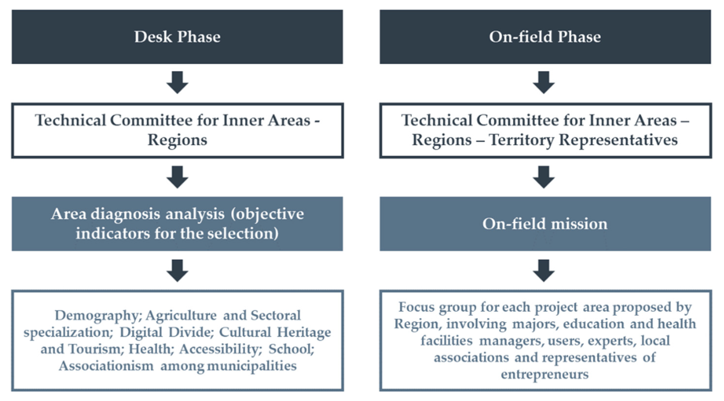
- A former desk phase for the area diagnosis. It involves the Technical Committee in assessing the various proposals to inner area projects submitted by the reference regions. This diagnosis process rests on an Indicator Grid, defined for the whole national territory, as an objective tool to evaluate the candidate areas’ conditions;
- A latter on-field phase. At this point, the key elements that emerged from the area diagnosis are improved and enriched thanks to the direct interaction with the territory and its community.
2.2. An Indicator Grid for the “Area Diagnosis” Process
- Main characteristics;
- Demography;
- Agriculture and sectoral specialization;
- Digital divide;
- Cultural heritage and tourism;
- Health;
- Accessibility;
- School;
- Cooperation among municipalities.
- A large number of indicators makes it hard to collect the necessary information to update the Grid or apply it at the municipality level to understand the power balance among municipalities in the same project area. The SNAI Grid, indeed, consists of 161 indicators;
- The difficulty of collecting all the data. The Grid, in its current state, requires much information which is not easily accessible and needs cooperation among different public institutions. The related required efforts, if appropriate for the project areas selection in the SNAI launch phase, can prevent the Grid’s extensive use as practical support for decisions;
- A large amount of information to manage and the difficulties in accessing data sources hinder comprehensive qualitative analysis processes geared towards better investigating relations among different variables and delving into territorial dynamics. Indeed, without qualitative interpretation, flanking the objective qualitative assessment, the Indicator Grid boils down to an uncritical collection of variables, making limited sense when dealing with planning issues, widely acknowledged as wicked problems [23];
- The selected indicators display some biases emerging when dealing with the cultural heritage and tourism section. Indeed, the indicators composing this section of the Grid reflect a partial and limited vision of cultural heritage as a tourism attraction. In more detail, all the indicators belonging to the Grid’s sections are only measures of tourist flows related to cultural heritage. On the contrary, there is no indicator considering built heritage use and conservation state or describing the ongoing enhancement initiatives in the inner areas. Again, the cooperation among municipalities only includes indicators concerning the relations among municipalities, without considering other kinds of synergies within local communities, which can play a fundamental role in pursuing the place-based approach at SNAI’s core [24];
- Some Grid indicators are conceived for the inner areas’ territorial dimension and cannot be applied at the municipality scale.
3. A Hybrid Methodological Approach towards SNAI Indicator Grid Review
- On the one hand, to discard the indicators referring to the inner area territorial scale, thus allowing turning the SNAI Grid into a decision support tool applicable at the municipality scale and, therefore, able to provide an in-depth understanding of territorial dynamics and power relations among municipalities belonging to the same inner areas. Indeed, the Grid includes several indicators—i.e., the number of municipalities in 2011—which lose their meaning when defined at the municipal scale.
- On the other hand, to reduce the redundancy of the Grid, intended as the presence of the same piece of information in two different indicators [27,28]. In more detail, this is mainly conducted by addressing temporal redundancy and, thus, rejecting the indicators occurring twice with a different time horizon, when their combined use does not pitch in the interpretation of the phenomena under investigation. Indeed, the latest version of the Grid, obtained by updating the first one issued in 2014, displays the addition of several indicators, equal to the already existing ones, but with a different time reference.
- If , the variables X and Y are weakly correlated;
- If , the variables X and Y are moderately correlated;
- If , the variables X and Y are markedly correlated;
- If , the variables X and Y are strongly correlated.
4. Application of the Hybrid Methodological Approach to the SNAI Indicator Grid
4.1. The “Demography” Section
4.1.1. Phase 1: Critical Analysis of the Indicator Set
4.1.2. Phase 2: Performing a Correlation Analysis of Selected Indicators
4.1.3. Phase 3: Critical Interpretation of the Associations and PCA Application
- B.4 (Percentage of population aged 0–16 in 2017) is moderately correlated with b.5 (Percentage of population aged 17–34 in 2017) and markedly correlated with b.6 (Percentage of population over 65 in 2017); b.5 and b.6 are strongly correlated;
- b.10 (Percentage variation in the resident population between 2001 and 2011) is strongly correlated with b.9 (Percentage variation in the resident population between 1971 and 2011) and markedly correlated with b.11 (Percentage variation in the resident population between 2011 and 2017); at the same time, b.9 and b.11 are markedly correlated.
4.2. The “Agriculture and Sectoral Specialization” Section
4.2.1. Phase 1: Critical Analysis of the Indicator Set
4.2.2. Phase 2: Performing a Correlation Analysis of Selected Indicators
4.2.3. Phase 3: Critical Interpretation of the Associations and PCA Application
- c.1 (Percentage of UAA in 2010) and c.2 (Percentage variation in the UAA between 1982 and 2010) are strongly correlated, and they are both markedly correlated with c.3 (Percentage variation in the UAA between 2000 and 2010);
- c.15 (Percentage of UAA in 2010) and c.13 (Percentage variation in the UAA between 1982 and 2010) are strongly correlated.
4.3. The “Cultural Heritage and Tourism” Section
4.3.1. Phase 1: Critical Analysis of the Indicator Set
4.3.2. Phase 2: Performing a Correlation Analysis of Selected Indicators
4.3.3. Phase 3: Critical Interpretation of the Associations and PCA Application
- e.7 (Number of visitors in 2015) and e.8 (Number of visitors per 1000 inhabitants in 2015) are strongly correlated;
- e.11 (Tourism rate—number of presences per 1000 inhabitants in 2016) is strongly correlated with e.10 (Accommodation rate—bed places for 1000 inhabitants in 2016) and markedly correlated both with e.13 (Arrivals in 2016) and e.16 (Presences in 2016);
- e.16 (Presences in 2016) is strongly correlated with e.13 (Arrivals in 2016);
- e.17 (Percentage variation in presences between 2014 and 2016) is strongly correlated with e.14 (Percentage variation in arrivals between 2014 and 2016);
- e.18 (Percentage of presences in hotel facilities in 2016), e.19 (Percentage of presences in extra-hotel facilities in 2016), e.20 (Percentage of arrivals in hotel facilities in 2016), and e.21 (Percentage of arrivals in extra-hotel facilities in 2016) are strongly correlated with each other.
4.4. The “Cooperation among Municipalities” Section
5. Results, Discussion, and Further Developments
- Gaining a comprehensive understanding of territorial dynamics and power balances thanks to the data related to each Grid section and available for each municipality within each inner area;
- Defining interventions and efficiently allocating resources according to the actual inner areas’ needs;
- Prioritizing actions within a project area or selecting additional areas for SNAI relaunch;
- Providing a good reference for setting goals to be reached and for their monitoring in performance terms.
Author Contributions
Funding
Data Availability Statement
Conflicts of Interest
Appendix A

| A. Main Characteristics | |||||
| a.1 | Number of municipalities in 2011 | a.2 | of which: inner areas | a.3 | of which: peripheral and ultra-peripheral areas |
| a.4 | Resident population in 2011 | a.5 | of which: inner areas | a.6 | of which: peripheral and ultra-peripheral areas |
| a.7 | of which: percentage inner areas | a.8 | of which: percentage peripheral and ultra-peripheral areas | a.9 | Number of municipalities in 2017 |
| a.10 | of which: inner areas | a.11 | of which: peripheral and ultra-peripheral areas | a.12 | Resident population in 2017 |
| a.13 | of which: inner areas | a.14 | of which: peripheral and ultra-peripheral areas | a.15 | of which: percentage inner areas |
| a.16 | of which: percentage peripheral and ultra-peripheral areas | a.17 | Total area in km2 | a.18 | Density per km2 |
| B. Demography | |||||
| b.1 | Percentage of population aged 0–16 in 2011 | b.2 | Percentage of population aged 17–34 in 2011 | b.3 | Percentage of population aged 65+ in 2011 |
| b.4 | Percentage of population aged 0–16 in 2017 | b.5 | Percentage of population aged 17–34 in 2017 | b.6 | Percentage of population aged 65+ in 2017 |
| b.7 | Percentage of foreign residents in 2011 | b.8 | Percentage of foreign residents in 2017 | b.9 | Percentage variation in the resident population between 1971 and 2011 |
| b.10 | Percentage variation in the resident population between 2001 and 2011 | b.11 | Percentage variation in the resident population between 2011 and 2017 | b.12 | Percentage variation in the resident foreign population between 2001 and 2011 |
| b.13 | Percentage variation in the resident foreign population between 2011 and 2017 | ||||
| C. Agriculture and Sectoral Specialization | |||||
| c.1 | Percentage of utilized agricultural area (UAA) in 2010 | c.2 | Percentage variation in the UAA between 1982 and 2010 | c.3 | Percentage variation in the UAA between 2000 and 2010 |
| c.4 | Percentage of farmers aged up to 39 years on the total of farmers in 2010 | c.5 | Percentage variation in the number of farmers aged up to 39 between 2000 and 2010 | c.6 | Percentage of part-time farmers in 2010 |
| c.7 | Percentage variation in the number of part-time farmers between 2000 and 2010 | c.8 | Percentage of protected area | c.9 | Percentage of forest area |
| c.10 | Importance index for the agricultural sector in 2001 | c.11 | Importance index for the agri-food industry in 2001 | c.12 | Importance index for the total agri-food sector in 2001 |
| c.13 | Importance index for the agricultural sector in 2011 | c.14 | Importance index for the agri-food industry in 2011 | c.15 | Importance index for the total agri-food sector in 2011 |
| c.16 | Incidence of farms with DOP and/or IGP products | c.17 | Breeding farms on the total of farms | c.18 | Percentage of permanent meadows and pastors on the total UAA |
| c.19 | Breeding farms size (UBA) | c.20 | Percentage of farms with standard production of EUR 25,000 | c.21 | Specialization index for the manufacturing sector in 2009 |
| c.22 | Specialization index for the energy, gas, and water sector in 2009 | c.23 | Specialization index for the construction sector in 2009 | c.24 | Specialization index for the trade sector in 2009 |
| c.25 | Specialization index for the other services sector in 2009 | c.26 | Number of companies per 1000 inhabitants | c.27 | Companies’ stock growth rate in 2013 |
| c.28 | Percentage of foreign companies | ||||
| D. Digital Divide | |||||
| d.1 | Percentage of population reached by fixed-line broadband higher than 2 Mbps and lower than 20 Mbps | d.2 | Percentage of population reached by fixed-line broadband higher than 20 Mbps | d.3 | Fixed-line digital divide |
| d.4 | Fixed-line and mobile-line digital divide | ||||
| E. Cultural Heritage and Tourism | |||||
| e.1 | Number of state and non-state cultural sites in 2012 | e.2 | Number of not accessible state and non-state cultural sites in 2012 | e.3 | Number of visitors in 2012 |
| e.4 | Percentage of paying visitors in 2012 | e.5 | Number of visitors per 1000 inhabitants in 2012 | e.6 | Number of state and non-state cultural sites in 2015 |
| e.7 | Number of visitors in 2015 | e.8 | Number of visitors per 1000 inhabitants in 2015 | e.9 | Accommodation rate—bed places for 1000 inhabitants in 2012 |
| e.10 | Accommodation rate—bed places for 1000 inhabitants in 2016 | e.11 | Tourism rate—number of presences per 1000 inhabitants in 2016 | e.12 | Arrivals in 2014 |
| e.13 | Arrivals in 2016 | e.14 | Percentage variation in arrivals between 2014 and 2016 | e.15 | Presences in 2014 |
| e.16 | Presences in 2016 | e.17 | Percentage variation in presences between 2014 and 2016 | e.18 | Percentage of presences in hotel facilities in 2016 |
| e.19 | Percentage of presences in extra-hotel facilities in 2016 | e.20 | Percentage of arrivals in hotel facilities in 2016 | e.21 | Percentage of arrivals in extra-hotel facilities in 2016 |
| F. Health | |||||
| f.1 | Ambulatory specialization—medical services provide per 1000 residents | f.2 | Hospitalization rate (LEA = 170) | f.3 | Over 75 hospitalization rate |
| f.4 | Avoidable hospitalization rate (LEA = 570) | f.5 | Percentage of over 65 residents treated by integrated care home assistance (ADI) | f.6 | Number of births in which the first visit is conducted after the 12th week of gestation |
| f.7 | Time (minutes) passing between the first call and the rescue vehicles’ arrival | f.8 | Average number of patients per doctor in 2012 | f.9 | Average number of patients per pediatrician in 2012 |
| G. Accessibility | |||||
| g.1 | Municipalities’ average distance in minutes from the nearest center | g.2 | Municipalities’ average distance in minutes from the nearest center, weighted on the population | g.3 | LPT road services offer to connect with the regional centers |
| g.4 | LPT road services offer to connect with the local centers | g.5 | Percentage of population residing within 15 min from the reference railway station | g.6 | Percentage of population residing between 15 and 30 min from the reference railway station |
| g.7 | Regional rail services’ intensity related to the resident population able to access it in less than 15 min by car | g.8 | Regional rail services’ intensity related to the resident population able to access it in less than 30 min by car | g.9 | Percentage of population residing within 15 min from the reference highway tollbooth |
| g.10 | Percentage of population residing between 15 and 30 min from the reference highway tollbooth | g.11 | Percentage of population residing within 30 min from the reference airport | g.12 | Percentage of population residing within 30 min from the reference airport |
| g.13 | Synthetic indicator of road accessibility for the goods in the reference labor market areas | ||||
| H. School | |||||
| h.1 | Average number of facilities per educational institution | h.2 | Number of primary schools | h.3 | Percentage of municipalities with primary schools |
| h.4 | Average number of students per secondary school | h.5 | Percentage of international students in primary schools | h.6 | Ratio between children between disabilities and support teachers in primary schools |
| h.7 | Percentage of students resident in their primary school’s municipality | h.8 | Mobility rate of permanent teachers in primary schools | h.9 | Percentage of classes with up to 15 students in primary schools |
| h.10 | Percentage of multi-age classes on the total of classes in primary schools | h.11 | Percentage of full-time classes in primary schools | h.12 | Percentage of fixed-term teachers in primary schools |
| h.13a | Invalsi: average score for the Italian test—5th year primary school (2013–2014) | h.13b | Invalsi: average score for the Italian test—5th year primary school (2016–2017) | h.13c | Invalsi: average score for the Italian test—5th year primary school (2016–2017) absolute values |
| h.14a | Invalsi: average score for the math test—5th year primary school (2013–2014) | h.13b | Invalsi test: average score for the math test—5th year primary school (2016–2017) | h.13c | Invalsi: average score for the math test—5th year primary school (2016–2017) absolute values |
| h.15 | Number of 1st grade secondary schools | h.16 | Percentage of municipalities with 1st grade secondary schools | h.17 | Average number of students per 1st grade secondary school |
| h.18 | Percentage of international students in 1st grade secondary schools | h.19 | Ratio between children with disabilities and support teachers in 1st grade secondary schools | h.20 | Percentage of students resident in their 1st grade secondary school’s municipality |
| h.21 | Mobility rate of permanent teachers in 1st grade secondary schools | h.22 | Percentage of classes with up to 15 students 1st grade secondary schools | h.23 | Percentage of full-time classes in 1st grade secondary schools |
| h.24 | Percentage of fixed-term teachers 1st grade secondary schools | h.25a | Invalsi: average score for the Italian test—3rd year in 1st grade secondary school (2013–2014) | h.25b | Invalsi: average score for the Italian test—3rd year in 1st grade secondary school (2016–2017) |
| h.25c | Invalsi: average score for the Italian test—3rd year in the 1st-grade secondary school (2016–2017) Absolute values | h.26a | Invalsi: average score for the math test—3rd year in 1st grade secondary school (2013–2014) | h.26b | Invalsi: average score for the math test—3rd year in 1st grade secondary school (2016–2017) |
| h.26c | Invalsi: average score for the math test—3rd year in 1st grade secondary school (2016–2017) absolute values | h.27 | Number of 2nd grade secondary schools | h.28 | Percentage of municipalities with 2nd grade secondary schools |
| h.29 | Average number of students per 2nd grade secondary school | h.30 | Percentage of international students in 2nd grade secondary schools | h.31 | Percentage of students residing in their 2nd grade secondary school’s municipality |
| h.32 | Mobility rate of permanent teachers in 2nd grade secondary schools | h.33 | Percentage of fixed-term teachers 2nd grade secondary schools | h.34a | Invalsi: average score for the Italian test—2nd year in 2nd grade secondary school (2013–2014) |
| h.34b | Invalsi: average score for the Italian test—2nd year in 2nd grade secondary school (2016–2017) | h.34c | Invalsi: average score for the Italian test—2nd year in 2nd grade secondary school (2016–2017) absolute value | h.35a | Invalsi: average score for the math test—2nd year in 2nd grade secondary school (2013–2014) |
| h.35b | Invalsi: average score for the math test—2nd year in 2nd grade secondary school (2016–2017) | h.35c | Invalsi: average score for the math test—2nd year in 2nd grade secondary school (2016–2017) absolute value | ||
| I. Cooperation Among Municipalities | |||||
| i.1 | Number of municipalities in a municipalities union | i.2 | Percentage of municipalities in a union | i.3 | Number of municipalities in a mountain community |
| i.4 | Percentage of municipalities in a mountain community | i.5 | Number of municipalities in a convention/consortium | i.6 | Percentage of municipalities in a convention/consortium |
| i.7 | Percentage of municipalities included in an area plan (PdZ) | i.8 | Percentage of municipalities included in an area plan belonging to the inner area on the total of the regional municipalities included in an area plan | ||
| Indicators to be kept in the rationalized Grid | Indicators composed through the PCA | ||||
References
- Lucatelli, S. Riflessioni sulle Aree Interne, all’indomani del Covid-19. In Aree Interne e Covid; Fenu, N., Ed.; LetteraVentidue: Siracusa, Italy, 2020; pp. 12–23. [Google Scholar]
- Sharifi, A.; Khavarian-Garmsir, A.R. The COVID-19 pandemic: Impacts on cities and major lessons for urban planning, design and management. Sci. Total Environ. 2020, 749, 142391. [Google Scholar] [CrossRef] [PubMed]
- De Rossi, A. Introduzione. L’inversione dello sguardo. Per una nuova rappresentazione territoriale del paese Italia. In Riabitare l’Italia. Le aree Interne tra ab-Bandoni e Riconquiste; De Rossi, A., Ed.; Donzelli Editore: Roma, Italy, 2018; pp. 3–17. [Google Scholar]
- European Union. Treaty of Lisbon. Amending the Treaty on European Union and the Treaty Establishing the European Community (2007/C 306/01). OJEU 2007, 50, 84–85. Available online: https://eur-lex.europa.eu/LexUriServ/LexUriServ.do?uri=OJ:C:2007:306:FULL:EN:PDF (accessed on 18 March 2021).
- Demeterova, B.; Fischer, T.; Schmude, J. The Right to Not Catch Up—Transitioning European Territorial Cohesion towards Spatial Justice for Sustainability. Sustainability 2020, 12, 4797. [Google Scholar] [CrossRef]
- Salez, P.; Lucatelli, S. La Dimensione Territoriale nel Prossimo Periodo di Programmazione. Available online: https://agriregionieuropa.univpm.it/it/content/article/31/31/la-dimensione-territoriale-nel-prossimo-periodo-di-programmazione (accessed on 18 March 2021).
- Cotella, G.; Vitale Brovarone, E. The Italian National Strategy for Inner Areas: A Place-Based Approach to Regional Development. In Dilemmas of Regional and Local Development; Banski, J., Ed.; Routledge: Abingdon-on-Thames, UK, 2020. [Google Scholar]
- Rosik, P.; Stepniak, M.; Komornicki, T. The decade of the big push to roads in Poland: Impact on improvement in accessibility and territorial cohesion from a policy perspective. Transp. Policy 2015, 37, 134–146. [Google Scholar] [CrossRef]
- Medeiros, E. European Union Cohesion Policy and Spain: A territorial impact assessment. Reg. Stud. 2017, 51, 1259–1269. [Google Scholar] [CrossRef]
- Asprogerakas, E. The EU territorial cohesion discourse and the spatial planning system in Greece. Eur. Plan. Stud. 2019, 28, 583–603. [Google Scholar] [CrossRef]
- Lucatelli, S.; Luisi, D. La Strategia Nazionale delle aree interne a tre anni dall’avvio. Urbantracks 2018, 26, 24–29. [Google Scholar]
- Basile, G.; Cavallo, A. Rural identity, authenticity, and sustainability in Italian inner areas. Sustainability 2020, 12, 1272. [Google Scholar] [CrossRef] [Green Version]
- Rossitti, M.; Torrieri, F. Circular economy as catalyst for resilience in inner areas. SMC 2021, Special Issue 4 in press. [Google Scholar]
- Relazione Annuale Sulla Strategia Nazionale per le Aree Interne (31 December 2018). Available online: https://www.agenziacoesione.gov.it/news_istituzionali/lavanzamento-della-snai-presentata-la-relazione-al-cipe-per-il-2018/ (accessed on 25 March 2021).
- Carrosio, G. A place-based perspective for welfare recalibration in the Italian inner peripheries: The case of the Italian Strategies for inner areas. Sociol. Politiche Soc. 2016, 19, 50–64. [Google Scholar] [CrossRef]
- Barca, F.; Casavola, P.; Lucatelli, S. Strategia Nazionale Per le Aree Interne. Definizioni, Obiettivi e Strumenti di Governance. Mater. UVAL 2014, 31, 10. Available online: https://www.regione.fvg.it/rafvg/export/sites/default/RAFVG/economia-imprese/montagna/FOGLIA14/allegati/obiettiviStrumentiEgovernancePerLeAreeInterne.pdf (accessed on 18 March 2021).
- Carrosio, G.; Faccini, A. Le mappe della cittadinanza nelle aree interne. In Riabitare l’Italia. Le Aree Interne Tra ab-Bandoni e Riconquiste; De Rossi, A., Ed.; Donzelli Editore: Roma, Italy, 2018; pp. 51–77. [Google Scholar]
- Dipartimento per lo Sviluppo e la Coesione Economica, Le Aree Interne: Di Quali Territori Parliamo? In Nota Esplicativa Sul Metodo di Classificazione Delle Aree. Available online: http://www301.regione.toscana.it/bancadati/atti/Contenuto.xml?id=5081285&nomeFile=Delibera_n.32_del_20-01-2014-Allegato-A (accessed on 19 March 2021).
- De Matteis, G. Montagne e aree interne nelle politiche di coesione territoriale italiane ed europee. Territorio 2013, 66, 7–15. [Google Scholar] [CrossRef]
- Lucatelli, S. La Strategia Nazionale, il riconoscimento delle aree interne. Territorio 2015, 74, 80–86. [Google Scholar] [CrossRef]
- Tantillo, F.; Lucatelli, S. La Strategia nazionale per le aree interne. In Riabitare l’Italia. Le Aree Interne Tra ab-Bandoni e Riconquiste; De Rossi, A., Ed.; Donzelli Editore: Roma, Italy, 2018; pp. 403–416. [Google Scholar]
- Carlucci, C.; Lucatelli, S. La Strategia Aree Interne 2014–2020: Dati e Indicatori Pertinenti. In Statistiche Per le Politiche di Sviluppo a Supporto dei Decisori Pubblici, Proceedings of the Conference Statistiche Per le Politiche di Sviluppo a Supporto Dei Decisori Pubblici, Roma, Italy, 7 July 2015; Iaco, D., Ed.; ISTAT: Roma, Italy, 2016; pp. 173–186. Available online: https://www4.istat.it/it/files/2016/08/ebook-politiche-di-sviluppo.pdf (accessed on 19 March 2021).
- Rittel, H.W.J.; Webber, M.M. Dilemmas in a General Theory of Planning. Policy Sci. 1973, 4, 155–169. [Google Scholar] [CrossRef]
- Barca, F. An Agenda for a Reformed Cohesion Policy. A Place-Based Approach to Meeting European Union Challenges and Expectations; Eeri: Bruxelles, Belgium, 2009. [Google Scholar]
- Daganzo, C.F.; Gayah, V.V.; Gonzales, E.J. The potential of parsimonious models for understanding large scale transportation systems and answering big picture questions. EJTL 2012, 1, 47–65. [Google Scholar] [CrossRef] [Green Version]
- Abastante, F.; Corrente, S.; Greco, S.; Ishizaka, A.; Lami, I.M. Choice architecture for architecture choices: Evaluating social housing initiatives putting together a parsimonious AHP methodology and the Choquet integral. Land Use Policy 2017, 78, 748–762. [Google Scholar] [CrossRef] [Green Version]
- Basaran, D.; Ntoutsi, E.; Zimek, A. Redundancies in Data and their Effect on the Evaluation of Recommendation Systems: A Case Study on the Amazon Reviews Datasets. In Proceedings of the 2017 SIAM International Conference on Data Mining (SDM), Houston, TX, USA, 27–29 April 2017; Chawla, N., Wang, W., Eds.; SIAM: Philadelphia, PA, USA, 2017. [Google Scholar] [CrossRef] [Green Version]
- Huang, Z.; Chen, J.; Yisong, L. Minimizing data redundancy for high reliable cloud storage systems. Comput. Netw. 2015, 81, 164–177. [Google Scholar] [CrossRef]
- Agenzia Per la Coesione Territoriale. Indicators for the “Open Diagnosis” of the Project Areas: Indicators Used in the Investigation Process. Available online: https://www.agenziacoesione.gov.it/strategia-nazionale-aree-interne/la-selezione-delle-aree/ (accessed on 19 March 2021).
- Shi, Y.; Yang, J.; Shen, P. Revealing the Correlation between Population Density and the Spatial Distribution of Urban Public Service Facilities with Mobile Phone Data. ISPRS Int. J. Geo-Inf. 2020, 9, 38. [Google Scholar] [CrossRef] [Green Version]
- Asuero, A.G.; Sayago, A.; Gonzalez, A.G. The Correlation Coefficient: An Overview. Crit. Rev. Anal. Chem. 2006, 36, 41–59. [Google Scholar] [CrossRef]
- Archdeacon, T.J. Correlation and Regression Analysis: A Historian’s Guide; University of Wisconsin Press: Madison, WI, USA, 1994. [Google Scholar]
- Popovich, P.M.; Chen, P.Y. Correlation: Parametric and Nonparametric Measures; Sage Publications: Thousand Oaks, CA, USA, 2002. [Google Scholar]
- Hair, J.F.; Black, W.C.; Babin, B.J.; Anderson, R.E.; Tatham, R.L. Multivariate Data Analysis, 6th ed.; Pearson Prentice Hall: Upper Saddle River, NJ, USA, 2006. [Google Scholar]
- Correa-Parra, J.; Vergara-Perucich, J.; Aguirre-Nunez, C. Towards a Walkable City: Principal Component Analysis for Defining Sub-Centralities in the Santiago Metropolitan Area. Land 2020, 9, 362. [Google Scholar] [CrossRef]
- Manly, B. Multivariate Statistical Methods; Chapman & Hall: London, UK, 1994. [Google Scholar]
- OECD-JRC. Handbook on Constructing Composite Indicators. Methodology and User Guide; OECD: Paris, France, 2008; pp. 66–67. Available online: https://www.oecd.org/els/soc/handbookonconstructingcompositeindicatorsmethodologyanduserguide.htm (accessed on 23 March 2021).
- Lawley, D.N.; Maxwell, A.E. Factor Analysis as a Statistical Method; Butterworth and Co.: London, UK, 1971. [Google Scholar]
- Kim, J.; Mueller, C.W. Factor Analysis: Statistical Methods and Practical Issues; Sage Publications: Beverly Hills, CA, USA, 1978; p. 88. [Google Scholar]
- Saha, P.; Roy, N.; Mukherjee, D.; Sarkar, A.S. Application of Principal Component Analysis for Outlier Detection in Heterogeneous Traffic Data. Procedia Comput. Sci. 2016, 83, 107–114. [Google Scholar] [CrossRef] [Green Version]
- Russell, D.W. In Search of Underlying Dimensions: The Use (and Abuse) of Factor Analysis. Pers. Soc. Psychol. Bull. 2002, 28, 1629–1646. [Google Scholar] [CrossRef]
- Dunteman, G.H. Principal Components Analysis; Sage Publications: Thousand Oaks, CA, USA, 1989. [Google Scholar]
- Yong, A.G.; Pearce, S. A beginner’s guide to Factor Analysis: Focusing on Exploratory Factor Analysis. Tutor. Quant. Methods Psychol. 2013, 9, 79–94. [Google Scholar] [CrossRef]
- Giacomini, D.; Sancino, A.; Simonetto, A. The introduction of mandatory inter-municipal cooperation in small municipalities: Preliminary lessons from Italy. Int. J. Public Sect. Manag. 2018, 31, 341–346. [Google Scholar] [CrossRef] [Green Version]
- Hanuhek, E.; Sarpca, S.; Yilmaz, K. Private Schools and Residential Choices: Accessibility, Mobility and Welfare. BE J. Econ. Anal. Policy 2011, 11, 243–261. [Google Scholar] [CrossRef] [Green Version]
- Hanuhek, E.; Yilmaz, K. Land-use Controls, Fiscal Zoning, and the Local Provision of Education. PFR 2015, 43, 559–585. [Google Scholar] [CrossRef] [Green Version]
- Duhr, S.; Muller, A. The Role of Spatial Data and Spatial Information in Strategic Spatial Planning. Reg. Stud. 2012, 46, 423–428. [Google Scholar] [CrossRef]
- Brunetta, G.; Salata, S. Mapping Urban Resilience for Spatial Planning—A First Attempt to Measure the Vulnerability of the System. Sustainability 2019, 11, 2331. [Google Scholar] [CrossRef] [Green Version]
- Caparros Martinez, J.L.; Garcia, J.M.; Lopez, N.R.; de Pablo Valenciano, J. Mapping green infrastructure and socioeconomic indicators as a public management tool: The case of the municipalities of Andalusia (Spain). Environ. Sci. Eur. 2020, 32, 144. [Google Scholar] [CrossRef]
- Guarini, M.R.; Battisti, F.; Chiovitti, A. A Methodology for the Selection of Multi-Criteria Decision Analysis Methods in Real Estate and Land Management Processes. Sustainability 2018, 10, 507. [Google Scholar] [CrossRef] [Green Version]
- Oppio, A.; Dell’Ovo, M. Cultural heritage preservation and territorial attractiveness. A spatial multi-dimensional evaluation approach. In Cycling & Walking for Regional Development. How Slowness Regenerates Marginal Areas; Pileri, P., Moscarelli, R., Eds.; Springer: Cham, Switzerland, 2021; pp. 105–125. [Google Scholar] [CrossRef]
- Smith, J.P.; Meerow, S.; Turner, B.L., II. Planning urban community gardens strategically through multicriteria decision analysis. Urban For. Urban Green. 2021, 58, 126897. [Google Scholar] [CrossRef]
- Vecco, M. A Definition of Cultural Heritage: From the Tangible to the Intangible. J. Cult. Herit. 2010, 11, 321–324. [Google Scholar] [CrossRef]
- Barca, F. Alternative Approaches to Development Policy: Intersections and Divergencies. In OECD Regional Outlook. Building Resilient Regions for Stronger Economies; OECD Publishing: Paris, France, 2011; pp. 215–225. [Google Scholar] [CrossRef]
- Worrall, R.; O’Leary, F. Towards greater collective impact: Building collaborative capacity in Cork city’s LCDC. Administration 2020, 68, 37–58. [Google Scholar] [CrossRef]
- Crosta, P.L. Pratiche. Il Territorio «è l’uso che se ne fa»; FrancoAngeli: Milano, Italy, 2010. [Google Scholar]
- Stanghellini, S. Un approccio integrato alla rigenerazione urbana. Urbanistica 2019, 160, 8–15. [Google Scholar]
- Oppio, A. Migranti e aree interne per una strategia anti-fragilità. Valori Valutazioni 2021, 28. in press. [Google Scholar]


| B. Demography | |||||
|---|---|---|---|---|---|
| b.4 | Percentage of population aged 0–16 in 2017 | b.5 | Percentage of population aged 17–34 in 2017 | b.6 | Percentage of population aged 65+ in 2017 |
| b.8 | Percentage of foreign residents in 2017 | b.9 | Percentage variation in the resident population between 1971 and 2011 | b.10 | Percentage variation in the resident population between 2001 and 2011 |
| b.11 | Percentage variation in the resident population between 2011 and 2017 | b.12 | Percentage variation in the resident foreign population between 2001 and 2011 | b.13 | Percentage variation in the resident foreign population between 2011 and 2017 |
| b.4 | b.5 | b.6 | b.8 | b.9 | b.10 | b.11 | b.12 | b.13 | |
|---|---|---|---|---|---|---|---|---|---|
| b.4 | 1.000 | ||||||||
| b.5 | 0.562 | 1.000 | |||||||
| b.6 | −0.888 | −0.719 | 1.000 | ||||||
| b.8 | −0.201 | −0.260 | 0.315 | 1.000 | |||||
| b.9 | 0.643 | 0.139 | −0.572 | 0.073 | 1.000 | ||||
| b.10 | 0.508 | −0.084 | −0.367 | 0.371 | 0.872 | 1.000 | |||
| b.11 | 0.642 | 0.307 | −0.579 | 0.217 | 0.724 | 0.709 | 1.000 | ||
| b.12 | −0.012 | 0.115 | −0.053 | −0.073 | 0.063 | 0.024 | 0.008 | 1.000 | |
| b.13 | 0.234 | 0.566 | −0.351 | −0.438 | −0.104 | −0.323 | 0.198 | 0.199 | 1.000 |
| B. Demography | |||||
|---|---|---|---|---|---|
| b.4 | Percentage of population aged 0–16 in 2017 | b.6 | Percentage of population aged 65+ in 2017 | b.8 | Percentage of foreign residents in 2017 |
| b.9 | Percentage variation in the resident population between 1971 and 2011 | b.10 | Percentage variation in the resident population between 2001 and 2011 | b.11 | Percentage variation in the resident population between 2011 and 2017 |
| b.12 | Percentage variation in the resident foreign population between 2001 and 2011 | b.13 | Percentage variation in the resident foreign population between 2011 and 2017 | ||
| C. Agriculture and Sectoral Specialization | |||||
|---|---|---|---|---|---|
| c.1 | Percentage of utilized agricultural area (UAA) in 2010 | c.2 | Percentage variation in the UAA between 1982 and 2010 | c.3 | Percentage variation in the UAA between 2000 and 2010 |
| c.4 | Percentage of farmers aged up to 39 years on the total of farmers in 2010 | c.5 | Percentage variation in the number of farmers aged up to 39 between 2000 and 2010 | c.6 | Percentage of part-time farmers in 2010 |
| c.7 | Percentage variation in the number of part-time farmers between 2000 and 2010 | c.8 | Percentage of protected area | c.9 | Percentage of forest area |
| c.13 | Importance index for the agricultural sector in 2011 | c.14 | Importance index for the agri-food industry in 2011 | c.15 | Importance index for the total agri-food sector in 2011 |
| c.16 | Incidence of farms with DOP and/or IGP products | c.17 | Breeding farms on the total of farms | c.18 | Percentage of permanent meadows and pastors on the total UAA |
| c.19 | Breeding farms’ size (UBA) | c.20 | Percentage of farms with standard production of EUR 25,000 | c.21 | Specialization index for the manufacturing sector in 2009 |
| c.22 | Specialization index for the energy, gas, and water sector in 2009 | c.23 | Specialization index for the construction sector in 2009 | c.24 | Specialization index for the trade sector in 2009 |
| c.25 | Specialization index for the other services sector in 2009 | c.26 | Number of companies per 1000 inhabitants | c.27 | Companies’ stock growth rate in 2013 |
| c.28 | Percentage of foreign companies | ||||
| c.1 | c.2 | c.3 | c.4 | c.5 | c.6 | c.7 | c.8 | c.9 | c.13 | c.14 | c.15 | c.16 | c.17 | c.18 | c.19 | c.20 | c.21 | c.22 | c.23 | c.24 | c.25 | c.26 | c.27 | c.28 | |
|---|---|---|---|---|---|---|---|---|---|---|---|---|---|---|---|---|---|---|---|---|---|---|---|---|---|
| c.1 | 1.00 | ||||||||||||||||||||||||
| c.2 | 0.84 | 1.00 | |||||||||||||||||||||||
| c.3 | 0.63 | 0.74 | 1.00 | ||||||||||||||||||||||
| c.4 | −0.39 | −0.29 | −0.22 | 1.00 | |||||||||||||||||||||
| c.5 | −0.10 | −0.08 | 0.13 | 0.59 | 1.00 | ||||||||||||||||||||
| c.6 | −0.02 | 0.08 | 0.01 | 0.26 | 0.15 | 1.00 | |||||||||||||||||||
| c.7 | −0.18 | −0.16 | −0.20 | 0.41 | 0.56 | 0.25 | 1.00 | ||||||||||||||||||
| c.8 | 0.11 | 0.24 | 0.24 | −0.22 | 0.00 | 0.18 | 0.07 | 1.00 | |||||||||||||||||
| c.9 | −0.69 | −0.51 | −0.37 | 0.18 | −0.05 | −0.13 | −0.14 | −0.04 | 1.00 | ||||||||||||||||
| c.13 | 0.37 | 0.22 | 0.14 | −0.20 | 0.06 | −0.24 | −0.08 | 0.04 | −0.09 | 1.00 | |||||||||||||||
| c.14 | −0.20 | −0.25 | −0.30 | 0.04 | −0.10 | 0.09 | 0.26 | 0.01 | 0.11 | −0.06 | 1.00 | ||||||||||||||
| c.15 | 0.26 | 0.10 | 0.00 | −0.16 | 0.01 | −0.18 | 0.03 | 0.04 | −0.03 | 0.91 | 0.35 | 1.00 | |||||||||||||
| c.16 | −0.27 | −0.26 | −0.28 | 0.24 | −0.01 | −0.10 | −0.07 | −0.11 | 0.12 | 0.29 | 0.09 | 0.32 | 1.00 | ||||||||||||
| c.17 | −0.65 | −0.52 | −0.42 | 0.64 | 0.22 | 0.01 | 0.32 | −0.15 | 0.39 | −0.42 | 0.18 | −0.32 | 0.19 | 1.00 | |||||||||||
| c.18 | −0.64 | −0.39 | −0.25 | 0.50 | 0.16 | 0.08 | 0.14 | 0.13 | 0.50 | −0.36 | 0.05 | −0.31 | 0.09 | 0.79 | 1.00 | ||||||||||
| c.19 | 0.38 | 0.34 | 0.18 | −0.15 | −0.16 | −0.03 | 0.11 | −0.03 | −0.45 | 0.03 | 0.20 | 0.11 | −0.03 | −0.25 | −0.38 | 1.00 | |||||||||
| c.20 | −0.08 | −0.03 | −0.07 | 0.40 | 0.02 | −0.13 | 0.04 | −0.26 | −0.03 | −0.01 | 0.13 | 0.04 | 0.48 | 0.37 | 0.08 | 0.44 | 1.00 | ||||||||
| c.21 | −0.10 | −0.09 | −0.17 | −0.03 | −0.13 | −0.01 | 0.18 | −0.29 | 0.14 | −0.13 | 0.12 | −0.08 | −0.12 | 0.14 | −0.11 | 0.06 | 0.16 | 1.00 | |||||||
| c.22 | 0.32 | 0.27 | 0.16 | −0.20 | −0.17 | −0.01 | −0.04 | 0.09 | −0.21 | 0.09 | 0.19 | 0.16 | −0.21 | −0.16 | −0.17 | 0.28 | −0.03 | −0.13 | 1.00 | ||||||
| c.23 | 0.00 | 0.01 | 0.02 | −0.05 | 0.06 | −0.26 | −0.13 | 0.11 | 0.23 | 0.17 | 0.04 | 0.18 | −0.04 | −0.09 | 0.05 | −0.11 | −0.13 | −0.36 | 0.12 | 1.00 | |||||
| c.24 | 0.51 | 0.37 | 0.42 | −0.24 | −0.02 | −0.01 | −0.41 | 0.15 | −0.22 | 0.21 | −0.28 | 0.08 | −0.26 | −0.57 | −0.34 | 0.04 | −0.30 | −0.62 | 0.13 | 0.18 | 1.00 | ||||
| c.25 | −0.27 | −0.19 | −0.10 | 0.25 | 0.17 | 0.12 | 0.09 | 0.19 | −0.08 | −0.07 | −0.03 | −0.07 | 0.40 | 0.26 | 0.37 | −0.11 | 0.07 | −0.70 | −0.14 | −0.16 | 0.03 | 1.00 | |||
| c.26 | 0.25 | 0.18 | −0.11 | −0.10 | −0.19 | −0.20 | 0.05 | −0.04 | −0.24 | 0.49 | −0.01 | 0.46 | 0.45 | −0.23 | −0.40 | 0.35 | 0.26 | 0.10 | 0.04 | −0.07 | −0.16 | 0.01 | 1.00 | ||
| c.27 | 0.28 | 0.31 | 0.24 | −0.08 | −0.03 | 0.25 | −0.12 | 0.13 | −0.33 | −0.13 | −0.18 | −0.19 | −0.13 | −0.17 | −0.19 | 0.08 | −0.09 | −0.10 | 0.08 | −0.21 | 0.17 | 0.11 | 0.06 | 1.00 | |
| c.28 | −0.24 | −0.23 | −0.22 | −0.22 | −0.18 | −0.18 | −0.10 | −0.05 | 0.28 | −0.16 | 0.06 | −0.13 | −0.06 | −0.09 | −0.01 | −0.21 | −0.25 | 0.18 | −0.21 | 0.10 | −0.07 | −0.19 | −0.08 | −0.03 | 1.00 |
| c21 | c22 | c23 | c24 | c25 | |
|---|---|---|---|---|---|
| c21 | 1.000 | −0.126 | −0.364 | −0.616 | −0.696 |
| c22 | −0.126 | 1.000 | 0.125 | 0.132 | −0.141 |
| c23 | −0.364 | 0.125 | 1.000 | 0.182 | −0.159 |
| c24 | −0.616 | 0.132 | 0.182 | 1.000 | 0.030 |
| c25 | −0.696 | −0.141 | −0.159 | 0.030 | 1.000 |
| 2.0320 | 0 | 0 | 0 | 0 |
| 0 | 1.33833 | 0 | 0 | 0 |
| 0 | 0 | 0.878154 | 0 | 0 |
| 0 | 0 | 0 | 0.748434 | 0 |
| 0 | 0 | 0 | 0 | 0.00313 |
| e1 | e2 | e3 | e4 | e5 |
|---|---|---|---|---|
| −1.6432 | −0.1513 | 0.0212 | −0.2564 | 1.3153 |
| 0.2946 | −0.8150 | 4.8531 | 0.9022 | 0.1566 |
| 0.6676 | −0.8198 | −3.6169 | 1.4747 | 0.4975 |
| 1.1664 | −0.3953 | 0.0171 | −2.2907 | 0.6713 |
| 1 | 1 | 1 | 1 | 1 |
| λ1 | 2.0320 |
| λ2 | 1.3383 |
| λ3 | 0.87815 |
| λ4 | 0.74843 |
| λ5 | 0.00313 |
| C. Agriculture and Sectoral Specialization | |||||
|---|---|---|---|---|---|
| c.1 | Percentage of utilized agricultural area (UAA) in 2010 | c.2 | Percentage variation in the UAA between 1982 and 2010 | c.3 | Percentage variation in the UAA between 2000 and 2010 |
| c.4 | Percentage of farmers aged up to 39 years on the total of farmers in 2010 | c.5 | Percentage variation in the number of farmers aged up to 39 between 2000 and 2010 | c.8 | Percentage of protected area |
| c.9 | Percentage of forest area | c.13 | Importance index for the agricultural sector in 2011 | c.14 | Importance index for the agri-food industry in 2011 |
| c.16 | Incidence of farms with DOP and/or IGP products | Cc.1 | Specialization composite index (trade and manufacturing) | Cc.2 | Specialization composite index (construction and energy supply) |
| c.25 | Specialization index for the other services sector in 2009 | c.26 | Number of companies per 1000 inhabitants | c.27 | Companies’ stock growth rate in 2013 |
| c.28 | Percentage of foreign companies | ||||
| E. Cultural Heritage and Tourism | |||||
|---|---|---|---|---|---|
| e.6 | Number of state and non-state cultural sites in 2015 | e.7 | Number of visitors in 2015 | e.8 | Number of visitors per 1000 inhabitants in 2015 |
| e.10 | Accommodation rate—bed places for 1000 inhabitants in 2016 | e.11 | Tourism rate—number of presences per 1000 inhabitants in 2016 | e.13 | Arrivals in 2016 |
| e.14 | Percentage variation in arrivals between 2014 and 2016 | e.16 | Presences in 2016 | e.17 | Percentage variation in presences between 2014 and 2016 |
| e.18 | Percentage of presences in hotel facilities in 2016 | e.19 | Percentage of presences in extra-hotel facilities in 2016 | e.20 | Percentage of arrivals in hotel facilities in 2016 |
| e.21 | Percentage of arrivals in extra-hotel facilities in 2016 | ||||
| e.6 | e.7 | e.8 | e.10 | e.11 | e.13 | e.14 | e.16 | e.17 | e.18 | e.19 | e.20 | e.21 | |
|---|---|---|---|---|---|---|---|---|---|---|---|---|---|
| e.6 | 1.000 | ||||||||||||
| e.7 | 0.402 | 1.000 | |||||||||||
| e.8 | 0.482 | 0.848 | 1.000 | ||||||||||
| e.10 | 0.160 | −0.035 | 0.214 | 1.000 | |||||||||
| e.11 | 0.064 | −0.021 | 0.193 | 0.925 | 1.000 | ||||||||
| e.13 | −0.009 | 0.101 | 0.265 | 0.592 | 0.768 | 1.000 | |||||||
| e.14 | −0.172 | 0.063 | 0.120 | 0.014 | 0.007 | −0.023 | 1.000 | ||||||
| e.16 | −0.089 | 0.045 | 0.160 | 0.507 | 0.708 | 0.943 | −0.020 | 1.000 | |||||
| e.17 | −0.197 | 0.002 | 0.057 | 0.012 | 0.015 | −0.013 | 0.830 | −0.010 | 1.000 | ||||
| e.18 | −0.207 | 0.239 | 0.177 | 0.080 | 0.171 | 0.179 | −0.186 | 0.097 | −0.074 | 1.000 | |||
| e.19 | 0.207 | −0.239 | −0.177 | −0.080 | −0.171 | −0.179 | 0.186 | −0.097 | 0.074 | −1.000 | 1.000 | ||
| e.20 | −0.299 | 0.186 | 0.118 | 0.083 | 0.166 | 0.230 | −0.148 | 0.153 | −0.056 | 0.946 | −0.946 | 1.000 | |
| e.21 | 0.299 | −0.186 | −0.118 | −0.083 | −0.166 | −0.230 | 0.148 | −0.153 | 0.056 | −0.946 | 0.946 | −1.000 | 1.000 |
| E. Cultural Heritage and Tourism | |||||
|---|---|---|---|---|---|
| e.6 | Number of state and non-state cultural sites in 2015 | e.8 | Number of visitors per 1000 inhabitants in 2015 | e.10 | Accommodation rate—bed places for 1000 inhabitants in 2016 |
| e.11 | Tourism rate—number of presences per 1000 inhabitants in 2016 | ||||
Publisher’s Note: MDPI stays neutral with regard to jurisdictional claims in published maps and institutional affiliations. |
© 2021 by the authors. Licensee MDPI, Basel, Switzerland. This article is an open access article distributed under the terms and conditions of the Creative Commons Attribution (CC BY) license (https://creativecommons.org/licenses/by/4.0/).
Share and Cite
Rossitti, M.; Dell’Ovo, M.; Oppio, A.; Torrieri, F. The Italian National Strategy for Inner Areas (SNAI): A Critical Analysis of the Indicator Grid. Sustainability 2021, 13, 6927. https://doi.org/10.3390/su13126927
Rossitti M, Dell’Ovo M, Oppio A, Torrieri F. The Italian National Strategy for Inner Areas (SNAI): A Critical Analysis of the Indicator Grid. Sustainability. 2021; 13(12):6927. https://doi.org/10.3390/su13126927
Chicago/Turabian StyleRossitti, Marco, Marta Dell’Ovo, Alessandra Oppio, and Francesca Torrieri. 2021. "The Italian National Strategy for Inner Areas (SNAI): A Critical Analysis of the Indicator Grid" Sustainability 13, no. 12: 6927. https://doi.org/10.3390/su13126927