Article

Data-Driven Analysis on Inter-City Commuting Decisions in Germany

1
School of Chinese Language and Literature, Beijing Foreign Studies University, Beijing 100089, China
2
Institute of Computer Science, University of Göttingen, 37077 Göttingen, Germany
*
Author to whom correspondence should be addressed.
Sustainability 2021, 13(11), 6320; https://doi.org/10.3390/su13116320
Submission received: 20 April 2021 / Revised: 23 May 2021 / Accepted: 26 May 2021 / Published: 2 June 2021

Abstract

:
Understanding commuters’ behavior and influencing factors becomes more and more important every day. With the steady increase of the number of commuters, commuter traffic becomes a major bottleneck for many cities. Commuter behavior consequently plays an increasingly important role in city and transport planning and policy making. Although prior studies investigated a variety of potential factors influencing commuting decisions, most of them are constrained by the data scale in terms of limited time duration, space and number of commuters under investigation, largely owing to their dependence on questionnaires or survey panel data; as such only small sets of features can be explored and no predictions of commuter numbers have been made, to the best of our knowledge. To fill this gap, we collected inter-city commuting data in Germany between 1994 and 2018, and, along with other data sources, analyzed the influence of GDP, housing and the labor market on the decision to commute. Our analysis suggests that the access to employment opportunities, housing price, income and the distribution of the location’s industry sectors are important factors in commuting decisions. In addition, different age, gender and income groups have different commuting patterns. We employed several machine learning algorithms to predict the commuter number using the identified related features with reasonably good accuracy.

1. Introduction

With the urbanization development, commuting is becoming an increasingly important part of modern society. It is well-known that during morning and evening peak commuting periods on weekdays, roads become highly congested due to a large number of commuters, causing severe overheads to the transport infrastructure systems [1]. In the recent past, the number of inter-city commuters in Germany increased substantially (27.9%), from 2,442,630 in 2004 to 3,123,924 in 2014, while the country’s whole population had a slight decrease (from 81,646,474 to 81,450,370) during the same period [2]. The growth of inter-city commuters can lead to personal, environmental and societal changes such as increased traffic loads and frequent congestion, more road/railway work, higher levels of pollution, lower life satisfaction and the need for subsidies [3]. It has been demonstrated that urban planning will be highly associated with commuting costs, and NOx and CO2 emissions from road traffic [4,5]. With the current discussion on environmental protection and sustainable societies, we believe that it is of high importance to understand inter-city commuting in more detail. It is especially vital to understand the volume and patterns of people’s inter-city commuting (a commuting mode that typically connects the residents of the periphery with big cities) and to find the underlying infrastructural bottlenecks and suggest possible responses, as the majority means of inter-city/regional commuting are by car [6].
In the scope of our study, inter-city commuters are socially insured employees whose work municipality differs from their residential municipality [7]. As commuters typically base their family and job location planning on several factors, we focus not only on the economic structure of the city but also on the living standard and commuting patterns, which have been largely ignored in previous studies. More specifically, we aim to conduct a data-driven analysis of the potential factors behind inter-city commuting decisions in Germany: the labor and real estate situation (without relying on questionnaires and surveys), commuting patterns, cities’ economic structure such as gross domestic product (GDP) and industry sectors.
In this work, we use only publicly available data so that the data sources are easily available and our results can be replicated. By integrating multiple datasets from different sources from over two decades, we study features that have not been considered or not available but are very important for understanding the inter-city commuting behavior, such as GDP, various housing purchasing/rental prices information, the job market in different industry sectors and computing patterns. In addition, with our time-series data, we leverage machine learning approaches to perform commuter prediction—with reasonably good performance—which is not seen in the previous efforts.
Section 2 presents related works. After Section 3 describes our data sources and methods, Section 4 provides our in-depth analysis results on these data including commuter prediction results, and Section 5 discusses additional issues. Section 6 is the conclusion.

2. Literature Review

Over the decades, sociologists, economists, geographers and computer scientists have studied commuting from different angles. With the increasing importance of inter-city commuting, one focus of these studies has been the influencing factors of inter-city commuting decisions.
First, income has been found as a determinant factor for long-haul commuting [8,9,10,11]. For instance, Dauth and Haller [11] showed that the willingness to pay for a shortened commuting distance is no lower than the income increase for the people who seek a job change for the same commuting distance.
Second, location is another determinant factor for commuting decisions. Clark [12] observed that households prefer to move closer to the workplace if they lived far from the workplace before, and the commuting time is significant for relocation decisions. Kalter [9] noted that most long-haul commuters come from small municipalities. Eckey et al. [13] as well as Haas and Hamann [14] found that workers in west Germany are more willing to commute than those from east Germany. Andersson et al. [15] showed rural-to-urban long-distance commuting is rapidly increasing in Sweden, and rural residents working in large cities are better paid, better educated and younger than workers in rural municipalities.
Third, commuting distances play an important role in commuting decisions. In-stead of focusing on residential or workplace location alone, Simpson [16] modeled both workplace and residential locations and found such a joint model considering commuting distances between two locations can well explain the commuting behavior. Levinson [17,18] also established that there is an interdependence between the workplace and residential locations. Kalter [9] showed long-haul commuters tend to remain in their current living-place workplace combination.
Fourth, different types of work influence commuting decisions differently. Huinink and Feldhau [19] showed that women with a part-time job and long-distance commute will have much less fertility intention than women with full-time or self-employed jobs. Ding and Bagchi-Sen [10] found that workers in different industry categories have varying distances they are willing to commute. Eckey et al. [13] found that in general, blue-collar workers are more willing to commute than white-collar ones. However, Haas and Hamann [14] noted that the most highly qualified employees tend to commute.
Fifth, gender differences play a regulatory role in commuting decisions. It has been found that male workers (80.5%) are more willing to commute than female workers [9], and males commute longer than their female partners [20]. Reuschke [21] showed that the vast majority (87.6%) of female commuters are childless; 35% of female commuters have a second residence due to their partners. However, for female workers fertility intention does not play a significant role in the decision to commute, while getting pregnant has a high negative correlation with commuting [19].
Other factors related to commuting decisions that have been studied include age [9] educational background [9], nationality [13], housing costs [22], household com- position (with one or two workers) [23] and levels of well-being [24]. For example, Kalter [9] found that workers who are younger or with high school diplomas are more willing to commute. Eckey et al. [13] showed Germans are more willing to commute than foreigners in Germany. Mitra and Saphores [22] found that housing costs have a strong influence on long-distance commuting. Dickerson et al. [24] showed that longer commutes are not generally associated with lower levels of well-being.
An overview of different datasets, methods and factors studied in related literatures is given in Table 1.
To summarize, while sociologists mostly focus on the reasons behind commuting on a personal basis primarily based on surveys and questionnaires, economists focus on the trend of commuting at an aggregate level and emphasize more on the economic backgrounds and cost benefits for the commuters and regions using statistical data. The major data sources of both types of studies are panels and questionnaires, in addition to statistical data, and could be complemented by integrating multiple datasets available from heterogeneous sources, which form the starting point of this paper.

3. Materials and Methods

3.1. Data Sources

We scraped the commuting data, employment data including industry sector data, unemployment rate and income data from the Federal Employment Agency [7], the house and apartment price data from Immobilenscout24 [25] and the distance data from Google Maps API [26] for each city and county in Germany, plus GDP data from GovData [27] per county-level. In total, we collected and computed 16 categories of data, and an overview of these data is shown in Table 2. They represent four perspectives (labor market, economic structure, real estate market and commuter pattern) which are of potential relevance for commuting decisions. In addition, auxiliary information such as age range, gender, nationality and GPS coordinates are included where available.
For a better understanding of these data, besides their basic structure and some extreme cases, we chose four cities in State Lower Saxony (Göttingen, Braunschweig, Hannover and Wolfsburg) as examples. The sum of these represents roughly the industry distribution of Germany: Hannover is the capital of State Lower Saxony; both Wolfsburg and Braunschweig are known for their industry which has been expanded since the 1990s (leading to an increased need in workforce); Göttingen is a representative German university campus city and most known for its university.

3.1.1. Commuting Patterns

The commuting data on a municipality basis consist of about 14,000 municipalities from over two decades. Table 3 shows the basic statistics of commuters from the perspective of the total 11,385 German municipalities in 2017. It shows the commuter distribution is heavily unbalanced: a small number of cities have high numbers of commuters and heavily outweigh many small cities. With a mean of 2820 incoming and 3010 outgoing commuters, the median (50%) is only 232 incoming and 651 outgoing commuters. The 75% quartile of the incoming (outgoing) commuters is only 40.4% (63.2%) of the mean. There is also an extremely high standard deviation throughout the whole dataset.
Typically, a county consists of a central city and more affordable peripheries (e.g., towns and villages), which generally do not provide as many jobs as the central city. Thus, on average, there are more incoming than outgoing commuters in the central cities. On the contrary, there are fewer incoming commuters than outgoing commuters in the peripheries.
For commuting distance, we used the Google Maps API to scrape the coordinates of all cities and counties in Germany. We then classify some cities as metropolitan regions based on GDP, and calculate the nearest metropolitan area for each city. The distances from cities to their nearest 289 metropolis are calculated as follows (Table 3).
d l a t = l a t 2 l a t 1 d l o n g = l o n g 2 l o n g 1 a = s i n ( d l a t 2 ) 2 + c o s ( l a t 1 ) c o s ( l a t 2 ) s i n ( d l o n g 2 ) 2 c = 2 a t a n 2 ( a , ( 1 a ) d i s t a n c e = R c
where R is the approximate radius of the earth in km (6373), and lat1, long1, lat2 and long2 are the lateral and longitudinal GPS coordinates of the two cities, respectively.
Using the coordinates, we are able to calculate the mean commuting distance for households living in each city. We use a weighted mean to take into account the number of commuters. For each city we calculate:
P i = c i d i   f o r   e v e r y   i ( 0 , , c o u n t ( w o r k p l a c e s ) m e a n i = P i d i
where ci is the number of commuters between the current city and workplace i, and di is the distance between the two cities. Therefore, meani is the mean distance between the city and the workplace in combination with the number of commuters.
The ratio of incoming and outgoing commuters to the resident population expressed as a percentage in the four example cities are shown in Table 4: Wolfsburg has the highest percentage of incoming commuters, at 64%; the second highest, though standing at only 33% is Hannover; Braunschweig and Göttingen are very close with 27% and 26%, respectively. The outgoing commuters do not vary significantly for the four cities, ranging between 8% and 14%.
The county-level commuting data include the same type of municipality data, with additional information such as gender and nationality. Note that they do not distinguish places within the same county (e.g., the distance between Herzberg am Harz and Hann. Münden is 70 km, but both are in the same Göttingen county). As shown in the statistics in Table 5, like the municipality data, the data on the county level are also very unbalanced, with the mean deviating heavily from the median. This is again due to few (large) counties and many (small) counties.
Table 5 shows that there are more male commuters than female commuters (from the perspective of residence place), confirming the previous studies based on surveys and questionnaires [9,28,29]. It also shows that the number of commuters being native Germans is about 8–9 times of the number of commuters with foreign nationalities per German county on average in 2017, which is approximately the same ratio between the total number of native employees and that of foreign employees in Germany in the same year. Hence, we do not explore the nationality factor of commuters further here.

3.1.2. Labor Market

We scraped the employment (per sector) and unemployment data for each city and county from the Federal Employment Agency.
Figure 1 shows four distinct exemplary cities within geographical proximity with their six most important industry branches. We can see that among all employed workers, most (84%) of them work in the tertiary sector (e.g., corporate management, healthcare, education) including less than 1% in the higher education sector, and only 15% in the secondary sector (e.g., machine and vehicle technology, construction work).
Table 6 shows some example cities with different unemployment situations in 2017, including several big cities and four cities in the state of Lower Saxony.

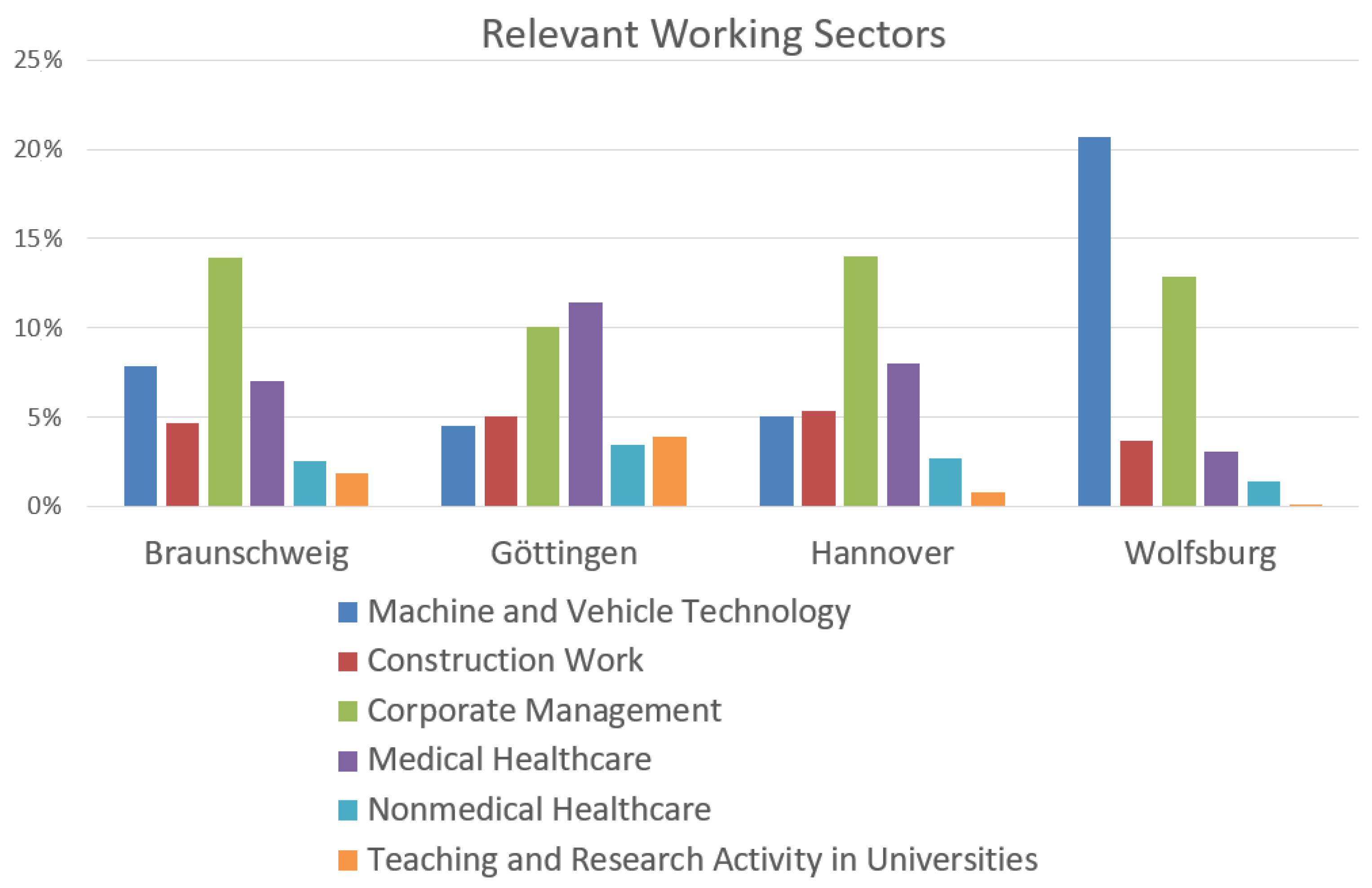
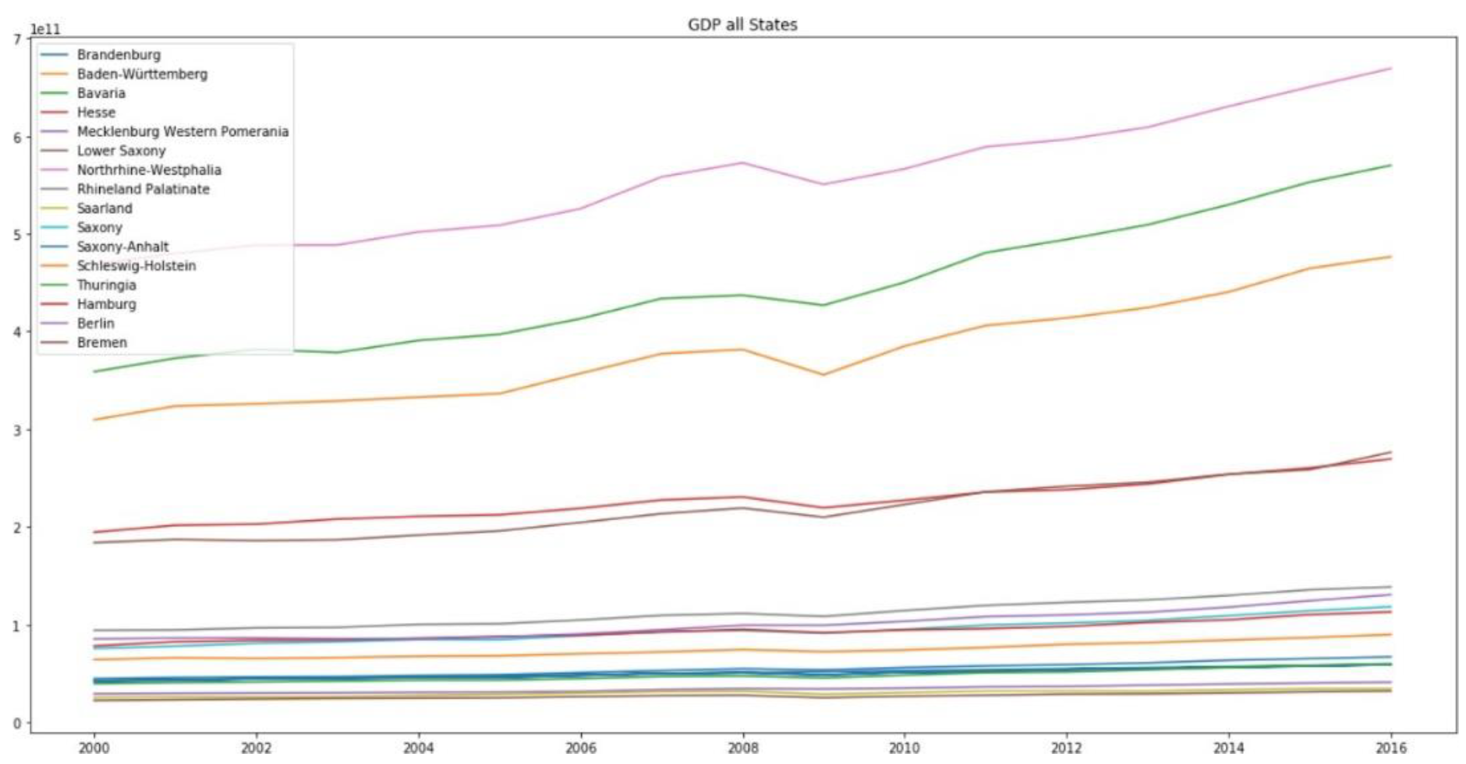
3.1.3. Economic Structure

We scraped GDP data from “GovData” [27] for German cities from 2000 to 2016, including GDP per city, per employee, per resident and per industrial sector. An example of GDP data is shown in Table 7, which leaves out the GDP per industrial sector for simplicity.
Table 8 shows exemplar median incomes for cities and counties with the highest and lowest median income. This shows an income disparity in Germany: after more than two decades of the German reunification [30], the median income of eastern Germany still is 19% lower than in the west; the top ten cities with the highest income are all in western Germany, while all of the five regions with the lowest income are in eastern Germany. Due to the continuous large amounts of workers moving from east Germany to west Germany [31] we conjecture that the median income difference between a large city and its adjacent regions will also influence the commuting behavior, which will be examined in the next section.
For each county/city we obtained data about the median income of employees from the Federal Employment Agency, including the median incomes of men, women and the residents in each region (city/Stadt or county/Landkreis). They are further split into three age groups, ”15 to 25”, ”25 to 55” and ”55 to 65” years old, and three educational levels, ”no professional degree”, ”recognized professional degree” and ”academic degree”. A small example of the data can be seen in Table 9.
The dataset contains the aggregated information of all employees working in each region for the ”place of work” field, including incoming commuters but excluding outgoing commuters; whereas, “place of residence” includes everybody living in the city and excludes incoming commuters. Interestingly, even though it differs on a regional level, on average men are earning 500 € more than women per month. This may be a possible factor to explain the observation in [13], where men are found to be typically more willing to commute than women.
Overall, we can see that the median gross income for the “place of work” is higher than the income for the “place of residence”. This further implies that commuting has a positive impact on income; therefore, it strengthens the conjecture that commuting contributes to the income discrepancy between men and women (https://statistik.arbeitsagentur.de/Statistikdaten/Detail/201712/iiia6/beschaeftigung-sozbe-qheft/qheft-d-0-201712-xls.xls?blob=publicationFile&v=1, accessed on 11 April 2021).

3.1.4. Real Estate Market

We scraped the house and rental prices via the ImmobilienScout24 API [25]. Table 10 shows an example of apartment rental prices.
With the differentiation between cities and counties we have 419 data points. In this example, we include Munich because it indicates the vast difference between the house and apartment prices in Germany.
Since we have only the present housing price data, we add additional data pre-processing to incorporate additional knowledge from other sources and try to reflect the changes over the time as much as possible. For example, we superimpose an increase in housing prices by 21.7% from 2015 to 2018 (this information is from the Federal Statistics Office [32].

3.2. Methods

We use statistical methods to pre-process the data to get an overall view of different potential factors including their dynamic characteristics (where available).
We use linear regression to analyze the influence of factors like housing prices, GDP and median income on commuting decisions, taking housing prices as a specific example.
We use correlation to understand the potential factors related to commuting. To measure the correlation between variables x and y, the Pearson’s correlation coefficient is given by:
r = i = 1 n ( x i x ¯ ) ( y i y ¯ ) i = 1 n   ( x i x ¯ ) 2 i = 1 n   ( y i y ¯ ) 2
where xi and yi are the values of x and y for the ith individual
We use the following machine learning algorithms to predict the commuter number using the identified related features.
  • Linear regression: an easy regression approach used to predict a continuous output (here, commuter number) where there is a linear relationship between the features of the dataset and the output variable. It assumes the input features to be mutually independent.
  • Decision trees: this approach first splits the dataset into smaller subsets and then makes predictions based on what subset a new example would fall into; it re-cursively runs this process until a good match is found. Decision trees make no assumptions on distribution of data and work well with colinearity between input features.
  • Random forest: a random forest aggregates a multitude of decision trees during the training time, each of which independently derives a prediction, then returns the mean prediction (regression) of the individual trees. It is one of the most accurate machine learning algorithms available and works well for many datasets.

4. Results

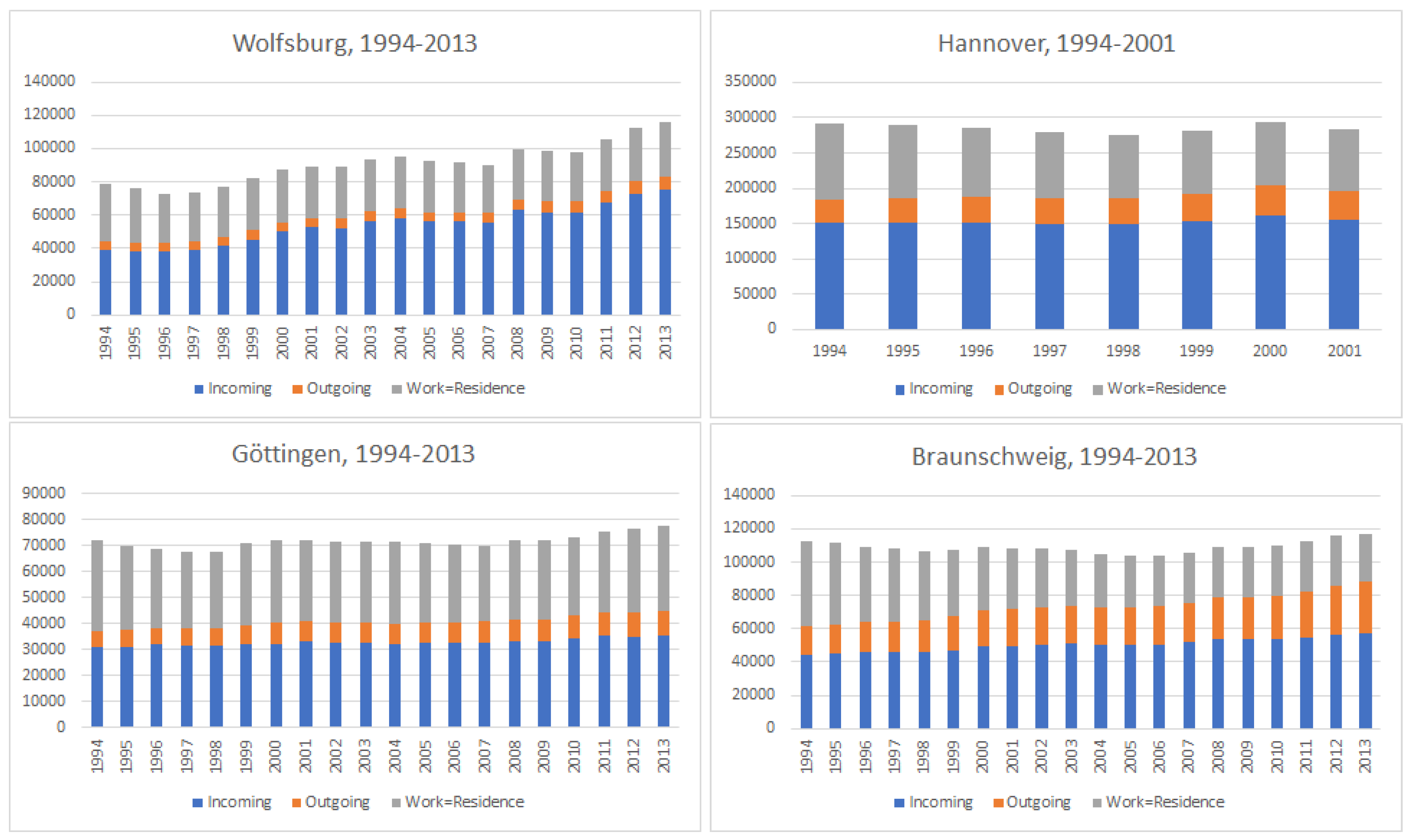
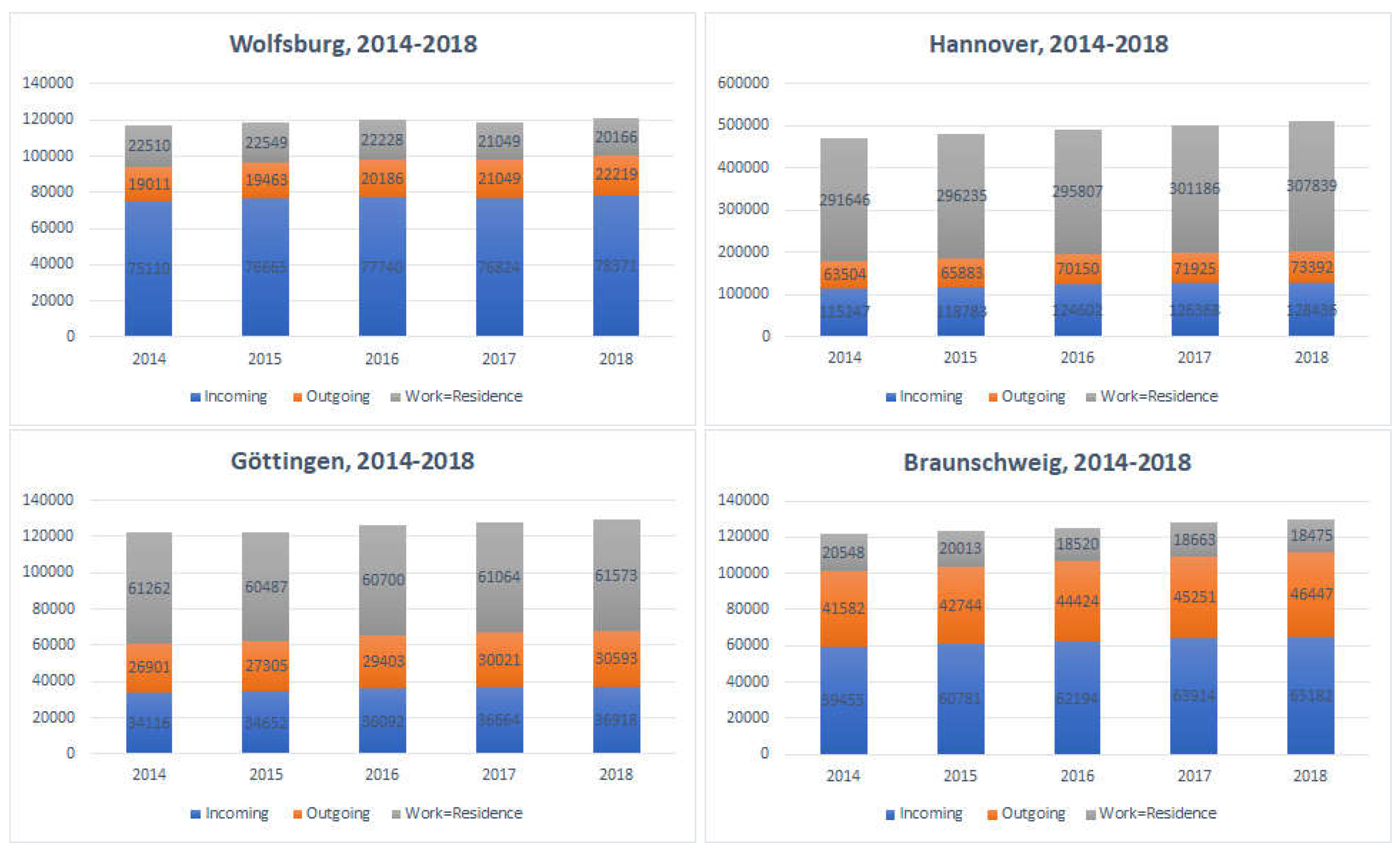
4.1. Commuter Dynamics in Four Exemplar Cities

In the four example cities in State Lower Saxony (Göttingen, Braunschweig, Hannover and Wolfsburg), the number of commuters gradually increases, as shown in Figure 2 for 1994–2013 (except for Hannover which has only data for 1994–2001 and no data for 2002–2013), and Figure 3 for 2014–2018.
The blue line shows the number of incoming commuters, the yellow line shows the number of outgoing commuters and the gray line shows the number of employees living in the same places where they work over the years. We see all commuter numbers increase but there are differences from each other. Wolfsburg denotes the most visible increase, almost doubling its incoming commuters during 1994–2013 due to its increased employment opportunities. Braunschweig and Göttingen’s increases of incoming commuters are more subtle but still easily observable. Hannover, on the other hand, seems to stagnate. As a small university town, Göttingen’s increase in incoming commuters is smaller.
The number of outgoing commuters stays almost the same for Wolfsburg, Hannover and Göttingen. Braunschweig, however, witnesses a big increase. Due to its closeness to Wolfsburg and the massive increase in incoming commuters to Wolfsburg, it is likely due to the strengthened industry in Wolfsburg and that many employees tend to commute there.
Starting from 2014, the Federal Employment Agency provides additional information on how many people live in the same region as they work. It now treats the county of Göttingen as Göttingen instead of the city of Göttingen, as in the 1994–2013 data. This leads to an increase in both incoming and outgoing commuters for Göttingen in 2014.
From the information on “work (place) = residence (place)” in Figure 3, we can see that both Göttingen and Braunschweig have the biggest proportion of their non-commuting employees. Incoming commuters in Braunschweig grew close in number to the non-commuting employees in 2016–2017. Both Wolfsburg (as an industry city) and Hannover (as the state capital) have more incoming commuters than non-commuting employees. Incoming commuters in Wolfsburg are nearly twice the number of non-commuting employees.
To sum up, we can see that the increase of commuters depends heavily on the city’s industry and economic development and the relationship with the adjacent cities.

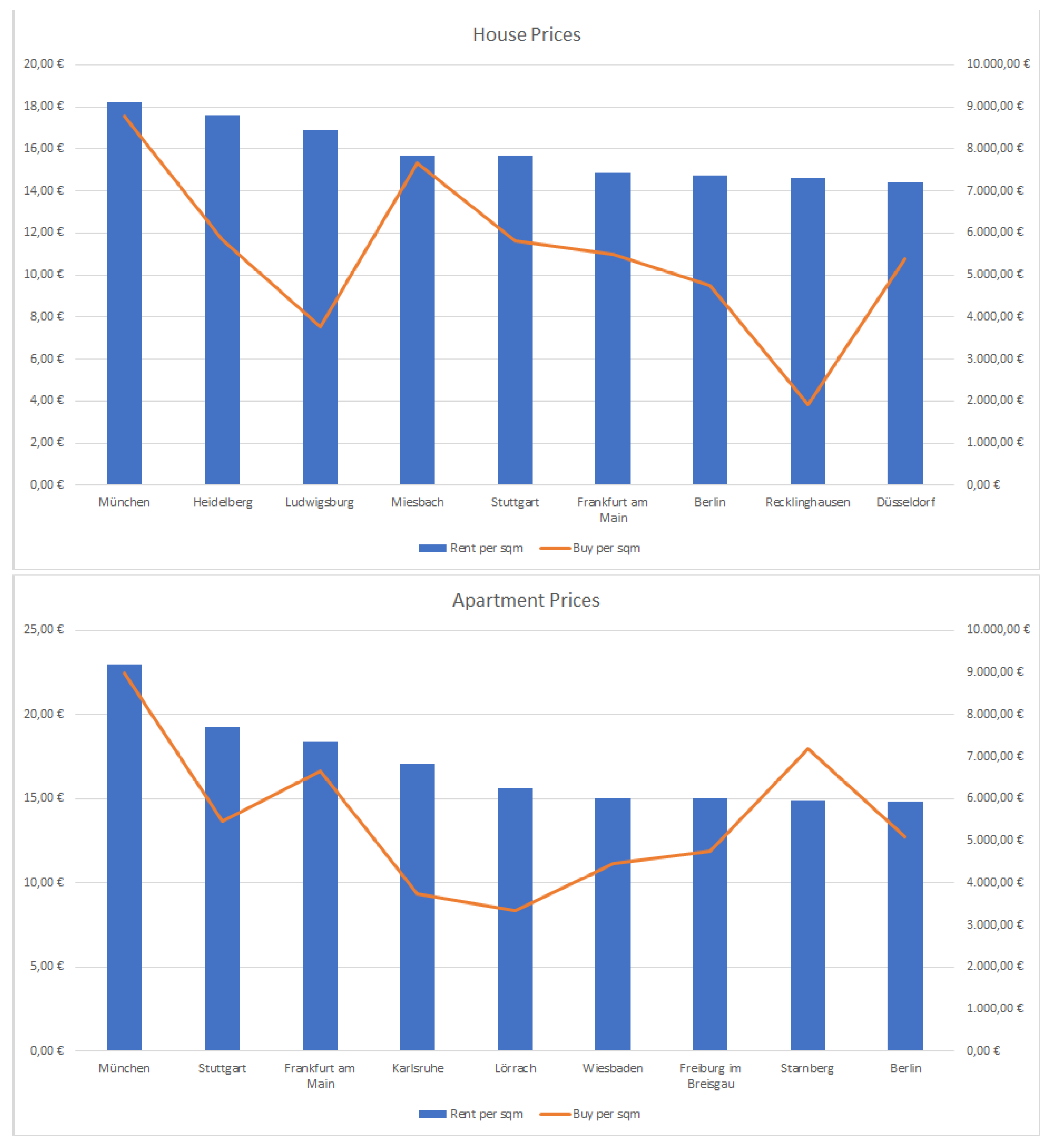
4.2. Housing Prices: Statistics

Housing prices are important for commuting decisions [33,34].
We collected data for over 400 cities in 2019. For most of them, we have house and apartment prices, as well as the rental prices for each type. Furthermore, we have the mean living space and with that can calculate the mean price per sqm. This is the most important part of the data since it allows us to compare the cities based on their living price per sqm.
Housing prices differ greatly for German cities. Many regions in eastern Germany are known for having cheap property, as there are not as many jobs as in western Germany. In the industry sector data from the Federal Employment Agency, we see that there are a total of 150,000 reported jobs, while there are 630,000 reported jobs in western Germany. The regions differ heavily in mean income as well. The median income for western Germany is 2700 e while the eastern Germany median is 2200 e. Therefore, it makes sense that the property prices for eastern Germany are lower than in western Germany. Due to the way Immobilienscout24 returns the data, we could not classify the advertisements to eastern or western Germany. However, if we look at the cheapest property prices, we can verify that most of them are regions in eastern Germany. This can be seen in Table 11.
The five regions with the cheapest apartment rental prices, except for Grafschaft Bentheim which is on the western border to the Netherlands, are in eastern Germany. Apart from some small secluded regions, this trend continues throughout our data.
It is well known that Munich is the most expensive city in Germany [35], followed by Frankfurt and Stuttgart; these three cities are important metropolises for the German industry. In Figure 4, we see the most expensive mean prices per sqm for buying or renting a house or apartment.
The bars indicate the renting price, and the graphs denote the buying price. We see that Munich is the most expensive city to both rent or buy an apartment or a house. It reflects the property market well, having Munich, Stuttgart, Frankfurt, Hamburg, Berlin, Cologne and Mainz in the top 20 most expensive properties in all four categories.

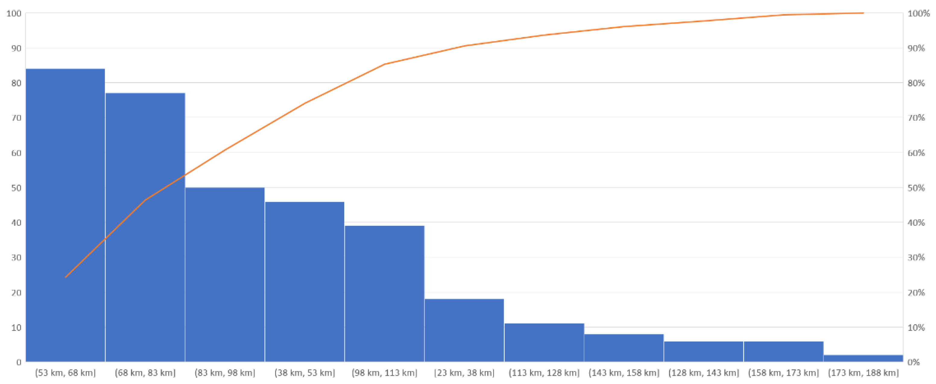
4.3. Commuting Distances: Statistics

Using the calculation method in Section 3.2, the statistical commuting distance data are computed in Table 12.
The average commuting distance of 77 km is from the data on a regional level and therefore does not account for short-haul commuters. The minimal commuting distance is mostly for commuting that is between cities within the same county. Because the Federal Employment Agency lists them as different areas, they have a very short commuting distance with a very high amount of commuters. The maximal value of 183.2 km is for Birkenfeld where many employees are commuting to Bad Kreuznach, which is 140 km away. With both the mean and the median at about 70 km, we can see that these data are balanced and represent the long-distance commuters well. The exact distribution of commuting distances can be seen in Figure 5. The diagram shows the number of cities corresponding to the average commuting distance. The x-axis shows the intervals the cities belong to. These buckets have a size of 15 km each. The y-axis denotes the number of cities that are part of the respective bucket. For example, the column on the far left has 84 cities with an average commuting distance of 53 km to 68 km. The orange line represents the cumulative total, which is almost at 50% after the first two bars. It further shows that most of the commuters are commuting medium distances, between 38 km and 98 km, accounting for 75% of the total data. We can also see that only 10% of the cities have very long or very short distance averages below 38 km, or over 113 km. Our results seem to deviate a bit from Schulze [36] who found that most of the commuters commute up to 25km. The reason is that Schulze used a different data source which can directly compute commuting distances, including for both intra-regional/city and inter-city commuters. With the Federal Employment Agency dataset, we have only aggregated information about inter-city commuters; due to the data provider’s privacy restrictions we had to calculate the commuting distance ourselves.
Overall, the commuter data are not very balanced with many small regions with few commuters, and a smaller amount of big cities with very many commuters. Additionally, the type of city plays a key role in the observable commuting patterns. With our regional data, we are able to validate the findings of previous studies, e.g., by confirming that male commuters outnumber female commuters.

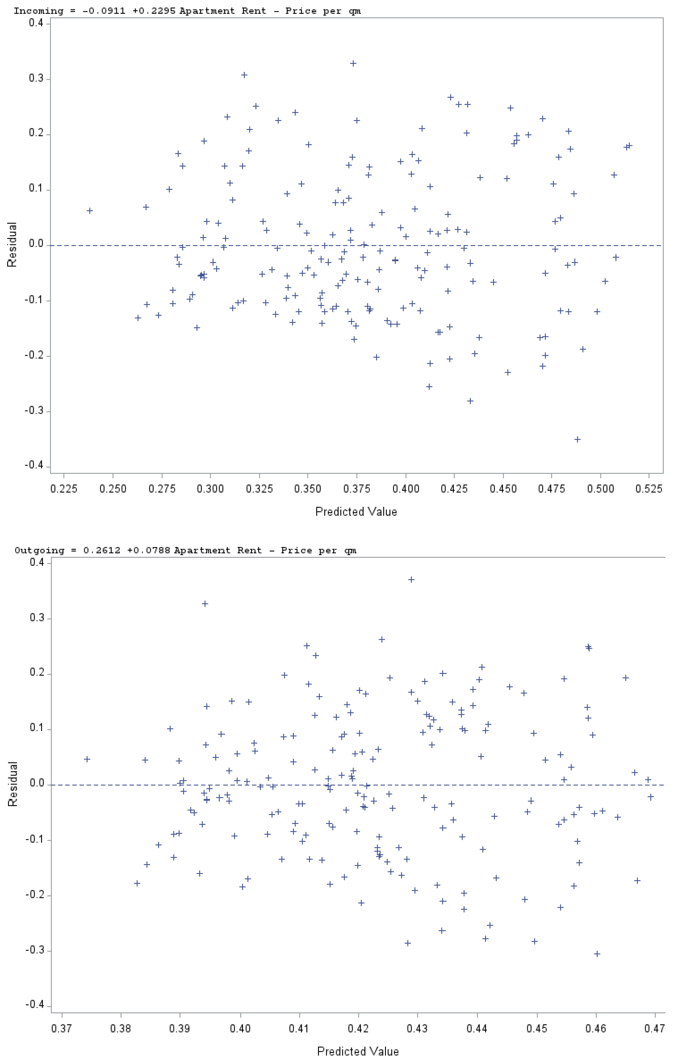
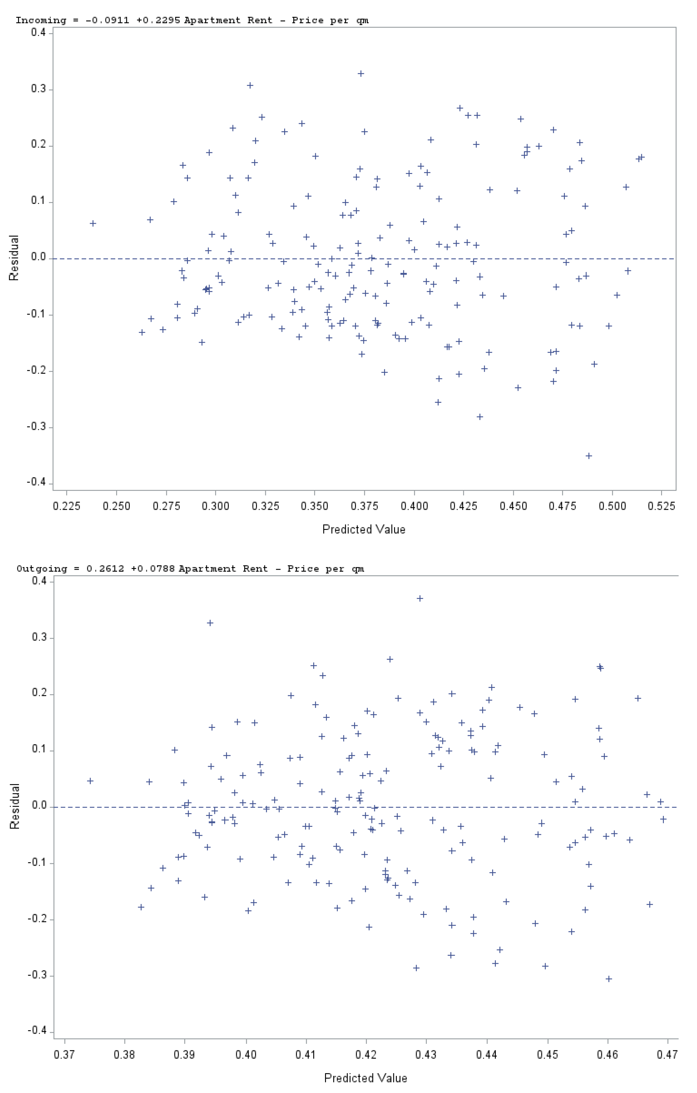
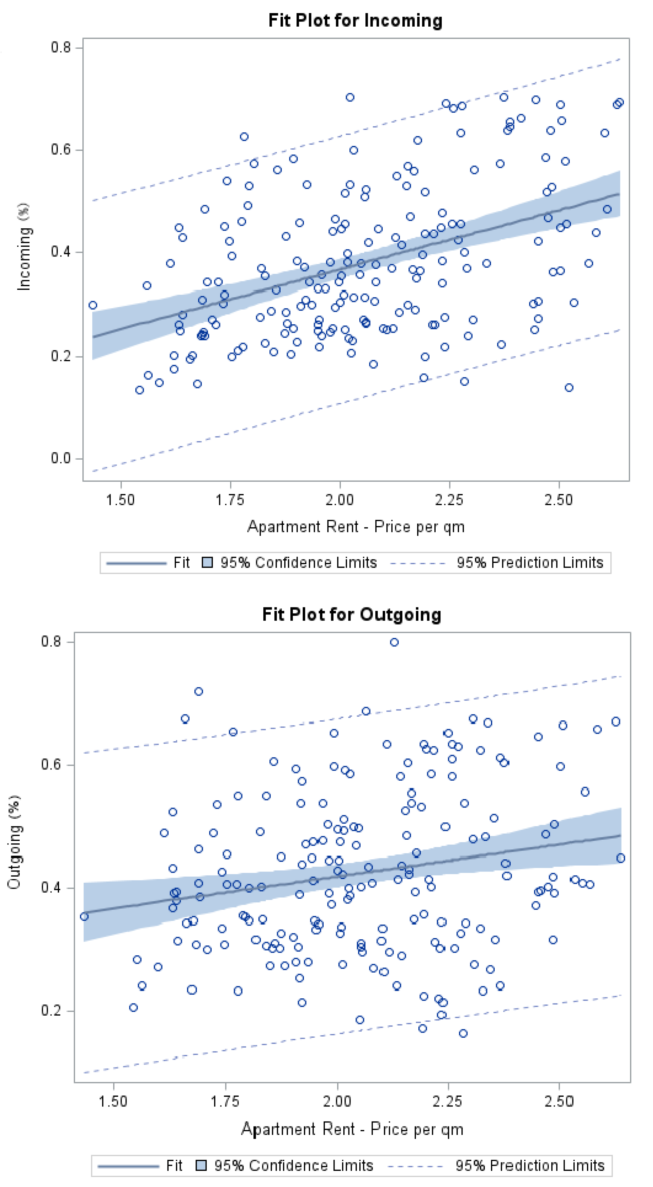
4.4. Housing Prices vs. Commuters: Linear Regression Results

We investigate the influence of the housing prices in regards to the number of commuters. To illustrate this, we conduct regression studies on apartment rental prices vs. the ratios of incoming and outgoing commuters to the number of local employees. The cases of other prices (apartment buying prices, house rental prices, house buying prices) are similar and skipped here due to space limit.
Two simple ordinary least squares (OLS) linear regression models are built for analyzing the relationship between apartment rental price (€ per sqm) and the ratio of commuters (against the local employees). The fit plots are shown in Figure 6. Both models suffer from heteroscedasticity which we can detect from both White’s test results (Table 13, p-value <0.05) and residual plots as shown in Figure 7. To fix the heteroscedasticity, we apply the heteroscedasticity-consistent covariance matrix estimator [33].
Using OLS linear regression for the log transformation of the apartment rental price (e per sqm), the result parameters are shown in Table 14; further model diagnosis reveals that the models’ parameters are significant and there is no heteroscedasticity inside anymore (p-Value >0.05).
We can see the relationship between the number of commuters and the logged unit price to rent an apartment in Figure 8. Both figures show an increasing trend, indicating a higher average number of corresponding commuters for a higher rental price. Further- more, the number of incoming commuters increases faster with a higher rent cost than the number of outgoing commuters. The number of outgoing commuters also increases, likely due to being in bigger cities with more inhabitants.
Again, we see that the incoming commuters increase quickly for higher apartment prices; the deviation is high for higher apartment prices due to the distribution of the data. Therefore, we rely on medium house prices and medium apartment prices.
Overall, the more expensive the real estate, the more employees will commute over long distances. This is in accordance with Boje et al. [34] who stated that according to location theory, rationally acting individuals compare the resulting benefit with the costs of commuting. If the costs outweigh the benefits, as they would have to pay a high percentage of his or her income for rent, they would give up renting in the workplace city and consider commuting instead. This behavior can be observed in our data, e.g., fewer employees in cities with low housing prices will decide to commute than in cities with higher housing prices.

4.5. Housing Prices and Income

We also analyze the relationship between housing prices and the median income. Similar to the previous subsection, our first results also show heteroscedasticity but can be fixed by the heteroscedasticity-consistent covariance matrix estimator; the results are omitted here again for the space limit, which explains that with an increasing median income, the apartment rent rises as well.
The result is expected, as it is logical that the real estate market and the median income are related to each other. Nonetheless, as the income has a strong link to the apartment and housing prices, it indicates a link to the commuter data as well.

4.6. GDP and Median Income

In this subsection we will take a closer look at our median income and GDP data.
While the individual city-level GDP data depict well the productivity of the city, the aggregated GDP information on the state level (Figure 9) shows a clear trend in the German economy distribution.
As shown in Figure 9, North Rhine-Westphalia has the highest GDP, followed by Bavaria and Baden-Württemberg. North Rhine-Westphalia is well known for the Ruhrgebiet, which is a composite of industrial cities and thus a big metropolitan area. Bavaria also has important cities for the German industry like Nuremberg and Munich. Hamburg and Berlin are in the 4th and 5th place, respectively. This is no surprise, as these two cities are the biggest in Germany and hence have a great influence on the German economy. Overall, we see that the states in west Germany have higher GDP than their counterparts in east Germany.

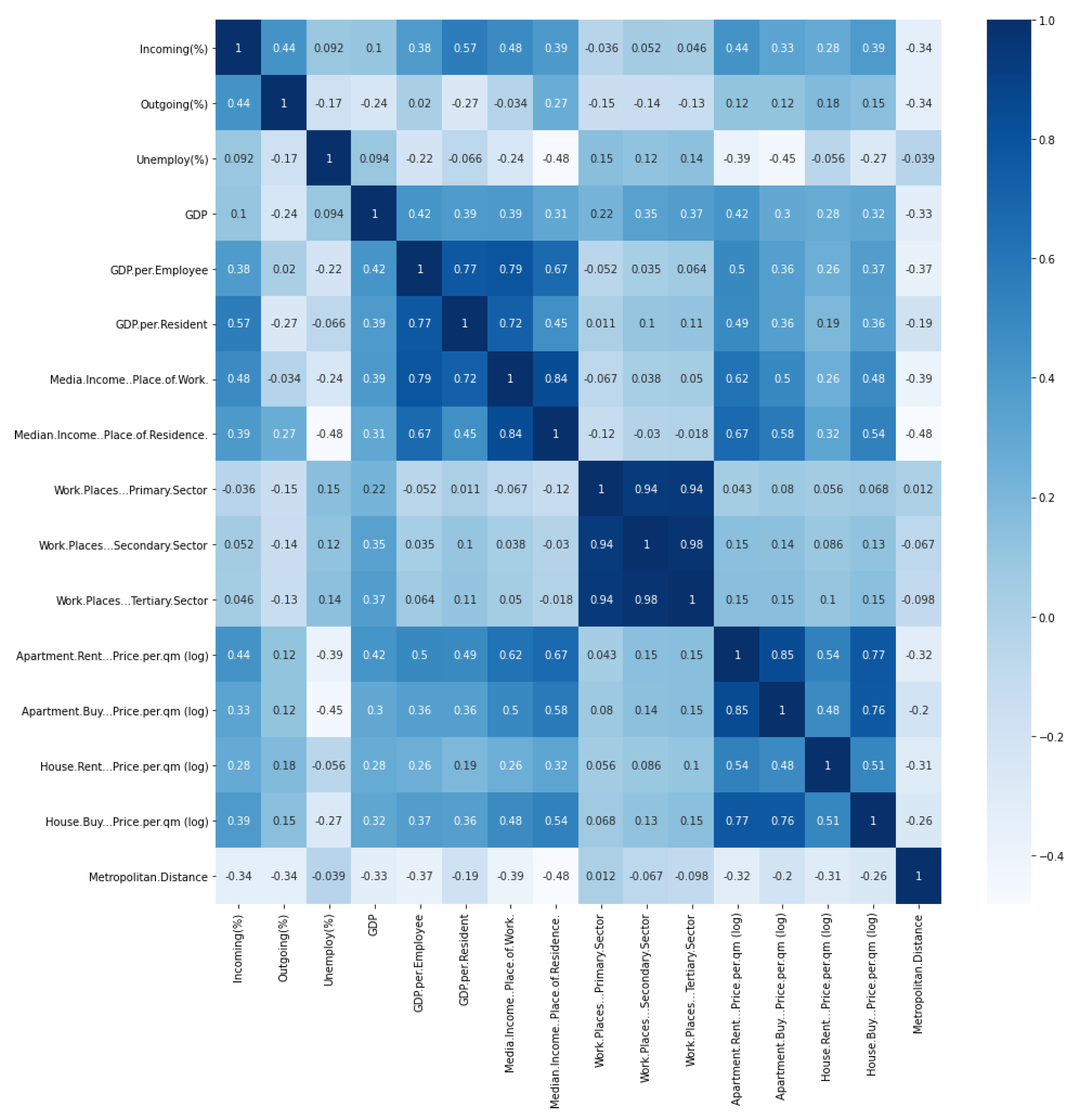
4.7. Correlation Results

After analyzing all the data separately, we study their correlation with each other with a focus on the correlation with the commuting data.
To understand the most important reason behind commuting, we limit the correlation matrix to the 16 most important factors (see Table 2). The result is shown in Figure 10.
Beyond the highest correlations between the jobs in any two of the three industrial sectors, primary sector, secondary sector and tertiary sector, another high correlation is found between incoming commuters and outgoing commuters (in percentage of local employees). Except for commuting-related factors, the highest negative correlation is found between median income and metropolitan distance.
Now we examine the factors behind commuting based on this correlation matrix:
  • The matrix shows that the most important factor behind commuting is the GDP per resident of the city, as among all factors it has the highest Pearson’s correlation coefficient with incoming commuters in percentage of the local employers (0.57) and the lowest (and negative) coefficient with outgoing commuters in percentage of the local employers (−0.22). This is somewhat surprising, as we expected that the median income and housing prices may have a more important influence on commuting decisions.
  • The median incomes of work and living places are also important. The median income in the place of work is highly influential on incoming commuters, as more employees may commute if they receive a higher income. How much they earn in their residence is influential to both commuting groups. The income in the place of residence is a main factor of commuting, either leaving the city or coming there, because if it is high, many people will decide to commute there; if it is low, more people will leave the region to work somewhere else.
  • The third most important factor for incoming commuters is the apartment price; more expensive apartments seem to be a factor related to employees commuting. A plausible reason behind this relation is that if the cost–benefit ratio of buying an apartment is bad, the employees may consider commuting over longer distances. For outgoing commuters, the distance to the next metropolitan area is very important. This means that if the distance to the next metropolitan area increases, employees are less likely to leave their region to commute, given the cost–benefit ratio of long-haul commuting.
  • An interesting anti-correlation can be found between the outgoing commuters and the metropolitan distance. If the metropolitan distance increases, the outgoing commuters decrease, as their commuting distance would get longer and become most likely unprofitable.
  • A surprising high correlation can be found between commuters and the unemployment data. This has a big influence on both incoming and outgoing commuters. This may be related to the fact that most bigger cities tend to have a higher unemployment rate.
  • In regard to jobs (workplaces), the secondary and tertiary sectors are more influential on commuters than primary sectors, likely due to their high number of employees. For example, there were 82.3% jobs in the tertiary sector, and 17.2% in the secondary sector, in contrast to 0.5% in the primary sector as of 2017 [32]. Workplaces in the primary sector even show an anti-correlation with commuters, indicating that most farmers tend to not commute.

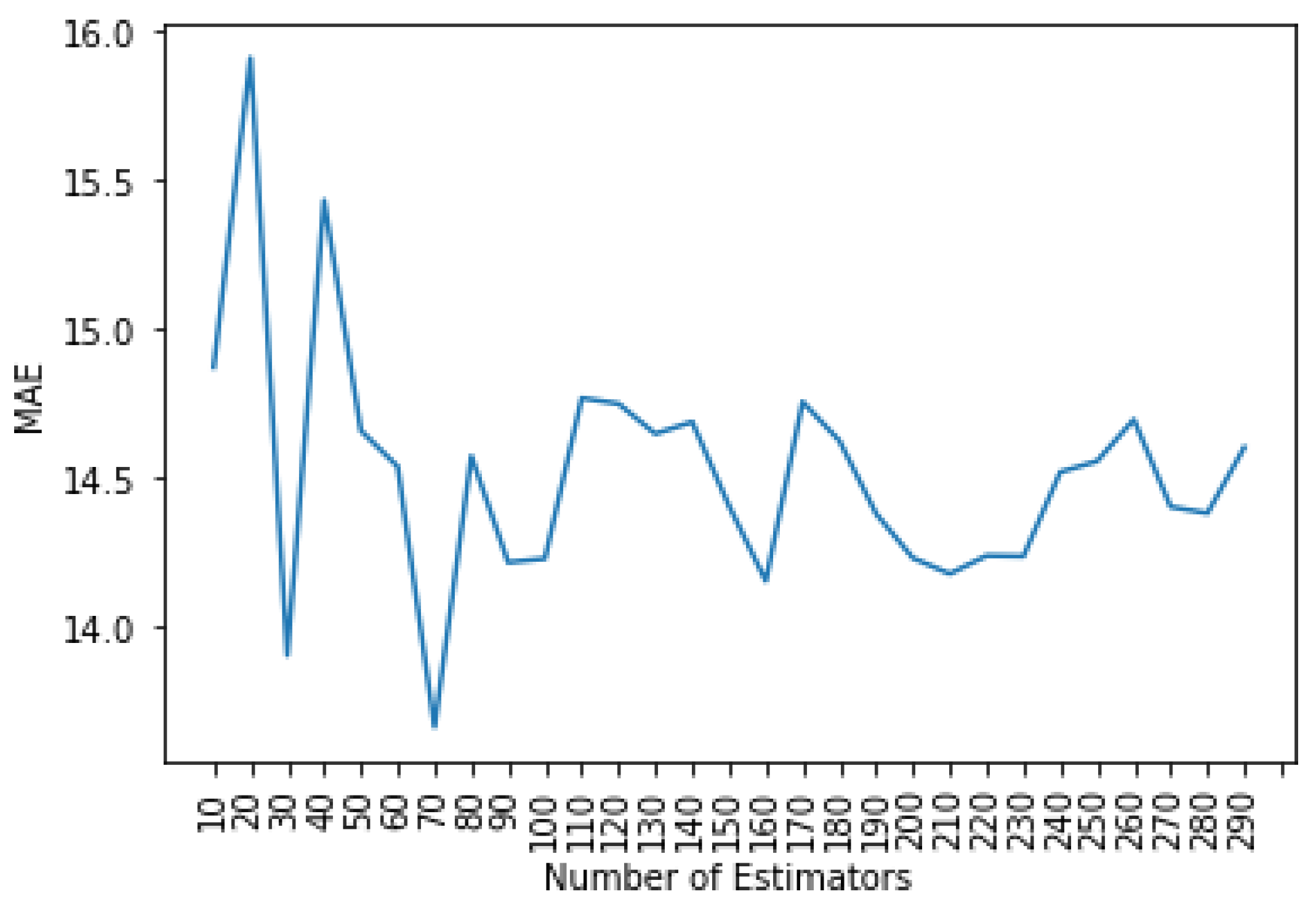
4.8. Commuter Prediction Results

As commuting is an important part of social life, for city and infrastructure planners, it is helpful to predict the commuting trend for the next years. Since the data collection of the Federal Employment Agency changed in 2013, we mainly focus on predictions using data from 1994 to 2012 to predict the number of commuters in 2013 for each city.
First, we generate our time series data using the TimeSeriesSplit function of scikit-learn, which splits the commuter data into different time frames. We then train a linear regression model (with heteroscedasticity detection and correction procedures), a decision tree model and a random forest model (with 100 decision trees as baseline), respectively, to predict the incoming and outgoing commuters for each city in 2013.
Three metrics of measuring the prediction accuracy are used here: (1) The mean absolute error (MAE) means that we are on average off by a certain number of commuters. (2) The mean squared error (MSE) measures the average of the squares of the errors; the closer to zero the MSE is, the better. (3) The root mean squared error (RMSE) is the root of the MSE and measures the accuracy of a forecast; again, the closer to zero the better, where a value of zero would mean that the prediction is perfect. The results for accuracies for incoming commuters and outgoing commuters in 2013 using the 1994–2012 data are shown in Table 15. The following observations can be made:
In general, linear regression yields the worst performance as the input features do not hold collinearity; meanwhile, decision trees achieve much reduced MAE, MSE and RMSE. Random forest provides further improvements on prediction accuracy. An outlier is the MSE and RMSE are better for predicting outgoing commuters using linear regression compared to using decision tree or random forest algorithms, which may be attributed to the limited features available for the better balanced outgoing commuter data; more concrete reasons have to be found out.
Overall accuracy is reasonably good, considering the mean and median (50%-percentile) commuters numbers (see Table 3) of incoming commuters (2820 and 232) against its MAE (14.36 in the case of random forest, 18.38 for decision tree), and outgoing commuters (3010 and 651) against its MAE (41.97 for random forest, 44.58 for decision tree). This reflects only roughly 0.5–6.8% of absolute errors on average in the prediction.
The prediction accuracy for incoming commuters is generally better than that of outgoing commuters. This is affected by the highly unbalanced commuter data that the small numbers of incoming commuters in the cities are much more heavily distributed than large numbers, compared to outgoing commuters (see Table 3). When the overall incoming commuting number for a city is small, it is easier to predict with lower MAE than to predict the larger number.
We then examine how the number of decision trees affects the prediction accuracy. We try it at low as 10 and as high as 300 decision trees. The corresponding MAE can be seen in Figure 11.
We see that the MAE fluctuates between 14.2 and 14.7 after 90 estimators. Hence, it does not make much sense to increase the number of trees over 100. The low MAE at 70 estimators is most likely due to the randomness of the trees.
The important feature of the decision trees (see Table 16) shows that the last two (i.e., year 2011 and year 2012) and the four to last year (i.e., year 2009) are the most important ones.
This result is expected, as we are working with a time series and the number of commuters of the next year is mostly influenced by the most recent data.

5. Discussion

Although this work focuses on the Germany case, we believe the methodology proposed in this paper can be extended for studying commuting behaviors in other countries, as most countries have published their per-city level employment, income, GDP and commuter information online, and there are abundant other sources like LinkedIn and Facebook as well as real estate market websites to gain access to further information.
Furthermore, it may be useful to include the total number of residents (rather than just socially insured employees) in the analysis, which covers the whole commuter population such as students, who may contribute to the peak hour congestion. Furthermore, more studies on commuting distances may be also useful to understand the commuting behavior from cost–benefit tradeoffs.
Additionally, the social, educational and medical facilities could be considered as potential additional factors. Including data like the number of hospitals, doctors or kindergartens, or even green areas and points of interest may be helpful for better under- standing commuter decisions and for the prediction of commuters. Furthermore, with the increase in housing prices over the last years, we think that it could be interesting to perform an in-depth analysis of the connection between the real estate market and commuters. We only had the house price data for one year, so looking at other historic data sources may reveal new information.
Our commuter prediction is currently only based on our time-series commuter data during 1994–2013, which can be extended for later (2014–2018) data which contain richer information such as housing prices, GDP and jobs in different sectors in each county or city. The results are still yet to be improved by future fine-tuning of the models and feature engineering, and subject to further analysis on how individual factors affect the performance of commuter predictability. Nonetheless, our initial results show that even with simple methods a reasonably good prediction can be achieved. This will bring value as it helps the city and infrastructure planners to better understand the commuting trend and deploy better countermeasures, e.g., for clogged roads or traffic jams in a short term, or developing alternative mobility options other than cars in a longer term.
Lastly, the current COVID-19 pandemic may significantly change commuting behavior. This may open a large body of new insights for future exploitation.

6. Conclusions

The question of what leads to commuting is a critical issue for modern society’s development. Most prior studies focused on a small set of factors constrained by limited scale in terms of timespans, space and commuter numbers. To fill this gap, in this paper, we explored a big data approach, by collecting data from multiple publicly accessible sources and performing a systematic analysis on the potential influencing factors from four perspectives (the cities’ economic structure, labor and real estate markets as well as commuting patterns). We found that the GDP, the median income and the price of buying or renting an apartment or a house in potential places for work and residence, as well as their distance to the next metropolitan area, are key factors in the decision to commute. We showed these main driving factors behind commuting in our data, confirming some findings in previous work and offering some new insights such as GDP, detailed categories of housing prices and job market in different sectors with the aid of much richer data sources. We hope that such a data-driven approach will open this field of study to more coverage in the future, as commuting is an important part of daily life in Germany (and worldwide).
Additionally, we leveraged several machine learning models to predict the number of commuters. Our results show it is possible to forecast the commuters quite precisely.

Author Contributions

Conceptualization, H.C. and X.F.; methodology, X.F. and H.C.; data collection and processing, S.V.; writing—original draft preparation, S.V. and H.C.; writing—review and editing, H.C. and X.F.; data curation, X.F.; supervision, H.C. and X.F. All authors have read and agreed to the published version of the manuscript.

Funding

This research was funded by the Fundamental Research Funds for the Central Universities (Grant No. 2020JJ014, YY19SSK05), and the European Union’s Horizon 2020 research and innovation program under the Marie Sklodowska-Curie grant agreement No. 824019.

Institutional Review Board Statement

Not applicable.

Informed Consent Statement

Not applicable.

Data Availability Statement

All datasets related to this paper can be obtained in the URLs specified in references [7,25,26,27,32].

Conflicts of Interest

The authors declare no conflict of interest.

References

  1. Hamedmoghadam, H.; Jalili, M.; Vu, H.L.; Stone, L. Percolation of heterogeneous flows uncovers the bottlenecks of infrastructure networks. Nat. Commun. 2021, 12, 1254. [Google Scholar] [CrossRef]
  2. DGB. Mobilität in der Arbeitswelt: Immer Mehr Pendler, Immer Größere Distanzen. Arb. Aktuell. 2016. Available online: https://www.dgb.de/themen/++co++2dee53d6-d19c-11e5-9018-52540023ef1a (accessed on 11 April 2021).
  3. Borck, R.; Wrede, M. Subsidies for intracity and intercity commuting. J. Urban. Econ. 2009, 66, 25–32. [Google Scholar] [CrossRef] [Green Version]
  4. Lee, C. Metropolitan sprawl measurement and its impacts on commuting trips and road emissions. Transp. Res. Part. D Transp. Environ. 2020, 82, 102329. [Google Scholar] [CrossRef]
  5. Takayama, Y.; Ikeda, K.; Thisse, J.-F. Stability and sustainability of urban systems under commuting and transportation costs. Reg. Sci. Urban. Econ. 2020, 84, 103553. [Google Scholar] [CrossRef]
  6. Pendeln in Deutschland: 68% nutzen Auto für Arbeitsweg. Available online: https://www.destatis.de/DE/Themen/Arbeit/Arbeitsmarkt/Erwerbstaetigkeit/Tabellen/pendler1.html?nn=206552/ (accessed on 11 April 2021).
  7. Bundesagentur für Arbeit. Available online: https://statistik.arbeitsagentur.de/ (accessed on 11 April 2021).
  8. Dargay, J.M.; Clark, J. The determinants of long-distance travel in Great Britain. Transp. Res. Part. A 2012, 46, 576–587. [Google Scholar] [CrossRef]
  9. Kalter, F. Pendeln statt Migration? Z. Soziologie 1994, 23, 460–476. [Google Scholar] [CrossRef] [Green Version]
  10. Ding, N.; Bagchi-Sen, S. An Analysis of Commuting Distance and Job Accessibility for Residents in a U.S. Legacy City. Ann. Am. Assoc. Geogr. 2019, 109, 1560–1582. [Google Scholar] [CrossRef]
  11. Dauth, W.; Haller, P. Is there loss aversion in the trade-off between wages and commuting distances? Reg. Sci. Urban. Econ. 2020, 83, 103527. [Google Scholar] [CrossRef]
  12. Clark, W.A.V.; Burt, J.E. The impact of workplace on residential relocation. Ann. Assoc. Am. Geogr. 1980, 70, 59–66. [Google Scholar] [CrossRef]
  13. Eckey, H.-F.; Kosfeld, R.; Türck, M. Pendelbereitschaft von Arbeitnehmern in Deutschland. Raumforsch. Raumordn. 2007, 65, 5–14. [Google Scholar] [CrossRef]
  14. Haas, A.; Hamann, S.; Pendeln—Ein zunehmender Trend, vor allem bei Hochqualifizierten: Ost-West-vergleich. IAB-Kurzbericht. 2008. Available online: http://hdl.handle.net/10419/158268 (accessed on 31 March 2021).
  15. Andersson, M.; Lavesson, N.; Niedomysl, T. Rural to urban long-distance commuting in Sweden: Trends, characteristics and pathways. J. Rural. Stud. 2018, 59, 67–77. [Google Scholar] [CrossRef]
  16. Simpson, W. Workplace Location, Residential Location, and Urban Commuting. Urban. Stud. 1987, 24, 119–128. [Google Scholar] [CrossRef]
  17. Levinson, D.M. Job and housing tenure and the journey to work. Ann. Reg. Sci. 1997, 31, 451–471. [Google Scholar] [CrossRef] [Green Version]
  18. Levinson, D.M. Accessibility and the journey to work. J. Transp. Geogr. 1998, 6, 11–21. [Google Scholar] [CrossRef] [Green Version]
  19. Huinink, J.; Feldhaus, M. Fertilität und Pendelmobilität in Deutschland. Z. Bevölkerungswissenschaft 2012, 37, 463–490. [Google Scholar]
  20. Chidambaram, B.; Scheiner, J. Understanding relative commuting within dual-earner couples in Germany. Transp. Res. Part. A Policy Pr. 2020, 134, 113–129. [Google Scholar] [CrossRef]
  21. Reuschke, R. Job-induced commuting between two residences—characteristics of a multilocational living arrangement in the late modernity. Comp. Popul. Stud. 2010, 35, 107–134. [Google Scholar]
  22. Mitra, S.K.; Saphores, J.-D.M. Why do they live so far from work? Determinants of long-distance commuting in California. J. Transp. Geogr. 2019, 80, 102489. [Google Scholar] [CrossRef]
  23. Clark, W.A.; Huang, Y.; Withers, S. Does commuting distance matter? Commuting tolerance and residential change. Reg. Sci. Urban. Econ. 2003, 33, 199–221. [Google Scholar] [CrossRef]
  24. Dickerson, A.; Hole, A.R.; Munford, L.A. The relationship between well-being and commuting revisited: Does the choice of methodology matter? Reg. Sci. Urban. Econ. 2014, 49, 321–329. [Google Scholar] [CrossRef]
  25. Immobilienscout24 API. Available online: https://api.immobilienscout24.de/ (accessed on 11 April 2021).
  26. Google Maps API. Available online: https://developers.google.com/maps/documentation/?hl=de (accessed on 11 April 2021).
  27. Govdata. Available online: https://www.govdata.de (accessed on 11 April 2021).
  28. Sermons, M.; Koppelman, F.S. Representing the differences between female and male commute behavior in residential location choice models. J. Transp. Geogr. 2001, 9, 101–110. [Google Scholar] [CrossRef]
  29. White, M.J. Sex differences in urban commuting patterns. Am. Econ. Rev. 1986, 76, 368–372. [Google Scholar]
  30. Geib, T.; Lechner, M.; Pfeiffer, F.; Salomon, S.; Die Struktur der Einkommensunterschiede in Ost-und Westdeutschland ein Jahr nach der Vereinigung. ZEW Discuss. Pap. 1992. Available online: http://hdl.handle.net/10419/29430 (accessed on 31 March 2021).
  31. Fendel, T. Migration and Regional Wage Disparities in Germany. Jahrbücher Natl. Stat. 2016, 236, 3–35. [Google Scholar] [CrossRef]
  32. Federal Statistics Office (Statistisches Bundesamt). Available online: https://www-genesis.destatis.de/ (accessed on 11 April 2021).
  33. MacKinnon, J.G.; White, H. Some Heteroskedasticity Consistent Covariance Matrix Estimators with Improved Finite Sample Properties. J. Econom. 1985, 29, 305–325. [Google Scholar] [CrossRef] [Green Version]
  34. Boje, A.; Ott, I.; Stiller, S.; Entwicklungsperspektiven für die Stadt Hamburg: Migration, Pendeln und Spezialisierung. HWWI Policy Pap. 2010. Available online: https://econpapers.repec.org/RePEc:zbw:hwwipp:124 (accessed on 31 March 2021).
  35. Kholodilin, K.A.; Mense, A. Wohnungspreise und Mieten steigen 2013 in vielen deutschen Großstädten weiter. DIW Wochenber. 2012, 79, 3–13. [Google Scholar]
  36. Schulze, S.; Einige Beobachtungen zum Pendlerverhalten in Deutschland. HWWI Policy Pap. 2009. Available online: https://econpapers.repec.org/RePEc:zbw:hwwipp:119 (accessed on 31 March 2021).
Figure 1. Industry Sectors for Example Cities (Source: Federal Employment Agency).
Sustainability 13 06320 g001
Figure 2. Number of Commuters from 1994 to 2013 (Source: Federal Employment Agency).
Sustainability 13 06320 g002
Figure 3. Number of Commuters from 2014 to 2018 (Based on Source: Federal Employment Agency).
Sustainability 13 06320 g003
Figure 4. Highest House and Apartment Prices (EURO/sqm) (Source: ImmobilienScout24).
Sustainability 13 06320 g004
Figure 5. Pareto Chart of Commuter Distance.
Sustainability 13 06320 g005
Figure 6. Apartment Rental Prices (€ per sqm) vs. Commuters (%).
Sustainability 13 06320 g006
Figure 7. Apartment Rental Prices (€ per sqm) vs. Number of Commuters: Residuals.
Sustainability 13 06320 g007
Figure 8. Logged Values of Apartment Rental Prices (e per sqm) vs. Commuters (%).
Sustainability 13 06320 g008
Figure 9. GDP of German States (2017).
Sustainability 13 06320 g009
Figure 10. Correlation Matrix.
Sustainability 13 06320 g010
Figure 11. MAE in Relation to the Number of Estimators.
Sustainability 13 06320 g011
Table 1. Datasets, Methods and Factors Considered in Previous Literatures.
LiteratureMaterial (Data)MethodFactors Considered
Clark [12]556 residential relocations in Milwaukee metropolitan area, USA (1962–1963)Probability model & testsShort-haul commutes, workplace’s attraction, relocation willingness
Simpson [16] Household transportation survey data in Greater London, UK (1971–1972) and Metropolitan Toronto Travel survey data of 3508 households in Toronto, Canada (1979)RegressionCommuting distance, job opportunity, skilled or not, family status, age, job changed or not
Kalter [9]The “Socio-Economic Panel (SOEP)–West” data of Germany in 1985Explanatory modelCosts of commuting and migration, real estate and labor markets
Levinson [18]Travel survey data of 8000 households in Montgomery County, Washington DC, USA in 1991RegressionFamily status, housing type, age, gender, income, sector, employer’s attitude on home office, location within the city, commuting time
Clark et al. [23]Survey data of 2000 households in greater Seattle area in USA (1989–1990, 1992–1994 and 1996–1997)Probability modelCommuting distance, residential location, work-place location, computing time
Eckey et al. [13]Data of 142,129 commuters in Germany (2003–2005)A traffic prognosis program VISUMCommuting distance, commuting time, gender, professional types (white vs. blue-collar), housing supply, income
Haas & Hamann [14]Two datasets about German commuters in 1995–2005Basic comparisonEducational levels, commuting distance, region is east or west Germany, employment situation
Reuschke [21]2007 questionnaires on 4 metropolises in Germany (Munich, Stuttgart, Düsseldorf, Berlin) in spring 2006, plus telephone interview on 20 commuters in spring 2009Logistic regressionFamily status and living situations, number of residential locations
Dargay & Clark [8]Survey data from National Travel Surveys (NTSs) of UK in 1995–2006Econometric modelsGender, age, employment status, household composition, commuting distance
Huinink et al. [19]Survey data from Family Panel of Germany in 2008–2009Regression, panel modelFertility behavior, gender, employment status, education, partnership status, intention of having and the number of children
Dickerson et al. [24]Survey on 16,000 individuals in UK in 1996–2008Linear fixed-effects (FE)modelCommuting time, transport mode, age, hours worked, household income, marital status, children number, university degree or not
Andersson et al. [15]Micro data for all inhabitants in Sweden spanning two decadesLogit modelCommuting distance, workplace/residence changed or not, income, age, gender, highest degree, family status, sector, occupation type
Mitra & Saphores [22]Survey data of 18,012 households in California, USA in 2012A generalized
structural equation model
Socio-economic variables, vehicle ownership, land use, and housing costs
Ding & Bagchi-Sen [10]Longitudinal Employer–Household Dynamics (LEHD) data set of Buffalo, New York in 2014RegressionIncome, age, sector
Dauth &Haller [11]Dataset on the employment biographies of German workers with geo-coordinates places of residence and
work of Germany in 2000–2014
Statistics, correlation analysisIncome, place of residence, place of work, employment status of each worker
Chidambara & Scheiner [20]Survey data of 4775 households in Germany in August 2012–July 2013Regression analysisEconomic power, car access, labor and domestic work-sharing and preferences on work-sharing
Table 2. Potential Factors Influencing Commuting Decisions.
Labor MarketEconomic StructureReal Estate MarketCommuting Patterns
Jobs (primary sector)
Jobs (secondary sector)
Jobs (tertiary sector) Unemployed
GDP
GDP per worker
GDP per resident
Median income (place of work)
Median income (place of residence)
Apartment rent price
Apartment buy price
House rent price
House buy price
Incoming commuters
Outgoing commuters Commuting distance
Table 3. Commuters on a Municipality Level 2017 (Source: Federal Employment Agency).
IncomingOutgoingForeignersGermansFemaleMale<2020–25≥55noCommutingBusiness
Count11,38511,38511,38511,38511,38511,38511,38511,38511,38511,38511,385
Mean28203010952835243155015218713118156315630
Std16,19112,94413,973101,29252,70561,9422729917621,618104,6447719
Min00000000000
25%432345212110138715571513
50%2326512470834340623541557842
75%1139190114022411111130070182496452150
Max411,672423,964694,0525,993,8725,997,8723,614,232175,175538,6841,268,7056,283,373434,147
Table 4. Incoming and Outgoing Commuters for the Four Example Cities. (Source: Federal Employment Agency. Except For This Column, All Other Data Are Meant for 2017. * The Data for Göttingen After 2013 Were Based on the Whole County of Göttingen; the Municipality Göttingen Alone had 120,000 Residents in 2017).
CityResidences 1994 ResidentsIncomingOutgoingIncoming %Outgoing %
Braunschweig256,000250,00065,00035,00026%14%
Göttingen128,000330,000 *90,000 *250,000 *27% *8% *
Hannover526,000540,000180,000600,00033%11%
Wolfsburg124,000125,00080,000100,00064%8%
Table 5. Incoming and Outgoing Commuters, County-Level, 2017 (Source: Federal Employment Agency).
(a) Incoming Commuters, 2017
TotalMaleFemaleGermansForeigners
Count79,80379,80379,80379,80379,803
Mean88455235978790
Std7182412830886420830
Min00000
25%1610400
50%33239214
75%9465287513
Max384,943215,965166,978328,89055,623
(b) Outgoing Commuters, 2017
TotalMaleFemaleGermansForeigners
Count78,25778,25778,25778,25778,257
Mean88952436379587
Std5391314022684790716
Min00000
25%1610400
50%33239224
75%9766317913
Table 6. Example Cities’ Residents, Employment and Unemployment in 2017 (Source: Federal Employment Agency).
W/ECityResidentsEmployedUnemployedUnemployment Rate
Germany82,792,35144,269,0002,532,8375.70%
W West Germany (w/Berlin)70,222,00036,330,0001,894,2945.30%
EEast Germany (w/o Berlin)12,571,0007939638,5437.60%
15 most populous cities:
W Berlin 3,613,4951,426,462168,9919.00%
W Hamburg 1,830,584952,95969,2486.80%
W Munich 1,456,039850,39535,7183.90%
W Cologne 1,080,394553,44248,2278.40%
W Frankfurt 746,878564,82623,3075.90%
W Stuttgart 632,743405,38315,5814.70%
W Düsseldorf 617,280409,19524,2597.40%
W Dortmund 586,600231,52934,10011.10%
W Essen 585,393240,68033,69911.40%
E Leipzig 581,980262,53722,9467.70%
W Bremen 568,006273,06828,0279.70%
E Dresden 551,072258,75819,0746.60%
W Hannover 535,061329,08325,1636.80%
W Nuremberg515,201305,67417,0966.00%
WDuisburg498,110171.05431,30912.50%
W 4 cities in Lower Saxony:123,914118,92233804.90%
W Wolfsburg Braunschweig Göttingen (County)248,023127,82780395.80%
W Hannover328,036127,74899535.90%
W 535,061329,08325,1636.80%
Table 7. Gross Domestic Product per Region in Euros (Source: GovData).
Year & KeyRegionGDPGDP per EmployeeGDP per Resident
2016
DGDeutschland3,144,050,000,00072,04838,180
01Schleswig-Holstein89,824,608,00065,11431,294
01001Flensburg3,712,513,00062,01742,827
-----
2015
DGDeutschland3,043,650,000,00070,66937,260
01Schleswig-Holstein86,689,473,00063,97530,473
01001Flensburg3,596,366,00060,89142,152
Table 8. Cities with the Highest and Lowest Median Income (Source: Federal Statistics Office [32]).
West/East GermanyCounty/CityMedian Income
Germany2609 €
W West Germany2721 €
EEast Germany2216 €
Regions with highest median income:
W Ingolstadt 4635 €
W Erlangen 4633 €
W Wolfsburg 4622 €
W Böblingen4596 €
W Ludwigshafen am Rhein 4534 €
W Stuttgart4351 €
W Munich 4227 €
W Darmstadt4185 €
W Frankfurt am Main4182 €
WLeverkusen4170 €
Regions with lowest median income:
E Altenburger 2218 €
E Land Elbe-Elster 2215 €
E Vorpommern-Rügen 2194 €
E Erzgebirgskreis2191 €
EGörlitz2183 €
Table 9. Median Gross Income (Euro/Month) in 2017 (Source: Federal Employment Agency).
KeyRegionPlace of WorkMenWomenPlace of Residence
00000Deutschland3024320727063027
01001Flensburg, Stadt2885307725592647
01002Kiel, Landeshauptstadt3189338229623030
01003Lübeck, Hansestadt2931303327622895
01004Neumünster, Stadt2733280025522700
01051Dithmarschen2768292622972855
16077Altenburger Land2069210019792182
Table 10. Prices to Rent Apartments (Source: ImmobilienScout24).
City & CountySquare MetersPrice (€)Price (€/sqm)
Aachen7066810
Aachen (County)795607
Ahrweiler (County)826247.8
Munich76165823
Munich (County)80131517.5
Münster7688011.8
Zwickau (County)623035
Table 11. Cheapest Housing Prices per Square Meter in Germany (Source: ImmobilienScout24).
CityApartment PricesHouse Prices
RentBuyRentBuy
Parchim3.5 €3565 €5.8 €1102 €
Grafschaft Bentheim3.8 €1750 €6.8 €2395 €
Jerichower Land3.9 €1397 €5.4 €935 €
Frankfurt (Oder)3.9 €1437 €5.7 €1540 €
Mansfeld-Südharz4.1 €1224 €5.2 €872 €
Table 12. Basic Statistics of the Average Commuting Distances (Calculated Based on Data Source: Federal Employment Agency).
Average Distance (km)
Mean77.7
Std29.2
Min23.5
25%57.6
50%71.8
75%91.5
Max181.3
Table 13. Linear Regression Result: Parameter Values Showing Heteroscedasticity.
Independent ValueDependent ValueInterceptSlopeANOVA (Pr > F)White’s Test (Pr > ChiSq)
Apt rental priceIncoming Commuters−0.091080.22949<0.00010.0069
Apt rental priceOutgoing Commuters0.261170.078850.02410.012
Table 14. Linear Regression Result: Parameter Values after Fixing Heteroscedasticity.
Independent ValueDependent ValueInterceptSlopeANOVA (Pr > F)White’s Test (Pr > ChiSq)
Log (Apt rental price)Incoming Commuters−0.131430.2506<0.00010.3465
Log (Apt rental price)Outgoing Commuters0.210880.104060.00440.1605
Table 15. Accuracy of Predicting the Number of Commuters in 2013.
AlgorithmIncoming CommutersOutgoing Commuters
MAEMSERMSEMAEMSERMSE
Linear regression61.6591,334.48302.22133.16316,451.25562.54
Decision tree18.3822,041.83148.4644.58575,035.90758.31
Random forest (with 100 decision trees)14.3612,273.61110.7941.97504,505.48710.29
Table 16. Feature Importances.
([0.00225194,0.00204321,0.00835944,0.00111139,0.00299128,
0.00415498,0.00459426,0.00433323,0.01164195,0.00594237,
0.00293781,0.0748592,0.09929031,0.04211062,0.09771488,
0.13891466,0.08747522,0.12738761,0.28188564])
Publisher’s Note: MDPI stays neutral with regard to jurisdictional claims in published maps and institutional affiliations.

