Article

Can Habitat Quality Index Measured Using the InVEST Model Explain Variations in Bird Diversity in an Urban Area?

Department of Environmental Science and Engineering, Fudan University, Shanghai 200438, China
*
Author to whom correspondence should be addressed.
Sustainability 2021, 13(10), 5747; https://doi.org/10.3390/su13105747
Submission received: 8 March 2021 / Revised: 16 May 2021 / Accepted: 17 May 2021 / Published: 20 May 2021

Abstract

:
Biodiversity maintenance is a crucial ecosystem service. Due to time limits and data availability, assessing biodiversity using indicators or models has become a hot topic in recent decades. However, whether some proposed indicators can explain biodiversity well at the local scale is still unclear. This study attempted to test whether the habitat quality index (HQI) as measured using the integrated valuation of ecosystem services and trade-offs (InVEST) model could explain variations in bird diversity in New Jiangwan Town, a rapidly urbanized region of Shanghai, China. The relationships from 2002 to 2013 among HQI and the two diversity indices, species richness and species abundance, were analyzed using Fisher’s exact test and gray correlation analysis. No significant association was found. Habitat connectivity was then integrated to develop a new combined indicator of habitat quality and connectivity index (HQCI). The associations between HQCI and the two diversity indices were improved significantly. The results indicated that connectivity may be an important factor explaining the diversity of certain species at a local scale. More empirical studies should be conducted to provide scientific evidence relating habitat quality to biodiversity.

1. Introduction

Biodiversity maintenance is a crucial ecosystem service and is strongly associated with other ecosystem services [1]. It can directly influence the provision of many other ecosystem services, such as pollination and pest regulation, which are sensitive to specific species communities [2,3]. It can also indirectly affect some ecosystem services related to biological processes, such as the sequestration of carbon and nutrients [4,5], by influencing inner ecosystem processes, such as mediating the activities of species as mediators [6]. The evaluation of biodiversity has become a hot issue, especially since the Intergovernmental Science-Policy Platform on Biodiversity and Ecosystem Services (IPBES) was set up in 2012 [7]. Biodiversity maintenance has been applied in many scientific and practical fields, including identification of ecological patterns [8] or conservation prioritization [9], provision of references for policymaking [10], and exploration of marketing the value of biodiversity for economic needs of the government [11]. A reasonable assessment of biodiversity is also of great importance for the effective utilization of other ecosystem services [12].
Various evaluation methods for measuring biodiversity have been widely developed since Fisher first came up with an index for measuring species populations [13]. Various diversity indices refer to the quantitative measurement of different characteristics of species diversity based on field observations and direct records [14], including richness [15], abundance [16], the Shannon–Wiener index [17], and the Simpson index [18]. With the increased need for scientific research and developing advanced technologies, more proxy indicators and models have been developed in recent years [19]. These methods mainly depend on more available data [20], such as remote-sensing images [21], and make measuring biodiversity more efficient and feasible [22] since it can save a great deal of time and energy for researchers [23]. Thus, these kinds of indicators have been increasingly used in biodiversity studies [24].
The habitat quality index (HQI) calculated using the integrated valuation of ecosystem services and trade-offs (InVEST) model, which provides evaluation methods for more than twenty-five ecosystem services [25,26,27], and has been applied in modern scientific studies as well as for future constructions [28], is one such indicator. HQI represents the ability of the habitat to continuously provide stable living environments for organisms [29]. It has been widely calculated and analyzed in related studies [30]. It can benefit land-use planning [31] and the identification of ecological conservation areas [32]. However, some studies have suggested that the applicability of HQI for directly assessing biodiversity maintenance should be verified further [33] due to its simplification of ecological processes [34]. More studies should be undertaken to explore which aspects of species diversity the HQI can explain and how HQI can be improved for more precise evaluations, so it can be more widely applied in biodiversity studies. An attempt to explore combining landscape structure indices (e.g., fragmentation index, separation index, and fractal dimension index) with HQI has been made, which was useful for explaining the spatiotemporal change of plant biodiversity at a regional scale [33]. However, studies on how to explain animal diversity have not been deeply explored.
Landscape patterns have been proved to significantly impact various aspects of species diversity, as the inner heterogeneity of a landscape can affect various ecological processes and biological behaviors [35]. Various studies have indicated that many landscape pattern indicators have positive or negative correlations with different species diversity indices [36,37]. The consideration of some landscape indicators may help to improve the association between HQI and species diversity. Habitat connectivity is one such critical indicator; it can promote or inhibit the flow and retention of species, materials, and even energy [38,39]. It also affects a series of biological processes, such as migration, resource utilization, and reproduction of species, by influencing the isolation of patches of habitat in a region [40,41]. Many studies have proved that habitat connectivity affects species diversity, such as richness, abundance, and evenness. Therefore, whether it is useful to be combined with HQI is a worthy subject.
The habitat loss and fragmentation caused by urbanization hinder the movements of many species and interfere with their activities, which has a great influence on biodiversity worldwide [42]. In our study, New Jiangwan Town, a rapidly urbanized region in Shanghai, was selected as the study area. The variation in bird diversity was selected since birds are important species indicators for measuring biodiversity in urban areas [43]. They are highly sensitive to habitat loss and fragmentation [44,45]. The relationship between the HQI and two indexes, species richness and species abundance, representing two important characteristics of species diversity, were tested separately to explore whether variations in habitat quality could explain the change in bird diversity in a specific region. The probability of connectivity (dPC), which measures connectivity among habitats [46,47], was selected to be combined with HQI to develop a new indicator. Whether consideration of dPC could improve the ability to explain the species richness and abundance of birds was further discussed.

2. Materials and Methods
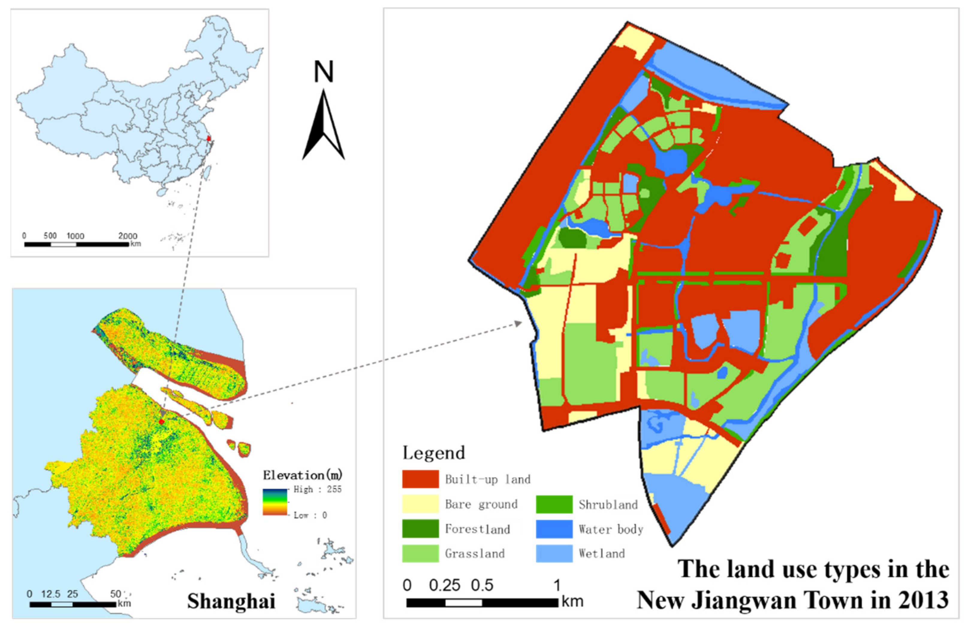
2.1. Study Area

Our study area, New Jiangwan Town, is located at 121°29′12″~121°31′47″ E, 31°18′39″~31°20′57″ N, in the northeast corner of Shanghai, China (see Figure 1). The area of New Jiangwan Town is about 6.56 km2. It has a subtropical monsoon climate with an annual average temperature of 17.6 °C and precipitation of 1173.4 mm. Before the early 20th century, complicated river networks and widespread wetlands were dominant in this region. However, since it was turned into a military airport in the 1930s, many natural areas, including forestlands, shrublands, water bodies, and wetlands, were converted into artificial constructions [48]. The airport was abandoned in 1989, and most of the constructions were demolished, leaving the ecosystem undisturbed to experience ecological succession. During this period, the region provided a superior habitat for various species, especially various birds. From 2001 to 2003, 114 bird species were observed and documented in New Jiangwan Town, accounting for approximately 29.38% of the bird species in Shanghai, despite the fact that the region’s area only took up 0.15% of Shanghai’s area [49]. However, since 2003, with rapid urban expansion, the landscape pattern has undergone dramatic changes [50]. Due to habitat loss and fragmentation during this rapid urbanization, both the richness and abundance of birds in New Jiangwan Town have been influenced significantly [51].

2.2. Data Collection

Land-use data of New Jiangwan Town were selected from raster files interpreted based on satellite images from Google Earth over seven years, 2002, 2004, 2006, 2008, 2009, 2012, and 2013. Land use was classified into seven types: built-up land, bare ground, forestland, grassland, shrubland, water bodies, and wetland. Bird observation data for 2002, 2004, 2006, 2008, 2009, 2012, and 2013 were collected from the China Bird Records Center (http://www.birdreport.cn/. accessed on 20 May 2021). There were three observation areas in our study area, the original Jiangwan airport, the Jiangwan campus of Fudan University, and a green space around the New Jiangwan Town subway station. The data were recorded by volunteer citizens and researchers under the supervision of professional ornithologists for the same seven years. The observations were conducted once per season before 2004 and then twice per year after 2004. The observers were required to keep walking at 1.0–1.5 km/h with binoculars and to take notes of birds’ movements nearby. The notes included the date, location, and the species and number of birds. According to some previous bird studies with similar species and study areas [52,53], environmental characteristics of the study areas, field observations, and previous work [51], the bird categories were classified into forest birds (birds mainly inhabiting forestland), open-area birds (birds mainly inhabiting grassland and shrubland), and water birds (birds mainly inhabiting water bodies and wetland). A detailed classification of the species and explanations of their habitat types are shown in Appendix A [51].

2.3. Methods

2.3.1. The HQI Calculated Using the InVEST Model

The InVEST model defines HQI as the potential of ecosystems to support species survival, reproduction, and activities [29]. The variations in HQI were applied to explain changes in the habitat area, which is one of the processes in habitat loss and fragmentation [54]. The formulae of the HQI are as follows: the HQI of patch x, which is in land use type j (LULCj), is given by Qxj:
Q x j = H j 1 D x j z D x j z + k z
where z and k are scaling parameters and Hj is the suitability of land use j for the species. Generally, it is considered that the suitability of natural areas is relatively high, and that of human-dominated lands is much lower [29]. In our study, the habitats were divided into three groups according to the classification of bird habitats. Forest area refers to the forestland; open area includes grassland and shrubland; water area refers to water bodies and wetland. Due to a lack of bird studies implemented using the InVEST model, all the habitat suitability values of the habitat types were set as 1 for corresponding birds, while other land-use types were set as 0, according to other habitat-quality studies [55,56]. This assumption suggested that this habitat type was the most suitable for inhabitation, activities, and reproduction of birds than other types of habitats or artificial areas.
The threat level in grid cell x of LULCj is given by Dxj, referring to the extent to which a habitat is affected by threats in the surrounding environment:
D x j = r = 1 R y = 1 Y r W r r = 1 R W r r y i r x y β x S j r
where y indexes the grid cells on 𝑟’s raster map. Wr is the relative influence weight of threat factor r on the habitat. ry is the value of the threat factor on grid y. βx is the protection level of the grid x. Sjr is the sensitivity of land j to threat factor r. irxy is the influencing weight of threat factor ry in grid y on habitat grid x. If the influence of the threat attenuates linearly with distance, the formula is:
i r x y = 1 d x y d r   m a x
If the influence of the threat decays exponentially with distance, the formula is:
i r x y = e 2.99 d r   m a x d x y
where dxy is the linear distance between habitat grid x and threat grid y, and dr max is the maximum effective distance of threat factor r. The human-dominant areas (i.e., artificial areas) tended to be regarded as threats to the natural areas. However, bare ground was also considered to have no influence on habitats in many studies [29,57]. In our study, built-up land was selected as the threat area due to the sensitivity of birds to urban areas and human activities and because the bare ground would not interfere with the birds’ inhabitation [29]. According to previous studies in similar urban areas and the characteristics of the local environment, the influence weight of the built-up land on habitats was settled as 0.7, as it includes residential areas and roads but lacks industrial areas. In addition, the maximum distance of its influence was set as 2 km. Within the influence range, the influence weight decayed exponentially [58,59]. There were various sensitivities to the threats for different habitat types, which were also settled according to previous literature and the local environment [60,61]. In our study, the water area was the most sensitive to the threat of built-up land, while the open area was the least sensitive [62]. Meanwhile, the sensitivity of natural areas to the threat was adjusted according to the characteristics of the studied species in the calculation [63]. When studying a certain bird species, the sensitivity value of the corresponding habitat type was higher than that of other habitat types. The values of habitat suitability, a threat’s influence on habitats, and the sensitivity of habitats to the threats in New Jiangwan Town from 2002 to 2013 are provided in Appendix B, Table A1. For each type of habitat, the HQI values of the grid cells were summed and averaged.

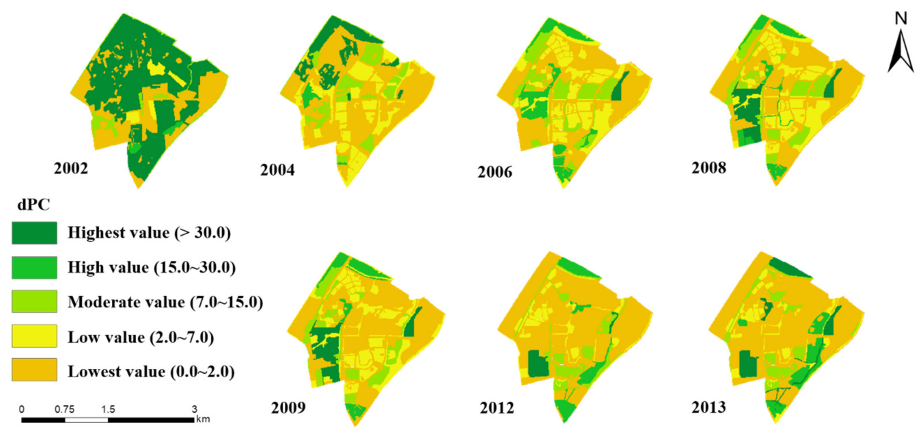
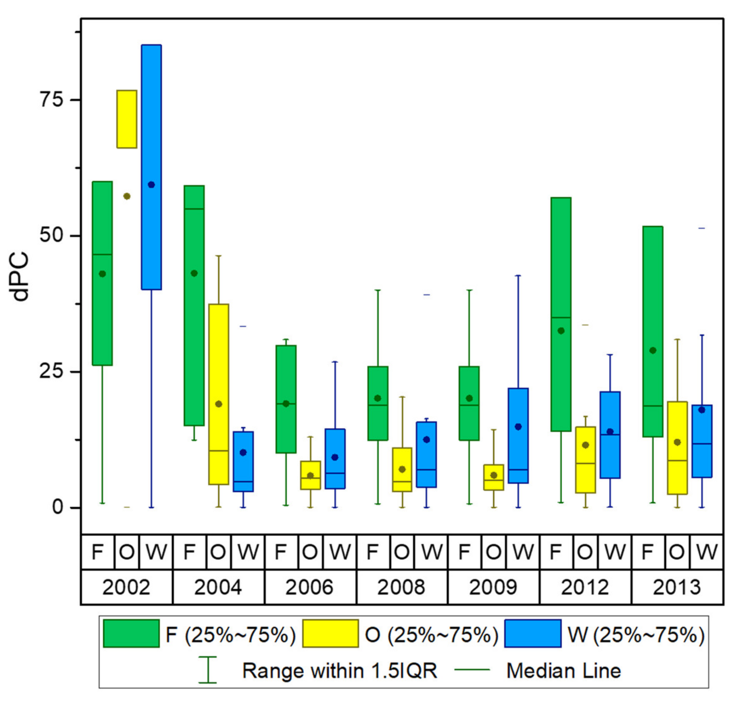
2.3.2. Habitat Connectivity Measured by the Graph-Based Connectivity Index, dPC

dPC is an index expressing habitat connectivity [47], which is explained as the probability that birds will randomly migrate from one patch to another within a certain distance threshold in our study. This index makes it possible to integrate two habitat patches that are not closely adjacent into one whole habitat area for birds, which cannot be explained by HQI. When habitat connectivity declined, the dPC fell due to the enlarging of habitat isolation. The ecological flow was interrupted as a result of the habitat change [64]. Conefor, a software for quantifying the importance of connectivity of habitat patches through graphs and availability indexes [65], was used to calculate the dPC of each habitat patch. The formula is as follows:
P C = i = 1 n j = 1 n a i × a j × p i j * A L 2
where n is the total number of habitat nodes in a landscape, ai and aj are the attributes of nodes i and j, and AL is the maximum of the attribute. If a node attribute is the area of a habitat patch, then AL is the total landscape area, comprising both habitat and non-habitat patches. p*ij is the maximum probability of all possible paths between patches i and j. A path is made up of a set of steps in which no node is visited more than once, and a step connecting two nodes does not pass by any other intermediate nodes. dPC is the PC value of a concrete node. Based on the literature, we adjusted the threshold distance settings when calculating the dPC for the habitats of different kinds of birds, depending on their migration abilities and activity ranges. The threshold distance was set at 1200 m for forest birds, 500 m for open-area birds, and 200 m for water birds [66,67,68].

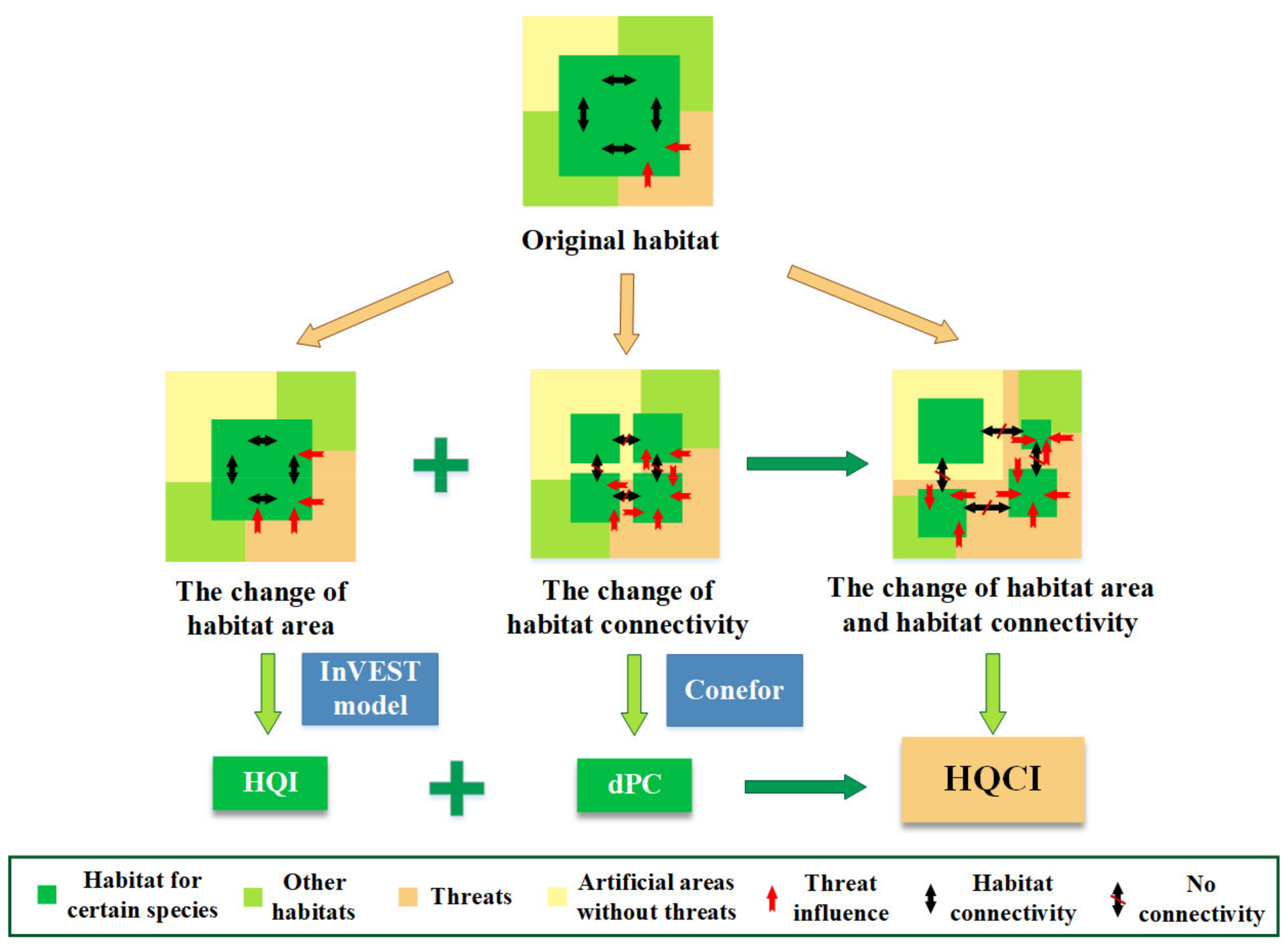
2.3.3. The New Compound Indicator Considering Both Habitat Quality and Connectivity

Both the HQI and dPC measure just one aspect of habitat change and cannot solely explain the change in habitat quality well since habitat loss and fragmentation often consist of complex processes that occur simultaneously [56,69]. When a habitat area and connectivity decline simultaneously, the habitat patches will suffer from more threats due to the enlargement of their edges, while their inner connectivity also declines. Therefore, HQCI, a combined indicator of HQI and dPC, was developed to be well associated with real-world diversity changes, as shown in Figure 2. The formula of the HQCI is as follows:
H Q C I = H Q I × d P C n o r
where dPCnor is the normalized value of the dPC. HQCI reflects the suitability, impacts of surrounding threats, and the extent of isolation of the habitats. The distribution maps and the statistical box plots of the dPC are shown in Appendix D. In each patch, classified based on the land use type, the HQI and dPC were multiplied and averaged.

2.3.4. The Calculation of Bird Diversity

Numbers, evenness, and differences of species are various aspects of biodiversity [15]. In our study, species diversity was expressed by the species richness (number of bird species observed within a year) and species abundance (mean number of each bird species observed within a year) for birds, which are two crucial indices for measuring the numbers of a species population [15,70]. Although the question of how these indices are affected by connectivity is still controversial [71], many studies have proved that habitat connectivity can affect species richness and abundance [72,73,74]. In our study, species richness and the abundance of birds were calculated directly according to the observation data.

2.3.5. The Statistical Methods

All the data, including the HQI/HQCI and bird species richness/abundance, for the three habitat types mentioned above were integrated into the analyses to explore the general ability of the HQI/HQCI to explain bird diversity. The significance of the difference between the HQI and HQCI was examined using the Mann–Whitney U-test in SPSS v.22 to ensure the comparability of the data.
Fisher’s exact test, a statistical significance test for categorical variables [75] of small samples of data [76,77], was adopted to analyze the associations between HQI/HQCI and bird species richness/abundance. Before the test, all the data were divided into two groups according to their mean values. Values greater than the mean were reclassified as 1, and those smaller than the mean were reclassified as 2.
To further explain the results of Fisher’s exact test and compare the distinctions among the different bird categories, gray correlation analysis was applied to explore the associations between the HQI/HQCI and bird species richness/bird species abundance for the different habitat types, respectively, using the SPSS v.22 tool. This was an arithmetical method based on the similarity of the variation trends between factors without limits in the sample size of data [78]. The calculation of the gray correlation degree of factor i, ri, is as follows:
r i = k = 1 n ξ i k n k = 1 ,   2 , , n ;   i = 1 ,   2 ,   m
ξ i k = min i min k x 0 k x i k + ρ max i max k x 0 k x i k x 0 k x i k + ρ max i max k x 0 k x i k
where xi(k) is the kth data of the ith factor; x0(k) is the kth data of the factor, which is used to detect correlations with other factors; m is the number of detected factors; n is the number of data points in the factor column, and ρ is an adjustable coefficient and was set at 0.5 in our study. In the gray correlation test, the correlation between HQI/HQCI and species richness/species abundance was detected separately for each bird species. Based on the results, we prepared a detailed discussion about the advantages, limitations, and future applications of the HQCI.

3. Results

3.1. Variations of Land Use Types and Bird Diversity

(1)
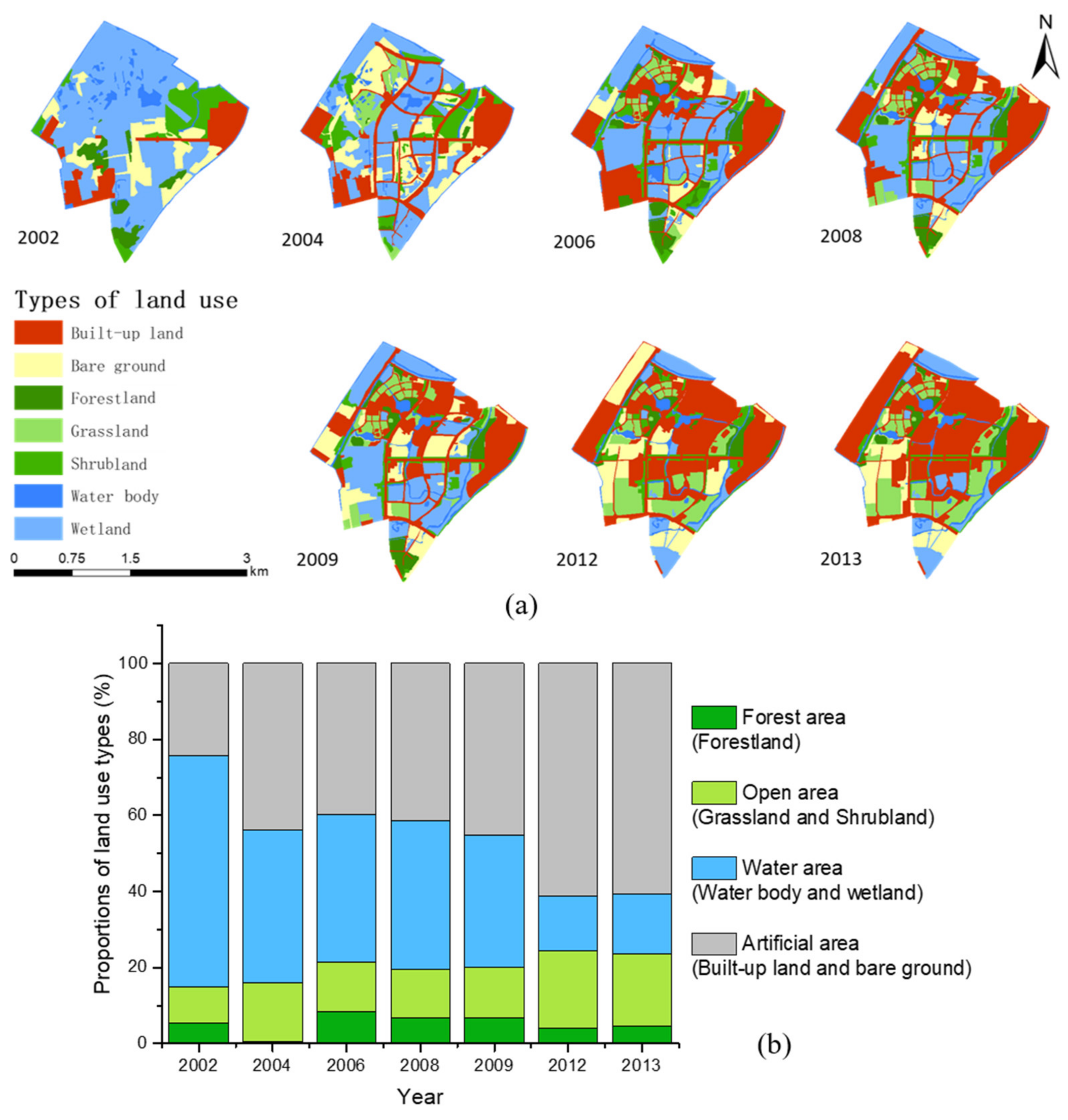
The variations of the land use types
The distributions and variations of the land use types in New Jiangwan Town from 2002 to 2013 are shown in Figure 3. Before 2004, natural areas, especially water areas, were dominant in New Jiangwan Town, accounting for 75.65% and 60.80% of the total area, respectively. With the expansion of urbanization that mainly occurred in the midland and the north, the area of the artificial area increased significantly, by 149.38%, which was mainly contributed to by built-up land, which increased by 343.11%. The water areas throughout the north and the south, as well as the forest areas in the east and the southwest, rapidly fragmented during the study period. Their areas decreased by 74.05% and 18.59%, respectively. In comparison, the open area gradually expanded and increased by 103.39% in the east and the south of the study area. In 2013, the artificial area was dominant in New Jiangwan Town, accounting for 60.74% of the region. The forest areas, open areas, and water areas accounted for 4.49%, 18.98%, and 15.78%, respectively. Most of these natural areas were scattered among the artificial areas, except for the open areas and water areas found in the southern part of New Jiangwan Town.
(2)
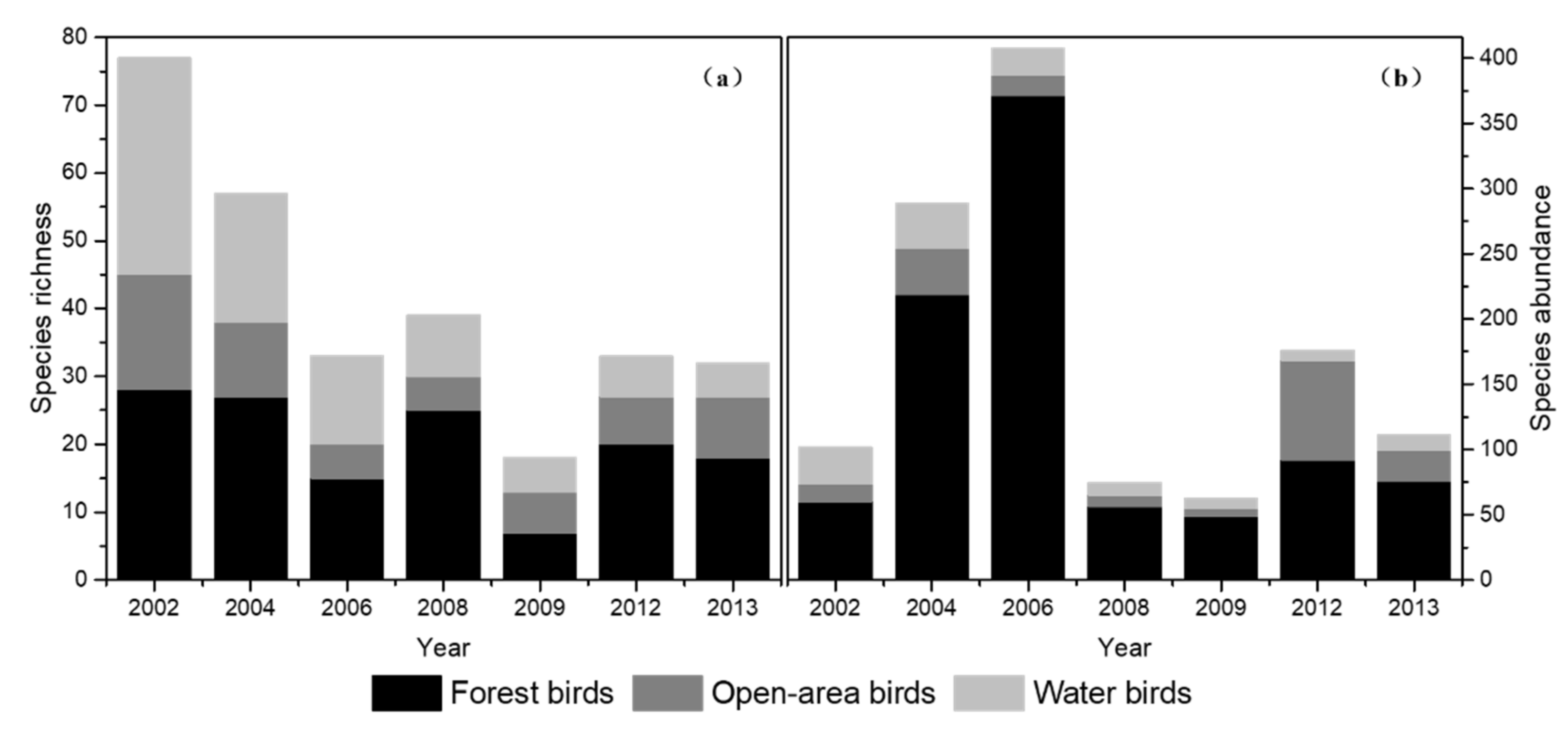
The variations of the bird diversity
The variations in species richness and abundance for three categories of birds in New Jiangwan Town are shown in Figure 4a,b, separately. From 2002 to 2013, the total species richness of birds declined by 47.4%. The total species abundance of the birds experienced severe fluctuations and increased by 72.6%. Among these, the percentage of species richness of water birds had the largest decrease, followed by open-area birds and forest birds. In contrast, the percentage of species abundance of water birds decreased by 60.0%. In comparison, that of open-area birds and forest birds increased by 76.1% and 26.4%, respectively. In 2002, the percentage of species richness of forest birds was dominant (46.0%), followed by waterbirds (30.3%) and open-area birds (23.7%). A similar situation could be observed for the percentage of species abundance. However, in 2013, the percentages of species richness and species abundance of the open-area birds exceeded those of water birds.

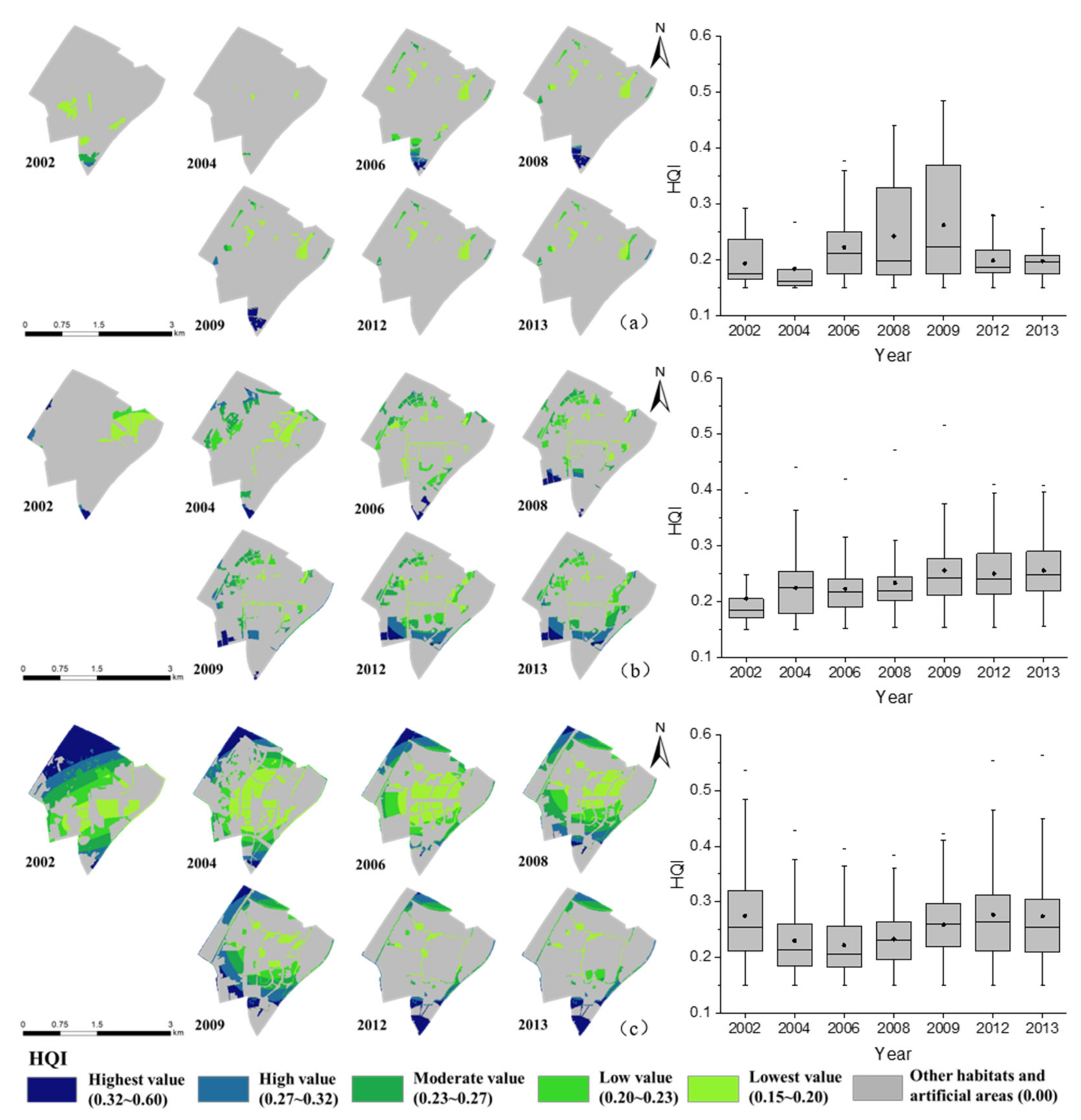
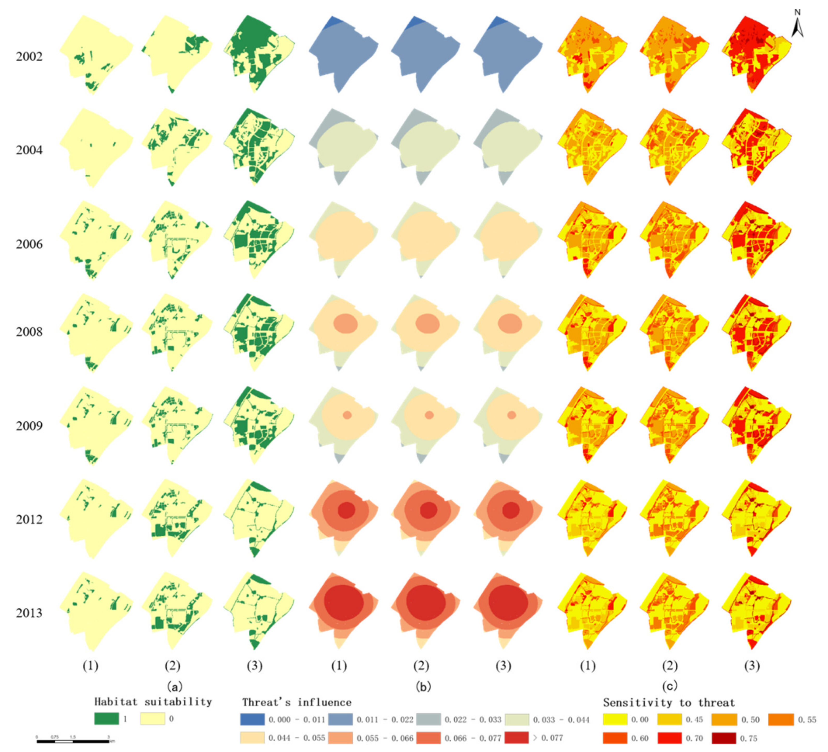
3.2. The Assessments of Habitat Quality Calculated Using the InVEST Model

The habitat quality of different habitats was calculated using the InVEST model. The variations in the habitat degradation index for three types of habitats in New Jiangwan Town from 2002 to 2013 are provided in Appendix C, Figure A2. To facilitate the comparison, HQI maps and variation box plots of the three kinds of habitats are shown in Figure 5. The values of the HQI were classified into six different ranks using the natural breaks method, including the highest HQI value (0.32–0.60), a high HQI value (0.27–0.32), a moderate HQI value (0.23–0.27), a low HQI value (0.20–0.23), the lowest HQI value (0.15–0.20), and the other habitats and artificial areas (0.00), respectively. As shown in Figure 5a–c, the HQI of all three kinds of habitats experienced fluctuations, and the changes for the forest area were the most complex. As shown in the box plots, both of the maximums in the mean HQI values for the forest areas and open areas were observed in 2009, and that of the water area appeared in 2012. The minimums in the mean HQI values for the forest areas, open areas, and water areas were observed in 2004, 2002, and 2006, respectively. This indicated that the changes in the mean HQI of the three types of habitats expressed by HQI were not exactly consistent with the variations in the corresponding land-use types.

3.2.1. Habitat Quality for the Forest Areas

According to the box-plot on the right side of Figure 5a, the average HQI value of the forest areas in 2013 did not significantly change compared with its value from 2002; it only decreased by 1.32%. This was because its total area had experienced little change over those two years. The proportion of forest areas surrounded by built-up land was low, which was an important factor that resulted in the decrease in HQI. As shown in Figure 6a, the forest areas with the highest and high HQI values were concentrated in our study area’s southern and western parts in 2002 and from 2006 to 2009. The values of HQI in the central and eastern parts were relatively low. However, the forest areas in the southern part of our study area disappeared in 2012. The great increase (by 51.36%) in the mean value of HQI from 2004 to 2009 was mainly due to the rise in the proportion of forest areas, with the highest and high HQI values. However, HQI decreased by 25.72% from 2009 to 2013, which was mainly caused by the degradation of the forest areas, with the highest and high HQI values being found in the southern part of our study area.

3.2.2. Habitat Quality for Open Areas

According to Figure 5b, the average value of the HQI for the open areas in 2013 increased by 21.82% compared with the value in 2002. As shown in Figure 3, most of the open areas were concentrated in the eastern part of our study area in 2002. Some open areas were scattered around built-up land, and they were easily influenced by human activities. Thus, the grid-like areas in the northwestern region shrank with the increase in the surrounding built-up land from 2004 to 2013. Some open areas that appeared in 2006 in the southern part had a relatively high HQI value, as they were mainly surrounded by water areas and bare grounds, which had low disturbance values. During this period, the mean value of HQI reached its highest in 2009, increasing by 12.67% from 2006, and reached its lowest in 2006, decreasing by 2.30% from 2004, as the box plot shows.

3.2.3. Habitat Quality for Water Area

According to Figure 5c, the change in the average HQI value for the water areas in 2013 was not obvious compared with the value in 2002. Still, it showed a fluctuation similar to the trend of the forest areas. In 2002, there were widespread and well-connected water areas throughout the whole region. The values of their HQI were relatively high. However, these areas were gradually marginalized and reduced in the north and the south with the expansion of urban areas, especially as of 2009. The HQI values of the remaining water areas constantly declined. The HQI values of the southwest water areas increased slightly from 2006 to 2009; however, these areas vanished in 2012. Since 2009, some small water areas recovered in the southernmost region and had the highest HQI value. Their sites were far away from the disturbance of the central built-up land. Overall, the mean value of HQI reached its lowest in 2006, decreasing by 21.22% from 2002, and its highest in 2012, increasing by 28.63% from 2006.

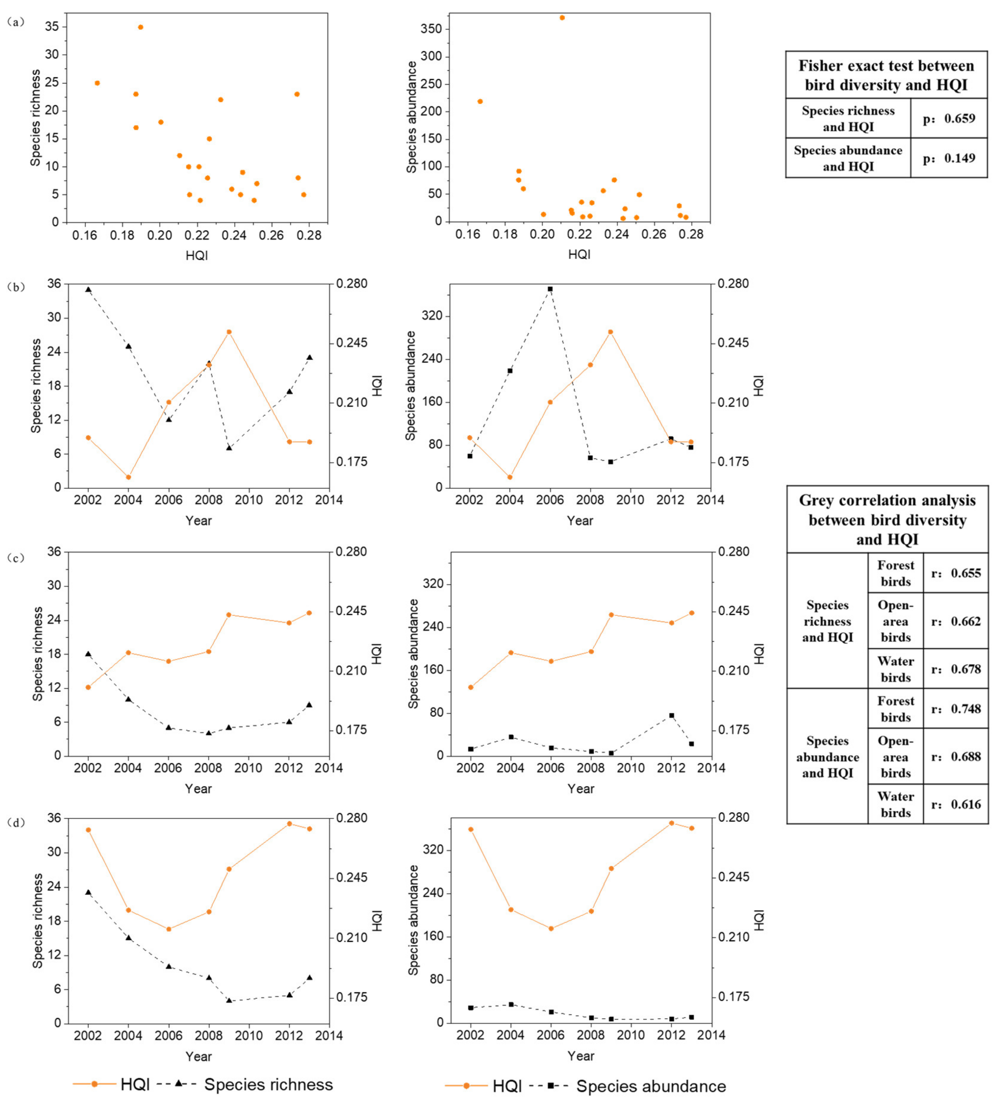
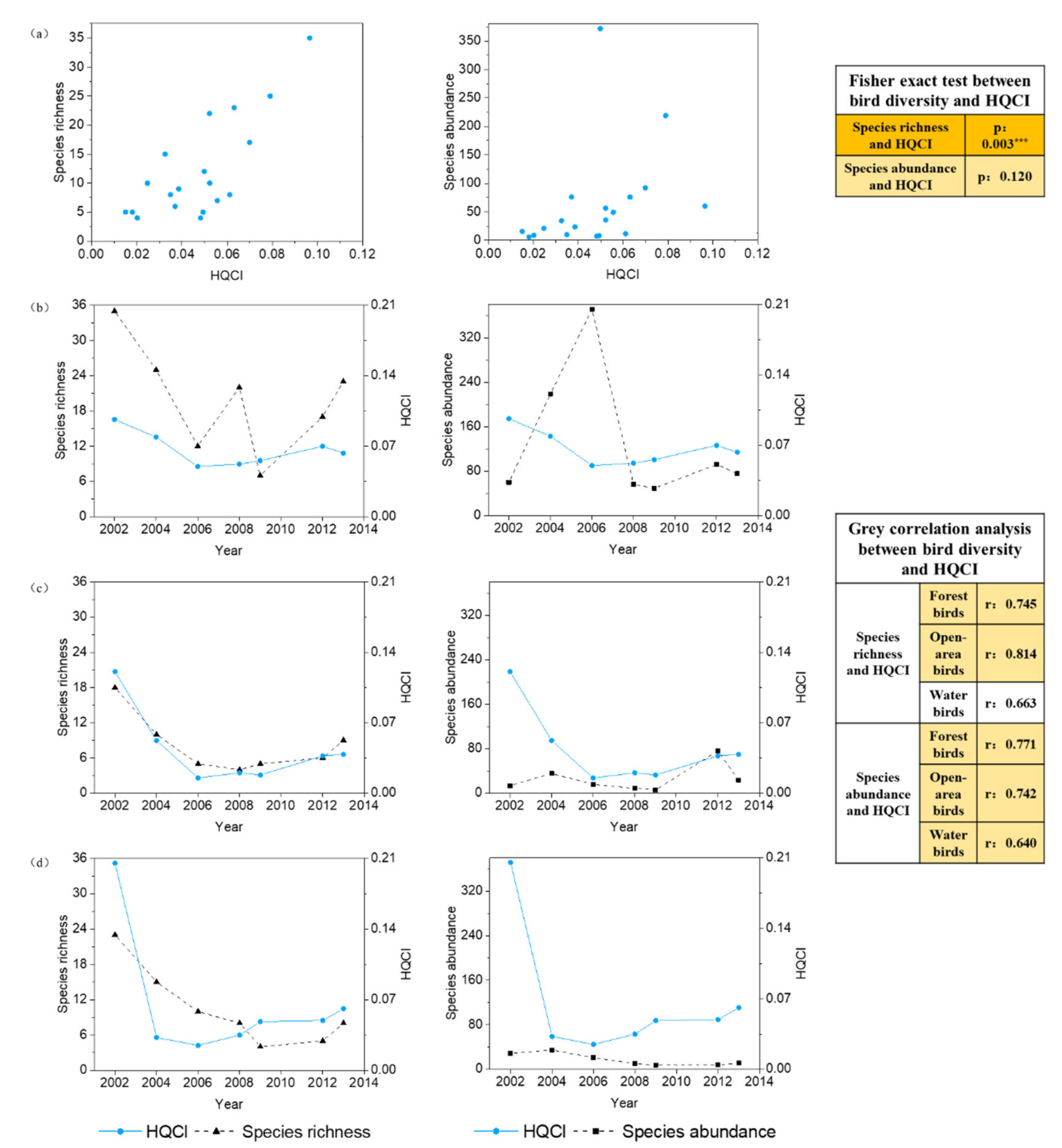
3.3. The Relationships between Bird Diversity and HQI

The variations in the species richness and abundance for the three bird categories, as well as the mean HQI values for the corresponding habitat types from 2002 to 2013, are shown in Figure 6. The Fisher’s exact test was used to examine the association between the bird diversity and HQI; however, there was no significant association between the HQIs of bird species richness or bird species abundance. In the gray correlation results for each habitat type, the gray correlation degrees between bird species richness and HQI were the largest for the water birds, followed by open-area birds and then forest birds. The gray correlation degrees between bird species abundance and HQI were the largest for forest birds, followed by open-area birds and water birds.
It seems that the HQI showed negative trends for both bird species richness and abundance (Figure 6a). Figure 6b–d shows that from 2002 to 2004, bird species richness declined, bird species abundance increased, and the HQI initially declined. When the HQI later changed, time-lags occurred between variations in the HQI and bird diversity. This period of mismatch between the HQI and species richness lasted the longest for forest birds, followed by open-area birds and water birds, which showed the same as those of the gray correlation test. The same mismatch also occurred between HQI and bird species abundance variations for all three habitat types. However, the consistency between HQI and bird species abundance was higher than that of HQI and bird species richness. In general, it could be concluded that the HQI evaluated using the InVEST model might not explain species richness and species abundance of birds well at the local scale.

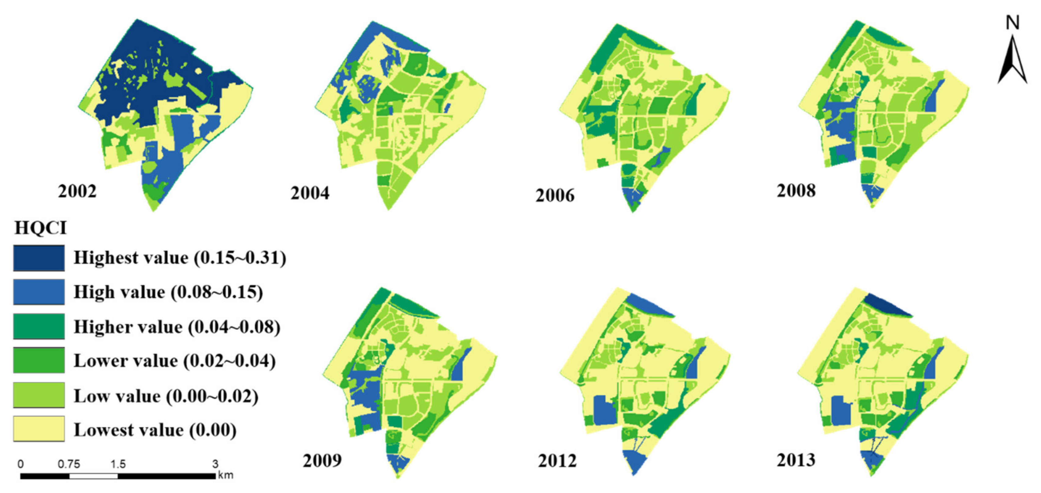
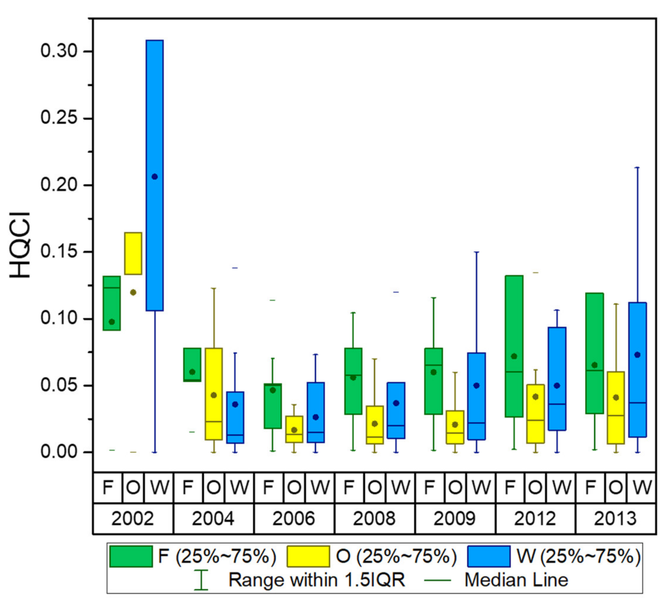
3.4. The New Compound Indicator HQCI and Its Relationship with the Bird Diversity

3.4.1. The Spatial and Temporal Variations of the New Compound Indicator HQCI

To improve the explanatory ability of HQI for variations in bird diversity, habitat connectivity was integrated to develop a new compound indicator, HQCI. The distribution maps and the statistical box-plots of the HQCI are shown in Figure 7 and Figure 8. The HQCI values were divided into six different ranks using the natural breaks method: the highest HQCI value (0.15–0.31), a high HQCI value (0.08–0.15), a higher HQCI value (0.04–0.08), a lower HQCI value (0.02–0.04), a low HQCI value (0.00–0.02) and the lowest HQCI value (0.00), respectively. As shown in Figure 7, most of the habitats in the northern and southern parts of the study area had high or the highest HQCI values in 2002, accounting for 79.12% of the natural areas, which became 24.49% in 2013. These habitats fragmented, and their HQCIs decreased to a lower level, especially from 2002 to 2006. The area with the lowest HQCI value gradually expanded during the entire study period, while areas with lower and low HQCI values increased from 2002 but then declined constantly after 2006. As shown in Figure 8, the HQCIs for the three types of habitats declined rapidly during the first two years, then fluctuated slightly until 2013. From 2002 to 2013, the mean HQCI values declined by 34.61%, 68.11%, and 70.22%, respectively. The mean HQCI value had the greatest decrease for water areas and had the smallest decline for forest areas. Comparing Figure 5 and Figure 7, the distribution of the HQCI was similar to that of the HQI, but some subtle differences existed. For example, the HQI value of the north was lower than that of the south for water areas in 2012 and 2013, while the HQCI value of the north was higher than that of the south. The dPC value of the northern water area was higher than the value of the southern part. The data of the HQI and HQCI were examined using the Mann–Whitney U test, and a significant difference (p < 0.05) was found, which proved the comparability of these two indicators.

3.4.2. Relationship between Bird Diversity and the HQCI

The variations in the species richness and the species abundance for the three bird categories and the mean HQCI values for the corresponding habitat types in New Jiangwan Town from 2002 to 2013 are shown in Figure 9. Compared with Figure 6, it can be seen that most of the associations between bird diversity and the HQCI improved. As the results of Fisher’s exact test show, there was a significant association between the HQCI and bird species richness at the 0.01 level (p < 0.01). The significance of the relationship between the HQCI and bird species abundance was also higher than that between the HQI and bird species abundance. Compared with the results shown in Figure 6, the gray correlation degrees between the bird species richness and HQCI increased by 13.7% and 22.9% for the forest areas and the open areas, respectively.
In comparison, they decreased by 2.2% for the water areas. The gray correlation degrees between the species abundance and HQCI had small increases compared with those between species and HQI for the three bird categories. This indicated that the combination of dPC performed better in explaining the variations in species richness of the forest birds and open-area birds, but not so for others.
The HQCI showed positive trends for both bird species richness and species abundance, as shown in Figure 9a, which was the opposite of the relationship between HQI and bird diversity. From Figure 9b–d, it can be seen that the consistency between bird diversity and HQCI was easier to notice than HQI, except for bird species richness in water areas (compared with Figure 6). There were still some mismatches between the trends of HQCI and bird species richness. The period of the mismatch between the HQI and species richness lasted the longest for water birds, followed by forest birds and open-area birds, which showed the results as the gray correlation test. The consistency and delays could also be found between HQCI and bird species abundance for the three types of habitats.

4. Discussion

4.1. The Problems of the Habitat Quality Indicator in Explaining Bird Diversity at the Local Scale

Biodiversity maintenance is an essential ecosystem service due to its crucial ecological functions in nature and various interactions with other ecosystem services [79]. It has been one of the most researched topics of ecosystem service studies in recent years [80]. Developing effective methods to measure biodiversity is always a crucial and difficult issue. Representing the habitat quality measured using the InVEST model, HQI mainly considers suitability for species and the extent to which these species are influenced by different land-use types [56]. The maps of HQI could easily exhibit spatial and temporal variations in habitat quality, as shown in our study. However, there are still some acknowledged problems when applying HQI in explaining some aspects of biodiversity. Our results also suggested no significant association between the HQI and species richness or species abundance of the corresponding birds in our local case. There are several potential reasons for these results.
The simplification of the ecological process is the major problem in the InVEST model [27]. The spatial heterogeneity has a crucial influence on habitat quality [81]. However, this is often ignored in the calculation of HQI [82]. Especially at the local scale, it is not enough to evaluate the richness or abundance of species simply by using the same parameters referring to previous references without considering the heterogeneity of the same types of habitats. Averaging the HQI values of habitats to explain habitat quality within a whole region is another problem of the model in explaining bird diversity. For example, as shown in Figure 5, when the open areas expanded from 2009, the overall capacity of the region for the richness and abundance of birds should have been improved with the enlarging of the habitat area [40]; however, the mean HQI value of the open area decreased instead, as such the HQI value of the newly emerged open area was very low. In addition, the habitat will be affected when surrounding habitats, which are not adjacent to it, disappear or recover [83], especially for animals [84]. The HQI ignores the interactional influence among habitat patches, which influences its ability to explain species diversity.

4.2. Applicability of the New Combined Indicator of Habitat Quality and Connectivity in Explaining Bird Diversity

Habitat connectivity has been proven to have a significant influence on biodiversity [85]. For birds, of which survival, reproduction, and activities are highly sensitive to the movements of matter and energy, variations in their populations can be easily affected by the connectivity among habitat patches [43,86,87]. As shown in Figure 9, there was a significant association between HQCI and bird species richness according to Fisher’s exact test. Meanwhile, the associations between the HQCI and species richness for forest birds and open-area birds were greatly improved by considering habitat connectivity from the gray correlation test. The association between the HQCI and species abundance was improved for all the bird categories and their integration. However, the HQCI did not perform well in explaining the variation in species richness of waterbirds in our analysis. The results indicated that different aspects of diversity for one species or one aspect of diversity for different species could differ from each other.
The differences among the birds’ migratory abilities and their adaptability to new habitats might have led to the differences in our results. Forest birds and open-area birds tend to respond faster to environmental changes due to their stronger migration abilities [88,89] since New Jiangwan Town is a small region within a city. Forest birds, able to make long-distance migrations, can find other habitats more easily when their original habitats deteriorate [90]. When the habitat quality of a region recovers again, they can migrate back to the region. However, there are fragments that hinder the process [91]. This characteristic can also be supported by the sharp fluctuation in species richness and species abundance of forest birds, shown in Figure 5a. Open area birds are supposed to gather faster in a recovered habitat than forest birds, as they tend to migrate to the adjacent breeding grounds when habitats deteriorate due to their smaller activity range [92]. Species richness and species abundance of these two bird species easily rise again when the habitat recovers. Therefore, their associations with the HQCI were higher, as shown in Figure 9. For waterbirds, the water areas they inhabit are slower to recover compared with forest areas and open areas [93]. It is also difficult to improve habitat quality within a short time for water areas. It also takes longer for water birds to adapt to a new habitat without a well-developed waterway [94]. They may not have adapted to the habitat conditions of the water areas in the region during our study period. Thus, it was harder to explain the diversity in water birds according to the HQI or HQCI than those of the other two categories of birds.

4.3. Limitations of the Present Study and Potential Guidance for Further Studies

There are still some limitations in the indicator calculation, which were not overcome in this study. Due to a lack of data, the same values of the input parameters, such as habitat suitability and the characteristics of the threats’ influences, were often used for the HQI calculation in different regions over a long period [56]. However, these characteristics often showed temporal and spatial variations in reality, such as the composition and growth conditions of vegetation [95] and the quality of water [96]. Factors, such as LAI [97], NPP [33], and some evaluating indexes for the water quality [98], are important for examining variations in habitat quality for long time periods. Their changes should be considered for improving the explaining ability of real-time habitat quality in further studies.
The influences caused by a change in bird species in the correlation analyses should not be ignored. First, birds may have different responses to an environmental change. For example, the hysteresis effect, which is a commonly recognized factor influencing biodiversity [99,100], may lead to a mismatch between bird diversity and habitat quality. Additionally, many studies have suggested that the widely studied issue of the threshold value, existing in species population dynamics, has a strong relationship with habitat quality and may be affected by habitat loss and fragmentation [101,102]. In our study, the possible existence of a threshold effect in habitat quality may also contribute to the mismatch between bird diversity and habitat quality, as observed in the variation of HQI and species richness of open-area birds. Second, the invasion of an alien species is another possible disturbance factor, often occurring in fragmented landscapes [103,104]. Especially, some urban-adapted birds that prefer to live near human-dominated areas may move into the region with the expansion of an artificial area [51]. In our study, the sharp fluctuation of all bird diversity, especially forest birds, may also be caused by increased alien birds, except for the influence of habitat quality change. Distinguishing alien species and the migration of local species is an important issue for further studies.

5. Conclusions

Explaining the variations in biodiversity at different scales has long been a hot topic. Our study provided some empirical evidence for relating the evaluating indicators of habitat quality (HQI and HQCI) to two diversity indices (species richness and species abundance) at a local scale. The associations between the overall HQI and the diversity indices and corresponding bird categories were separately not significant. Habitat connectivity expressed by dPC was then combined to develop a new index, HQCI, which showed better interpretability for the changes in bird diversity. This was the case especially for the species richness of forest birds and of open-area birds. It indicated that habitat connectivity may be an important factor for explaining the diversity of certain species at a local scale. However, the associations between HQCI and species abundance were still not significant in our study. Influences, such as time lags in a species’ response to an environmental change and the invasion of an alien species, may lead to their weak relationships. Additionally, the characteristics and the spatiotemporal variations of the internal habitat heterogeneity should be included in the model in future studies. More empirical studies should be done at different scales to provide enough evidence for applying habitat quality to be associated with biodiversity.

Author Contributions

Conceptualization: D.L. and Y.X.; data curation: D.L. and Y.X.; formal analysis: D.L. and Y.X.; funding acquisition: Y.X.; investigation: D.L.; methodology: D.L. and Y.X.; project administration: Y.X.; resources: Y.X.; software: D.L.; supervision: Y.X.; validation: Y.X.; visualization: D.L.; writing—original: D.L.; writing—review and editing: D.L., W.S., F.X., Y.Y. and Y.X. All authors have read and agreed to the published version of the manuscript.

Funding

This work was funded by the National Key Research and Development Program of China (grant number 2016YFC0502701), the Ministry of Education of Humanities and Social Science project (grant number 20YJAZH109), and the National Natural Science Foundation of China (grant number 41501194).

Institutional Review Board Statement

Not applicable.

Informed Consent Statement

Not applicable.

Data Availability Statement

Publicly available datasets were analyzed in this study. This data can be found here: [http://www.birdreport.cn/home/search/page.html], accessed on 19 May 2021].

Acknowledgments

We acknowledge the China Bird Record Center (www.birdreport.cn, accessed on 19 May 2021), the first public and professional NGO for bird records, which provided a large amount of bird census data. Thanks to the great efforts of all the volunteer citizen scientists. Thanks to Yanxia Zhao for providing the open-source bird data. Finally, we appreciate all those who contributed to bird recording activities for more than ten years and who participated in this work anonymously.

Conflicts of Interest

The authors declare no conflict of interest.

Appendix A. Classification of Species and the Explanations of the Habitat Types for Birds

NameFamilySpeciesHabitat Type
Japanese QuailPhasianidaeCoturnix japonicaO1
Common PheasantPhasianidaePhasianus colchicusF3
Mandarin DuckAnatidaeAix galericulataW1–F2
MallardAnatidaeAnas platyrhynchosW1
Spot-billed DuckAnatidaeAnas poecilorhynchaW1
Philippine DuckAnatidaeAnas luzonicaW1
Tufted duckAnatidaeAythya fuligulaW1
Eurasian hoopoeUpupidaeUpupa epopsO2
DollarbirdCoraciidaeEurystomus orientalisF2
Common KingfisherAlcedinidaeAlcedo atthisW3
Black-capped KingfisherAlcedinidaeHalcyon pileataW3
Pied KingfisherCerylidaeCeryle rudisW3
Eurasian CuckooCuculidaeCuculus canorusF2–W3
Lesser CuckooCuculidaeCuculus poliocephalusF2
Lesser CoucalCentropodidaeCentropus bengalensisF3–W3
Fork-tailed SwiftApodidaeApus pacificusO1
Indian Jungle NightjarCaprimulgidaeCaprimulgus indicusF1
Oriental Turtle DoveColumbidaeStreptopelia orientalisO2
Spotted DoveColumbidaeStreptopelia chinensisO2
White-breasted WaterhenRallidaeAmaurornis phoenicurusW3
Common MoorhenRallidaeGallinula chloropusW1–O1
Common CootRallidaeFulica atraW1
Common SnipeScolopacidaeGallinago gallinagoW3
Common GreenshankScolopacidaeTringa nebulariaW2
Green SandpiperScolopacidaeTringa ochropusW2
Wood SandpiperScolopacidaeTringa glareolaW2
Common SandpiperScolopacidaeActitis hypoleucosW2
Rufous-necked StintScolopacidaeCalidris ruficollisW2
Temminck’s StintScolopacidaeCalidris temminckiiW2
Long-toed StintScolopacidaeCalidris subminutaW2
Pheasant-tailed JacanaJacanidaeHydrophasianus chirurgusW3
Pacific Golden PloverCharadriidaePluvialis fulvaW2
Little Ringed PloverCharadriidaeCharadrius dubiusW2
Kentish PloverCharadriidaeCharadrius alexandrinusW2
Mew GulLaridaeLarus canusW3
Hen harrierAccipitridaeCircus cyaneusW1
Chinese GoshawAccipitridaeAccipiter soloensisF1
Common BuzzardAccipitridaeButeo buteoO1
Common KestrelFalconidaeFalco tinnunculusO1
Little GrebePodicipedidaeTachybaptus ruficollisW1
Great Crested GrebePodicipedidaePodiceps cristatusW1
Little EgretArdeidaeEgretta garzettaW2–F2
Gray HeronArdeidaeArdea cinereaW2–F2
Large EgretArdeidaeArdea albaW2
Intermediate EgretArdeidaeArdea intermediaW2
Cattle EgretArdeidaeBubulcus ibisW2
Chinese Pond HeronArdeidaeArdeola bacchusW2
Striated HeronArdeidaeButorides striatusW2–W3
Black-crowned Night HeronArdeidaeNycticorax nycticoraxW2–F2
Yellow BitternArdeidaeIxobrychus sinensisW3
Brown ShrikeLaniidaeLanius cristatusF3
Long-tailed ShrikeLaniidaeLanius schachF3
Azure-winged MagpieCorvidaeCyanopica cyanusF2
Black-billed MagpieCorvidaePica hudsoniaF2
Black DrongoDicruridaeDicrurus macrocercusF2
Hair-crested DrongoDicruridaeDicrurus hottentottusF1
White-throated Rock ThrushMuscicapidaeMonticola gularisF1
Scaly ThrushMuscicapidaeZoothera daumaF1
Gray-backed ThrushMuscicapidaeTurdus hortulorumF1
Japanese ThrushTurdidaeTurdus cardisF3
Eurasian BlackbirdMuscicapidaeTurdus merulaF2
Eyebrowed ThrushMuscicapidaeTurdus obscurusF1
Pale ThrushMuscicapidaeTurdus pallidusF1
Dusky ThrushMuscicapidaeTurdus eunomusO1
Gray-streaked FlycatcherMuscicapidaeMuscicapa griseistictaF1
Asian Brown FlycatcherMuscicapidaeMuscicapa dauuricaF1
Narcissus FlycatcherMuscicapidaeFicedula narcissinaF1
Mugimaki FlycatcherMuscicapidaeFicedula mugimakiF2
Blue-and-white FlycatcherMuscicapidaeCyanoptila cyanomelanaF1
BluethroatMuscicapidaeLuscinia svecicaF3
Orange-flanked Bush-RobinMuscicapidaeTarsiger cyanurusF1
Daurian RedstartMuscicapidaePhoenicurus auroreusF3
White-cheeked StarlingSturnidaeSturnus cineraceusO2
Black-collared StarlingSturnidaeGracupica nigricollisO2
Crested MynaSturnidaeAcridotheres cristatellusO1
Chinese Penduline TitRemizidaeRemiz consobrinusW3
Yellow-bellied TitParidaePardaliparus venustulusF3
Great TitParidaeParus majorF2
Black-throated TitAegithalidaeAegithalos concinnusF3
Barn SwallowHirundinidaeHirundo rusticaO1
Red-rumped SwallowHirundinidaeHirundo dauricaO1
Light-vented BulbulPycnonotidaePycnonotus sinensisF2
Himalayan Black BulbulPycnonotidaeHypsipetes leucocephalusF1
Zitting CisticolaCisticolidaeCisticola juncidisO1
Plain PriniaCisticolidaePrinia inornataW3
Manchurian Bush WarblerSylviidaeHorornis canturiansF3
Japanese Bush-WarblerSylviidaeHorornis diphoneF3
Brownish-flanked Bush-WarblerSylviidaeHorornis fortipesF3
Oriental Reed WarblerSylviidaeAcrocephalus orientalisW3
Yellow-rumped WarblerSylviidaeSetophaga coronataF3
Yellow-browed WarblerSylviidaePhylloscopus inornatusF1
Pale-legged WarblerSylviidaePhylloscopus tenellipesF1–F3
Eastern Crowned WarblerSylviidaePhylloscopus coronatusF1
Masked LaughingthrushSylviidaeGarrulax perspicillatusF3
Greater Necklaced Laughingthrush SylviidaePterorhinus pectoralisF1
HwameiSylviidaeGarrulax canorusF3
Vinous-throated ParrotbillParadoxornisSinosuthora webbianusF3
Eurasian SkylarkAlaudidaeAlauda arvensisO1
Oriental SkylarkAlaudidaeAlauda gulgulaO1
Eurasian Tree SparrowPasseridaePasser montanusF2
Forest WagtailMotacillidaeDendronanthus indicusF1
White WagtailPasseridaeMotacilla albaO1–W2
Yellow WagtailPasseridaeMotacilla flavaO1–W2
Gray WagtailPasseridaeMotacilla cinereaO1–W2
Oriental Tree PipitPasseridaeAnthus hodgsoniF2
White-rumped MuniaPasseridaeLonchura striataF3
BramblingFringillidaeFringilla montifringillaF1
Gray-capped GreenfinchFringillidaeCarduelis sinicaF2
Yellow-billed GrosbeakFringillidaeEophona migratoriaF2
Meadow BuntingFringillidaeEmberiza cioidesF2
Tristram’s BuntingFringillidaeEmberiza tristramiF3
Yellow-browed BuntingFringillidaeEmberiza chrysophrysF3
Rustic BuntingFringillidaeEmberiza rusticaF3
Yellow-throated BuntingFringillidaeEmberiza elegansF1
Yellow-breasted BuntingEmberizidaeEmberiza aureolaO1
Black-faced BuntingFringillidaeEmberiza spodocephalaF3
Where the habitat types of the birds were classified as F—forest area (F1—forest species that only use forested areas, F2—forest species that also use open areas, and F3—forest species that use boscage areas), O—open area (O1—open area species and O2—species that prefer open areas, but also use forested areas), W—water area (W1—swimming birds that use open water, W2—species that conceal themselves in marshes and aquatic areas with high grass, and W3—waders).

Appendix B. Input Parameters, Including Habitat Suitability and Sensitivity to the Threat to Different Habitat Types for Birds

Table A1. Habitat suitability and sensitivity to threats by land-use types.
Land Use TypesHabitat SuitabilitySensitivity to Threat
Forest BirdsOpen-Area BirdsWater BirdsForest BirdsOpen-Area BirdsWater Birds
Built-up land000000
Forestland1000.70.60.6
Bare ground000000
Shrubland0100.50.60.45
Water body0010.60.60.75
Wetland0010.50.50.7
Grassland0100.450.550.45

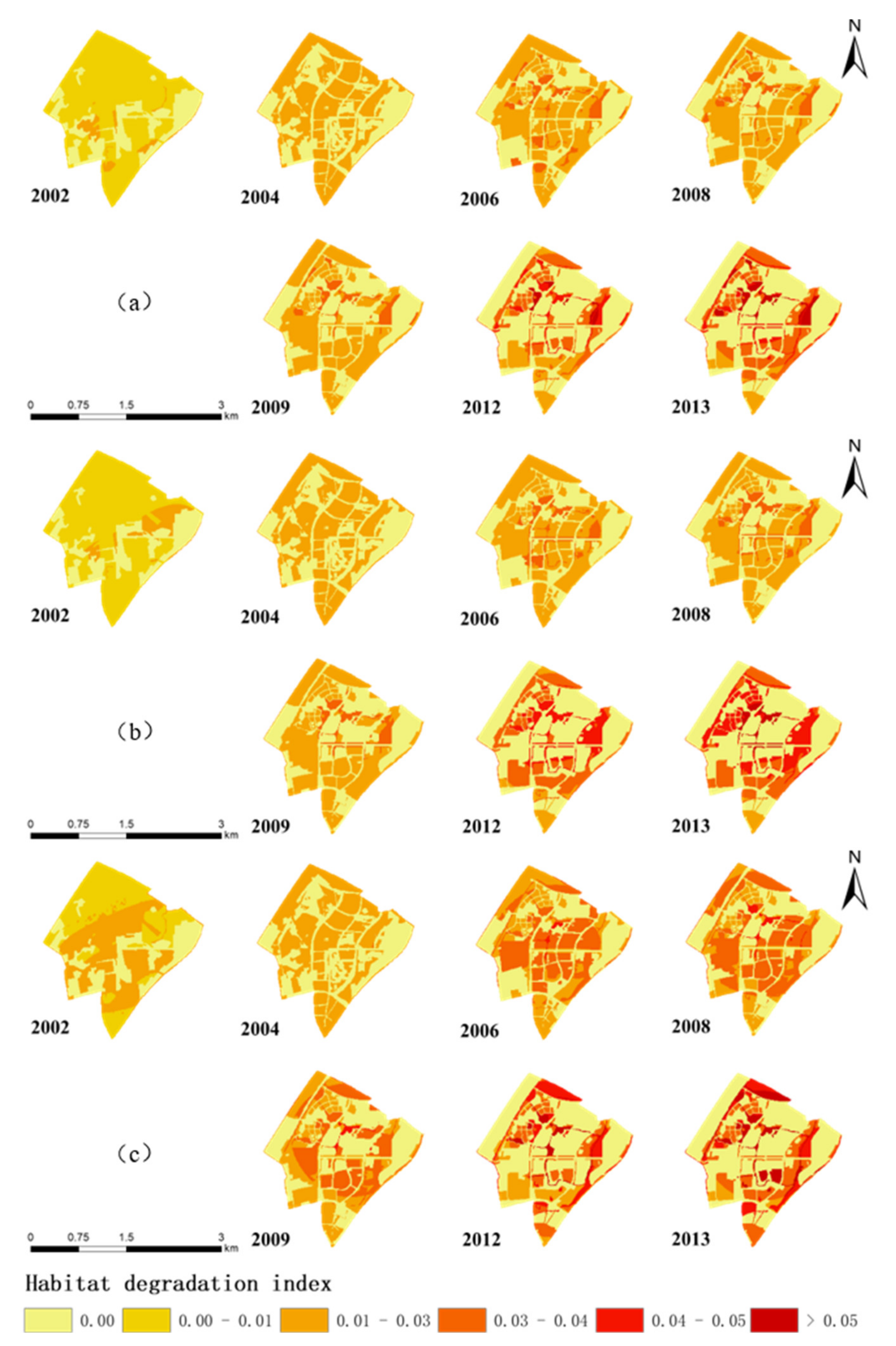
Appendix C. Input Layers for the Calculation of HQI and Variations to an Intermediate Index, the Habitat Degradation Index, for the Three Types of the Habitats in New Jiangwan Town, from 2002 to 2013

Figure A1. Habitat suitability of the habitats (a), the threat’s influence on the habitats (b), and the sensitivity of the habitats to the threat (c) in New Jiangwan Town from 2002 to 2013. (1) the forest area, (2) the open area, and (3) the water area.
Sustainability 13 05747 g0a1
Figure A2. Variations in the habitat degradation index for the three types of habitats in New Jiangwan Town from 2002 to 2013. (a) forest area, (b) open area, and (c) water area.
Sustainability 13 05747 g0a2

Appendix D. Distribution Maps and the Statistical Box-Plots of the dPC

Figure A3. Distribution of the dPC of New Jiangwan Town from 2002 to 2013.
Sustainability 13 05747 g0a3
Figure A4. Variation in the dPC of New Jiangwan Town from 2002 to 2013, where F represents the forest area, O represents the open area, and W represents the water area.
Sustainability 13 05747 g0a4

References

  1. Mace, G.M.; Norris, K.; Fitter, A.H. Biodiversity and ecosystem services: A multilayered relationship. Trends Ecol. Evol. 2012, 27, 19–26. [Google Scholar] [CrossRef]
  2. Penvern, S.; Fernique, S.; Cardona, A.; Herz, A.; Ahrenfeldt, E.; Dufils, A.; Jamar, L.; Korsgaard, M.; Kruczyńska, D.; Matray, S.; et al. Farmers’ management of functional biodiversity goes beyond pest management in organic European apple orchards. Agric. Ecosyst. Environ. 2019, 284, 106555. [Google Scholar] [CrossRef] [Green Version]
  3. Ebeling, A.; Lind, E.W.; Meyer, S.T.; Barnes, A.D.; Borer, E.T.; Eisenhauer, N.; Weisser, W.W. Contrasting effects of plant diversity on beta- and gamma-diversity of grassland invertebrates. Ecology 2020, 101, e03057-10. [Google Scholar] [CrossRef]
  4. Armenteras, D.; Rodríguez, N.; Retana, J. National and regional relationships of carbon storage and tropical biodiversity. Biol. Conserv. 2015, 192, 378–386. [Google Scholar] [CrossRef]
  5. Thorup-Kristensen, K.; Dresbøll, D.B.; Kristensen, H.L. Crop yield, root growth, and nutrient dynamics in a conventional and three organic cropping systems with different levels of external inputs and N re-cycling through fertility building crops. Eur. J. Agron. 2012, 37, 66–82. [Google Scholar] [CrossRef] [Green Version]
  6. Harrison, P.; Berry, P.; Simpson, G.; Haslett, J.; Blicharska, M.; Bucur, M.; Dunford, R.; Egoh, B.; Garcia-Llorente, M.; Geamănă, N.; et al. Linkages between biodiversity attributes and ecosystem services: A systematic review. Ecosyst. Serv. 2014, 9, 191–203. [Google Scholar] [CrossRef] [Green Version]
  7. Díaz, S.; Demissew, S.; Carabias, J.; Joly, C.; Lonsdale, M.; Ash, N.; Larigauderie, A.; Adhikari, J.R.; Arico, S.; Báldi, A.; et al. The IPBES Conceptual Framework—Connecting nature and people. Curr. Opin. Environ. Sustain. 2015, 14, 1–16. [Google Scholar] [CrossRef] [Green Version]
  8. Peng, J.; Pan, Y.; Liu, Y.; Zhao, H.; Wang, Y. Linking ecological degradation risk to identify ecological security patterns in a rapidly urbanizing landscape. Habitat Int. 2018, 71, 110–124. [Google Scholar] [CrossRef]
  9. Khoury, C.K.; Amariles, D.; Soto, J.S.; Diaz, M.V.; Sotelo, S.; Sosa, C.C.; Ramírez-Villegas, J.; Achicanoy, H.A.; Velásquez-Tibatá, J.; Guarino, L.; et al. Comprehensiveness of conservation of useful wild plants: An operational indicator for biodiversity and sustainable development targets. Ecol. Indic. 2019, 98, 420–429. [Google Scholar] [CrossRef]
  10. Heli, S.; Jyri, M.; Turo, H.; Kaisu, A. Participatory multi-criteria decision analysis in valuing peatland ecosystem services-Trade-offs related to peat extraction vs. pristine peatlands in Southern Finland. Ecol. Econ. 2019, 162, 17–28. [Google Scholar]
  11. Vaissière, A.-C.; Levrel, H.; Scemama, P. Biodiversity offsetting: Clearing up misunderstandings between conservation and economics to take further action. Biol. Conserv. 2017, 206, 258–262. [Google Scholar] [CrossRef] [Green Version]
  12. Morelli, F.; Jiguet, F.; Sabatier, R.; Dross, C.; Princé, K.; Tryjanowski, P.; Tichit, M. Spatial covariance between ecosystem services and biodiversity pattern at a national scale (France). Ecol. Indic. 2017, 82, 574–586. [Google Scholar] [CrossRef]
  13. Fisher, R.A.; Corbet, A.S.; Williams, C.B. The Relation Between the Number of Species and the Number of Individuals in a Random Sample of an Animal Population. J. Anim. Ecol. 1943, 12, 42. [Google Scholar] [CrossRef]
  14. Bartkowski, B.; Lienhoop, N.; Hansjürgens, B. Capturing the complexity of biodiversity: A critical review of economic valuation studies of biological diversity. Ecol. Econ. 2015, 113, 1–14. [Google Scholar] [CrossRef]
  15. Purvis, A.; Hector, A. Getting the measure of biodiversity. Nature 2000, 405, 212–219. [Google Scholar] [CrossRef] [PubMed]
  16. Hackman, K.O.; Gong, P. Biodiversity estimation of the western region of Ghana using arthropod mean morphospecies abundance. Biodivers. Conserv. 2017, 26, 2083–2097. [Google Scholar] [CrossRef]
  17. Ren, C.; Zhang, W.; Zhong, Z.; Han, X.; Yang, G.; Feng, Y.; Ren, G. Differential responses of soil microbial biomass, diversity, and compositions to altitudinal gradients depend on plant and soil characteristics. Sci. Total. Environ. 2018, 610–611, 750–758. [Google Scholar] [CrossRef]
  18. Yue, Y.; Zhuang, Y.; Yeh, A.G.-O.; Xie, J.-Y.; Ma, C.-L.; Li, Q.-Q. Measurements of POI-based mixed use and their relationships with neighbourhood vibrancy. Int. J. Geogr. Inf. Sci. 2017, 31, 658–675. [Google Scholar] [CrossRef] [Green Version]
  19. Mora, F. The use of ecological integrity indicators within the natural capital index framework: The ecological and economic value of the remnant natural capital of México. J. Nat. Conserv. 2019, 47, 77–92. [Google Scholar] [CrossRef]
  20. Gao, T.; Nielsen, A.B.; Hedblom, M. Reviewing the strength of evidence of biodiversity indicators for forest ecosystems in Europe. Ecol. Indic. 2015, 57, 420–434. [Google Scholar] [CrossRef]
  21. Pomerantz, A.; Peñafiel, N.; Arteaga, A.; Bustamante, L.; Pichardo, F.; Coloma, L.A.; Barrio-Amorós, C.L.; Salazar-Valenzuela, D.; Prost, S. Real-time DNA barcoding in a rainforest using nanopore sequencing: Opportunities for rapid biodiversity assessments and local capacity building. GigaScience 2018, 7, giy033. [Google Scholar] [CrossRef] [PubMed] [Green Version]
  22. Muller, F.; Lenz, R. Ecological indicators: Theoretical fundamentals of consistent applications in environmental management—Introduction. Ecol. Indic. 2006, 6, 1–5. [Google Scholar] [CrossRef]
  23. Hooper, D.U.; Chapin, F.S.; Ewel, J.J.; Hector, A.; Inchausti, P.; Lavorel, S.; Lawton, J.H.; Lodge, D.M.; Loreau, M.; Naeem, S.; et al. Effects of biodiversity on ecosystem functioning: A consensus of current knowledge. Ecol. Monogr. 2005, 75, 3–35. [Google Scholar] [CrossRef]
  24. Hansen, M.C.; Loveland, T.R. A review of large area monitoring of land cover change using Landsat data. Remote Sens. Environ. 2012, 122, 66–74. [Google Scholar] [CrossRef]
  25. Ma, L.; Sun, R.; Kazemi, E.; Pang, D.; Zhang, Y.; Sun, Q.; Zhou, J.; Zhang, K. Evaluation of Ecosystem Services in the Dongting Lake Wetland. Water 2019, 11, 2564. [Google Scholar] [CrossRef] [Green Version]
  26. Pham, H.V.; Sperotto, A.; Torresan, S.; Acuña, V.; Jorda-Capdevila, D.; Rianna, G.; Marcomini, A.; Critto, A. Coupling scenarios of climate and land-use change with assessments of potential ecosystem services at the river basin scale. Ecosyst. Serv. 2019, 40, 101045. [Google Scholar] [CrossRef]
  27. Redhead, J.W.; May, L.; Oliver, T.H.; Hamel, P.; Sharp, R.; Bullock, J.M. National scale evaluation of the InVEST nutrient retention model in the United Kingdom. Sci. Total. Environ. 2018, 610–611, 666–677. [Google Scholar] [CrossRef]
  28. Sun, X.; Crittenden, J.C.; Li, F.; Lu, Z.; Dou, X. Urban expansion simulation and the spatio-temporal changes of ecosystem services, a case study in Atlanta Metropolitan area, USA. Sci. Total. Environ. 2018, 622–623, 974–987. [Google Scholar] [CrossRef]
  29. Terrado, M.; Sabater, S.; Chaplin-Kramer, B.; Mandle, L.; Ziv, G.; Acuña, V. Model development for the assessment of terrestrial and aquatic habitat quality in conservation planning. Sci. Total. Environ. 2016, 540, 63–70. [Google Scholar] [CrossRef] [Green Version]
  30. Upadhaya, S.; Dwivedi, P. Conversion of forestlands to blueberries: Assessing implications for habitat quality in Alabaha river watershed in Southeastern Georgia, United States. Land Use Policy 2019, 89, 104229. [Google Scholar] [CrossRef]
  31. Wu, C.F.; Lin, Y.P.; Chiang, L.C.; Huang, T. Assessing highway’s impacts on landscape patterns and ecosystem services: A case study in Puli Township, Taiwan. Landsc. Urban Plan. 2014, 128, 60–71. [Google Scholar] [CrossRef]
  32. Zhang, D.; Wang, X.; Qu, L.; Li, S.; Lin, Y.; Yao, R.; Zhou, X.; Li, J. Land use/cover predictions incorporating ecological security for the Yangtze River Delta region, China. Ecol. Indic. 2020, 119, 106841. [Google Scholar] [CrossRef]
  33. Gong, J.; Xie, Y.C.; Cao, E.J.; Huang, Q.Y.; Li, H.Y. Integration of InVEST-habitat quality model with landscape pattern indexes to assess mountain plant biodiversity change: A case study of Bailongjiang watershed in Gansu Province. J. Geogr. Sci. 2019, 29, 1193–1210. [Google Scholar] [CrossRef] [Green Version]
  34. Tallis, H.; Polasky, S. Mapping and Valuing Ecosystem Services as an Approach for Conservation and Natural-Resource Management. Ann. N. Y. Acad. Sci. 2009, 1162, 265–283. [Google Scholar] [CrossRef] [PubMed]
  35. Verhagen, W.; Van Teeffelen, A.J.A.; Compagnucci, A.B.; Poggio, L.; Gimona, A.; Verburg, P. Effects of landscape configuration on mapping ecosystem service capacity: A review of evidence and a case study in Scotland. Landsc. Ecol. 2016, 31, 1457–1479. [Google Scholar] [CrossRef]
  36. Duarte, G.T.; Santos, P.M.; Cornelissen, T.G.; Ribeiro, M.C.; Paglia, A.P. The effects of landscape patterns on ecosystem services: Meta-analyses of landscape services. Landsc. Ecol. 2018, 33, 1247–1257. [Google Scholar] [CrossRef] [Green Version]
  37. Li, C.; Zhao, J. Investigating the Spatiotemporally Varying Correlation between Urban Spatial Patterns and Ecosystem Services: A Case Study of Nansihu Lake Basin, China. ISPRS Int. J. Geo-Inf. 2019, 8, 346. [Google Scholar] [CrossRef] [Green Version]
  38. Lenore, F.; Jacques, B.; Lluís, B.; Burel, F.G.; Crist, T.O.; Fuller, R.J.; Clelia, S.; Siriwardena, G.M.; Jean-Louis, M. Functional landscape heterogeneity and animal biodiversity in agricultural landscapes. Ecol. Lett. 2011, 14, 101–112. [Google Scholar]
  39. Stein, A.; Gerstner, K.; Kreft, H. Environmental heterogeneity as a universal driver of species richness across taxa, biomes and spatial scales. Ecol. Lett. 2014, 17, 866–880. [Google Scholar] [CrossRef]
  40. Fahrig, L. Effects of habitat fragmentation on biodiversity [Review]. Annu. Rev. Ecol. Evol. Syst. 2003, 34, 487–515. [Google Scholar] [CrossRef] [Green Version]
  41. Debinski, D.M.; Holt, R.D. A Survey and Overview of Habitat Fragmentation Experiments. Conserv. Biol. 2000, 14, 342–355. [Google Scholar] [CrossRef]
  42. Theodorou, P.; Radzevičiūtė, R.; Lentendu, G.; Kahnt, B.; Husemann, M.; Bleidorn, C.; Settele, J.; Schweiger, O.; Grosse, I.; Wubet, T.; et al. Urban areas as hotspots for bees and pollination but not a panacea for all insects. Nat. Commun. 2020, 11, 576. [Google Scholar] [CrossRef] [PubMed]
  43. Reis, E.; López-Iborra, G.M.; Pinheiro, R.T. Changes in bird species richness through different levels of urbanization: Implications for biodiversity conservation and garden design in Central Brazil. Landsc. Urban Plan. 2012, 107, 31–42. [Google Scholar] [CrossRef]
  44. Bregman, T.P.; Sekercioglu, C.H.; Tobias, J.A. Global patterns and predictors of bird species responses to forest fragmentation: Implications for ecosystem function and conservation. Biol. Conserv. 2014, 169, 372–383. [Google Scholar] [CrossRef]
  45. Lopes, E.V.; Mendonça, L.B.; Junior, M.A.D.S.; López-Iborra, G.M.; Dos Anjos, L. Effects of Connectivity on the Forest Bird Communities of Adjacent Fragmented Landscapes. Ardeola 2016, 63, 279–293. [Google Scholar] [CrossRef] [Green Version]
  46. Pereira, J.; Saura, S.; Jordán, F. Single-node vs. multi-node centrality in landscape graph analysis: Key habitat patches and their protection for 20 bird species in NE Spain. Methods Ecol. Evol. 2017, 8, 1458–1467. [Google Scholar] [CrossRef]
  47. Saura, S.; Pascual-Hortal, L. A new habitat availability index to integrate connectivity in landscape conservation planning: Comparison with existing indices and application to a case study. Landsc. Urban Plan. 2007, 83, 91–103. [Google Scholar] [CrossRef]
  48. Yang, Y.C.; Da, L.J.; Ji, F. Study on diversity of plant community at Jiangwan Airport, Shanghai. Shanghai Environ. Sci. 2003, 9, 615–618. (In Chinese) [Google Scholar]
  49. Jin, X.B.; Zhou, B.C.; Qin, X.K.; Cui, Z.X.; Xia, J.H.; Si, Q.; Liu, M.P. Biodiversity of the Jiangwan Airport in Shanghai. In Proceedings of the 6th National Workshop on Biodiversity Conservation and Sustainable Use, Li Jiang, China, 12–14 May 2004; Biodiversity Committee, Chinese Academy of Sciences: Li Jiang, China, 2004; pp. 1–36. (In Chinese). [Google Scholar]
  50. Yang, Y.C.; Wang, J.; Da, L.J. Diversity, spatial pattern and dynamics of vegetation under urbanization in Shanghai (II): Study on the flora of Jiangwan Airport, an abondoned land, Shanghai (In Chinese). J. East China Norm. Univ. (Nat. Sci.) 2008, 4, 40–48. [Google Scholar]
  51. Xu, X.; Xie, Y.; Qi, K.; Luo, Z.; Wang, X. Detecting the response of bird communities and biodiversity to habitat loss and fragmentation due to urbanization. Sci. Total. Environ. 2018, 624, 1561–1576. [Google Scholar] [CrossRef]
  52. Zhou, D.; Fung, T.; Chu, L. Avian community structure of urban parks in developed and new growth areas: A landscape-scale study in Southeast Asia. Landsc. Urban Plan. 2012, 108, 91–102. [Google Scholar] [CrossRef]
  53. Luan, X.F. Studies on Avian Community of Shanghai and Planning of Conservation. Ph.D. Thesis, East China Normal University Shanghai, Shanghai, China, 2003. [Google Scholar]
  54. Fahrig, L. Ecological Responses to Habitat Fragmentation Per Se. Annu. Rev. Ecol. Evol. Syst. 2017, 48, 1–23. [Google Scholar] [CrossRef]
  55. Baral, H.; Keenan, R.J.; Sharma, S.K.; Stork, N.E.; Kasel, S. Spatial assessment and mapping of biodiversity and conservation priorities in a heavily modified and fragmented production landscape in north-central Victoria, Australia. Ecol. Indic. 2014, 36, 552–562. [Google Scholar] [CrossRef]
  56. He, J.; Huang, J.; Li, C. The evaluation for the impact of land use change on habitat quality: A joint contribution of cellular automata scenario simulation and habitat quality assessment model. Ecol. Model. 2017, 366, 58–67. [Google Scholar] [CrossRef]
  57. Yang, S.; Zhao, W.; Liu, Y.; Wang, S.; Wang, J.; Zhai, R. Influence of land use change on the ecosystem service trade-offs in the ecological restoration area: Dynamics and scenarios in the Yanhe watershed, China. Sci. Total. Environ. 2018, 644, 556–566. [Google Scholar] [CrossRef]
  58. Rimal, B.; Sharma, R.; Kunwar, R.; Keshtkar, H.; Stork, N.E.; Rijal, S.; Rahman, S.A.; Baral, H. Effects of land use and land cover change on ecosystem services in the Koshi River Basin, Eastern Nepal. Ecosyst. Serv. 2019, 38, 12. [Google Scholar] [CrossRef]
  59. Wu, J.; Feng, Z.; Gao, Y.; Peng, J. Hotspot and relationship identification in multiple landscape services: A case study on an area with intensive human activities. Ecol. Indic. 2013, 29, 529–537. [Google Scholar] [CrossRef]
  60. Xu, W.Q. Effects of Landscape Pattern Dynamics on the Habitat of Migratory Waterbirds—A Case Study in National Nature Reserve of Hunan Xinxiang Yellow River Wetland. Master’s Thesis, Henan University, Kaifeng, China, 2016. (In Chinese). [Google Scholar]
  61. Liu, Y.; Zhou, Y.; Du, Y.T. Study on the spatio-temporal patterns of habitat quality and its terrain gradient effects of the middle of the Yangtze river economic belt based on InVEST model. Resour. Environ. Yangtze Basin 2019, 28, 2429–2440. (In Chinese) [Google Scholar]
  62. Li, F.; Wang, L.; Chen, Z.; Clarke, K.C.; Li, M.; Jiang, P. Extending the SLEUTH model to integrate habitat quality into urban growth simulation. J. Environ. Manag. 2018, 217, 486–498. [Google Scholar] [CrossRef] [Green Version]
  63. Sharp, R.; Tallis, H.T.; Ricketts, T.; Guerry, A.D.; Wood, S.A.; Chaplin-Kramer, R.; Vogl, A.L. InVEST Users Guide; Stanford: The Natural Capital Project: Stanford University, University of Minnesota, The Nature Conservancy, and World Wildlife Fund, Stanford, CA, USA, 2014. [Google Scholar]
  64. Mitchell, M.G.E.; Suarez-Castro, A.F.; Martinez-Harms, M.; Maron, M.; McAlpine, C.; Gaston, K.J.; Johansen, K.; Rhodes, J.R. Reframing landscape fragmentation’s effects on ecosystem services. Trends Ecol. Evol. 2015, 30, 190–198. [Google Scholar] [CrossRef] [Green Version]
  65. Volk, X.K.; Gattringer, J.P.; Otte, A.; Harvolk-Schöning, S. Connectivity analysis as a tool for assessing restoration success. Landsc. Ecol. 2018, 33, 371–387. [Google Scholar] [CrossRef]
  66. Watson, J.E.M.; Whittaker, R.J.; Freudenberger, D. Bird community responses to habitat fragmentation: How consistent are they across landscapes? J. Biogeogr. 2005, 32, 1353–1370. [Google Scholar] [CrossRef]
  67. Cadavid-Florez, L.; Laborde, J.; Mclean, D.J. Isolated trees and small woody patches greatly contribute to connectivity in highly fragmented tropical landscapes. Landsc. Urban Plan. 2020, 196, 103745. [Google Scholar] [CrossRef]
  68. Radford, J.Q.; Bennett, A.F. Thresholds in landscape parameters: Occurrence of the white-browed treecreeper Climacteris affinis in Victoria, Australia. Biol. Conserv. 2004, 117, 375–391. [Google Scholar] [CrossRef]
  69. Holzschuh, A.; Steffan-Dewenter, I.; Tscharntke, T. How do landscape composition and configuration, organic farming and fallow strips affect the diversity of bees, wasps and their parasitoids? J. Anim. Ecol. 2010, 79, 491–500. [Google Scholar] [CrossRef]
  70. Hoyer, M.V.; Canfield, D.E. Bird abundance and species richness on Florida lakes: Influence of trophic status, lake morphology, and aquatic macrophytes. Hydrobiologia 1994, 279, 107–119. [Google Scholar] [CrossRef]
  71. Fahrig, L. Rethinking patch size and isolation effects: The habitat amount hypothesis. J. Biogeogr. 2013, 40, 1649–1663. [Google Scholar] [CrossRef]
  72. Howell, C.A.; Latta, S.C.; Donovan, T.M.; Porneluzi, P.A.; Parks, G.R.; Faaborg, J. Landscape effects mediate breeding bird abundance in midwestern forests. Landsc. Ecol. 2000, 15, 547–562. [Google Scholar] [CrossRef]
  73. Thiele, J.; Kellner, S.; Buchholz, S.; Schirmel, J. Connectivity or area: What drives plant species richness in habitat corridors? Landsc. Ecol. 2018, 33, 173–181. [Google Scholar] [CrossRef]
  74. Martensen, A.C.; Ribeiro, M.C.; Banks-Leite, C.; Prado, P.I.D.K.L.D.; Metzger, J.P.W. Associations of Forest Cover, Fragment Area, and Connectivity with Neotropical Understory Bird Species Richness and Abundance. Conserv. Biol. 2012, 26, 1100–1111. [Google Scholar] [CrossRef]
  75. Kammerlander, B.; Breiner, H.-W.; Filker, S.; Sommaruga, R.; Sonntag, B.; Stoeck, T. High diversity of protistan plankton communities in remote high mountain lakes in the European Alps and the Himalayan mountains. FEMS Microbiol. Ecol. 2015, 91, fiv010. [Google Scholar] [CrossRef] [Green Version]
  76. Kaleebu, P.; Nankya, I.L.; Yirrell, D.L.; Shafer, L.A.; Kyosiimire-Lugemwa, J.; Lule, D.B.; Morgan, D.; Beddows, S.; Weber, J.; Whitworth, J.A.G. Relation between chemokine receptor use, disease stage, and HIV-1 subtypes A and D—Results from a rural Ugandan cohort. Jaids J. Acquir. Immune Defic. Syndr. 2007, 45, 28–33. [Google Scholar] [CrossRef]
  77. Angeli, S.I. Phenotype/Genotype Correlations in a DFNB1 Cohort with Ethnical Diversity. Laryngoscope 2008, 118, 2014–2023. [Google Scholar] [CrossRef] [PubMed] [Green Version]
  78. Xu, Q.; Dong, Y.-X.; Yang, R. Urbanization impact on carbon emissions in the Pearl River Delta region: Kuznets curve relationships. J. Clean. Prod. 2018, 180, 514–523. [Google Scholar] [CrossRef]
  79. Cotter, M.; Häuser, I.; Harich, F.; He, P.; Sauerborn, J.; Treydte, A.; Martin, K.; Cadisch, G. Biodiversity and ecosystem services−A case study for the assessment of multiple species and functional diversity levels in a cultural landscape. Ecol. Indic. 2017, 75, 111–117. [Google Scholar] [CrossRef]
  80. Posner, S.; Verutes, G.; Koh, I.; Denu, D.; Ricketts, T. Global use of ecosystem service models. Ecosyst. Serv. 2016, 17, 131–141. [Google Scholar] [CrossRef]
  81. Sultana, M.; Corlatti, L.; Storch, I. The interaction of imperviousness and habitat heterogeneity drives bird richness patterns in south Asian cities. Urban Ecosyst. 2020, 1–10. [Google Scholar] [CrossRef]
  82. Ruoso, L.-E.; Plant, R.; Maurel, P.; Dupaquier, C.; Roche, P.K.; Bonin, M. Reading Ecosystem Services at the Local Scale through a Territorial Approach: The Case of Peri-Urban Agriculture in the Thau Lagoon, Southern France. Ecol. Soc. 2015, 20, 11–26. [Google Scholar] [CrossRef] [Green Version]
  83. Morante-Filho, J.C.; Benchimol, M.; Faria, D. Landscape composition is the strongest determinant of bird occupancy patterns in tropical forest patches. Landsc. Ecol. 2021, 36, 105–117. [Google Scholar] [CrossRef]
  84. Prugh, L.R.; Hodges, K.E.; Sinclair, A.R.E.; Brashares, J.S. Effect of habitat area and isolation on fragmented animal populations. Proc. Natl. Acad. Sci. USA 2008, 105, 20770–20775. [Google Scholar] [CrossRef] [Green Version]
  85. Opdam, P.; Wascher, D. Climate change meets habitat fragmentation: Linking landscape and biogeographical scale levels in research and conservation. Biol. Conserv. 2004, 117, 285–297. [Google Scholar] [CrossRef]
  86. Chace, J.F.; Walsh, J.J. Urban effects on native avifauna: A review. Landsc. Urban Plan. 2006, 74, 46–69. [Google Scholar] [CrossRef]
  87. Ramos, D.L.; Pizo, M.A.; Ribeiro, M.C.; Cruz, R.S.; Morales, J.M.; Ovaskainen, O. Forest and connectivity loss drive changes in movement behavior of bird species. Ecography 2020, 43, 1203–1214. [Google Scholar] [CrossRef]
  88. Newbold, T.; Scharlemann, J.P.W.; Butchart, S.H.M.; Şekercioğlu, Ç.H.; Alkemade, R.; Booth, H.; Purves, D.W. Ecological traits affect the response of tropical forest bird species to land-use intensity. Proc. R. Soc. B Biol. Sci. 2013, 280, 20122131. [Google Scholar] [CrossRef] [Green Version]
  89. Ribeiro, I.; Proença, V.; Serra, P.; Palma, J.; Domingo-Marimon, C.; Pons, X.; Domingos, T. Remotely sensed indicators and open-access biodiversity data to assess bird diversity patterns in Mediterranean rural landscapes. Sci. Rep. 2019, 9, 6826. [Google Scholar] [CrossRef] [PubMed] [Green Version]
  90. VanderWerf, E.A. Demography of hawai’i ‘elepaio: Variation with habitat disturbance and population density. Ecology 2004, 85, 770–783. [Google Scholar] [CrossRef]
  91. Belisle, M.; Desrochers, A.; Fortin, M.J. Influence of forest cover on the movements of forest birds: A homing experiment. Ecology 2001, 82, 1893–1904. [Google Scholar] [CrossRef]
  92. Partridge, D.R.; Clark, J.A. Urban green roofs provide habitat for migrating and breeding birds and their arthropod prey. PLoS ONE 2018, 13, e0202298. [Google Scholar] [CrossRef] [PubMed]
  93. Maleki, S.; Soffianian, A.R.; Koupaei, S.S.; Pourmanafi, S.; Saatchi, S. Wetland restoration prioritizing, a tool to reduce negative effects of drought; An application of multicriteria-spatial decision support system (MC-SDSS). Ecol. Eng. 2018, 112, 132–139. [Google Scholar] [CrossRef]
  94. Li, D.; Chen, S.; Lloyd, H.; Zhu, S.; Shan, K.; Zhang, Z. The importance of artificial habitats to migratory waterbirds within a natural/artificial wetland mosaic, Yellow River Delta, China. Bird Conserv. Int. 2013, 23, 184–198. [Google Scholar] [CrossRef] [Green Version]
  95. Shreeve, T.G.; Dennis, R.L.H. Landscape scale conservation: Resources, behaviour, the matrix and opportunities. Lepid. Conserv. Chang. World 2010, 15, 261–270. [Google Scholar] [CrossRef]
  96. Xie, Y.; Yu, X.; Ng, N.C.; Li, K.; Fang, L. Exploring the dynamic correlation of landscape composition and habitat fragmentation with surface water quality in the Shenzhen river and deep bay cross-border watershed, China. Ecol. Indic. 2018, 90, 231–246. [Google Scholar] [CrossRef]
  97. Pfeifer, M.; Boyle, M.J.; Dunning, S.; Olivier, P.I. Forest floor temperature and greenness link significantly to canopy attributes in South Africa’s fragmented coastal forests. PeerJ. 2019, 7, e6190. [Google Scholar] [CrossRef]
  98. Calderon, M.R.; Almeida, C.A.; González, P.; Jofré, M.B. Influence of water quality and habitat conditions on amphibian community metrics in rivers affected by urban activity. Urban Ecosyst. 2019, 22, 743–755. [Google Scholar] [CrossRef]
  99. Daw, T.M.; Hicks, C.C.; Brown, K.; Chaigneau, T.; Januchowski-Hartley, F.A.; Cheung, W.W.L.; Rosendo, S.; Crona, B.; Coulthard, S.; Sandbrook, C.; et al. Elasticity in ecosystem services: Exploring the variable relationship between ecosystems and human well-being. Ecol. Soc. 2016, 21, 11–13. [Google Scholar] [CrossRef]
  100. Buschke, F.T.; Esterhuyse, S.; Kemp, M.E.; Seaman, M.T.; Brendonck, L.; Vanschoenwinkel, B. The dynamics of mountain rock pools—Are aquatic and terrestrial habitats alternative stable states? Acta Oecologica 2013, 47, 24–29. [Google Scholar] [CrossRef]
  101. Boesing, A.L.; Nichols, E.; Metzger, J.P. Biodiversity extinction thresholds are modulated by matrix type. Ecography 2018, 41, 1520–1533. [Google Scholar] [CrossRef] [Green Version]
  102. Fahrig, L. How much habitat is enough? Biol. Conserv. 2001, 100, 65–74. [Google Scholar] [CrossRef]
  103. Sakai, A.K.; Allendorf, F.W.; Holt, J.S.; Lodge, D.M.; Molofsky, J.; With, K.A.; Baughman, S.; Cabin, R.J.; Cohen, J.E.; Ellstrand, N.C.; et al. The Population Biology of Invasive Species. Annu. Rev. Ecol. Syst. 2001, 32, 305–332. [Google Scholar] [CrossRef] [Green Version]
  104. Smith, D.A.E.; Si, X.; Smith, Y.C.E.; Kalle, R.; Ramesh, T.; Downs, C.T. Patterns of avian diversity across a decreasing patch-size gradient in a critically endangered subtropical forest system. J. Biogeogr. 2018, 45, 2118–2132. [Google Scholar] [CrossRef]
Figure 1. Location of the study area.
Sustainability 13 05747 g001
Figure 2. Conceptual view of the three processes in habitat loss and fragmentation, expressed by three indices.
Sustainability 13 05747 g002
Figure 3. Variations in land-use types in New Jiangwan Town from 2002 to 2013: (a) spatiotemporal distribution maps and (b) stacked-bar charts of the proportions.
Sustainability 13 05747 g003
Figure 4. Variations in the species richness (a) and the species abundance (b) of the three bird categories in New Jiangwan Town from 2002 to 2013.
Sustainability 13 05747 g004
Figure 5. Variations in the HQI of the three types of habitats in New Jiangwan Town from 2002 to 2013: (a) forest areas, (b) open areas, and (c) water areas.
Sustainability 13 05747 g005
Figure 6. Relationship between species richness and species abundance for three bird categories and the mean HQI values for the according to habitat types: (a) all data in the three bird categories, (b) forest birds, (c) open-area birds, and (d) water birds. The indexes in the results: p: the significance index of ‘s exact test; r: the gray correlation degree.
Sustainability 13 05747 g006
Figure 7. Distribution of the HQCI of New Jiangwan Town from 2002 to 2013.
Sustainability 13 05747 g007
Figure 8. Variation in the HQCI of New Jiangwan Town from 2002 to 2013, where F represents the forest areas, O represents the open areas, and W represents the water areas.
Sustainability 13 05747 g008
Figure 9. Relationship between species richness and species abundance for three bird categories and the mean HQCI values according to habitat type: (a) all the data for the three bird categories; (b) forest birds; (c) open-area birds; (d) water birds. The indexes in the results: p: the significance index of Fisher’s exact test; r: the gray correlation degree. *** represents a significant correlation at the 0.01 level. The gold block indicates the association between the HQCI and the diversity index improved compared with the HQI and is significant in Fisher’s exact test. The pale-yellow block indicates the associations between the HQCI and the diversity indexes improved compared with the HQI but is not yet significant. While the block with no color indicates that the correlation has not been improved compared to before.
Sustainability 13 05747 g009
Publisher’s Note: MDPI stays neutral with regard to jurisdictional claims in published maps and institutional affiliations.

