Construction Method of a Guaranteed Grid Considering the Specific Recovery Process


Abstract
:1. Introduction
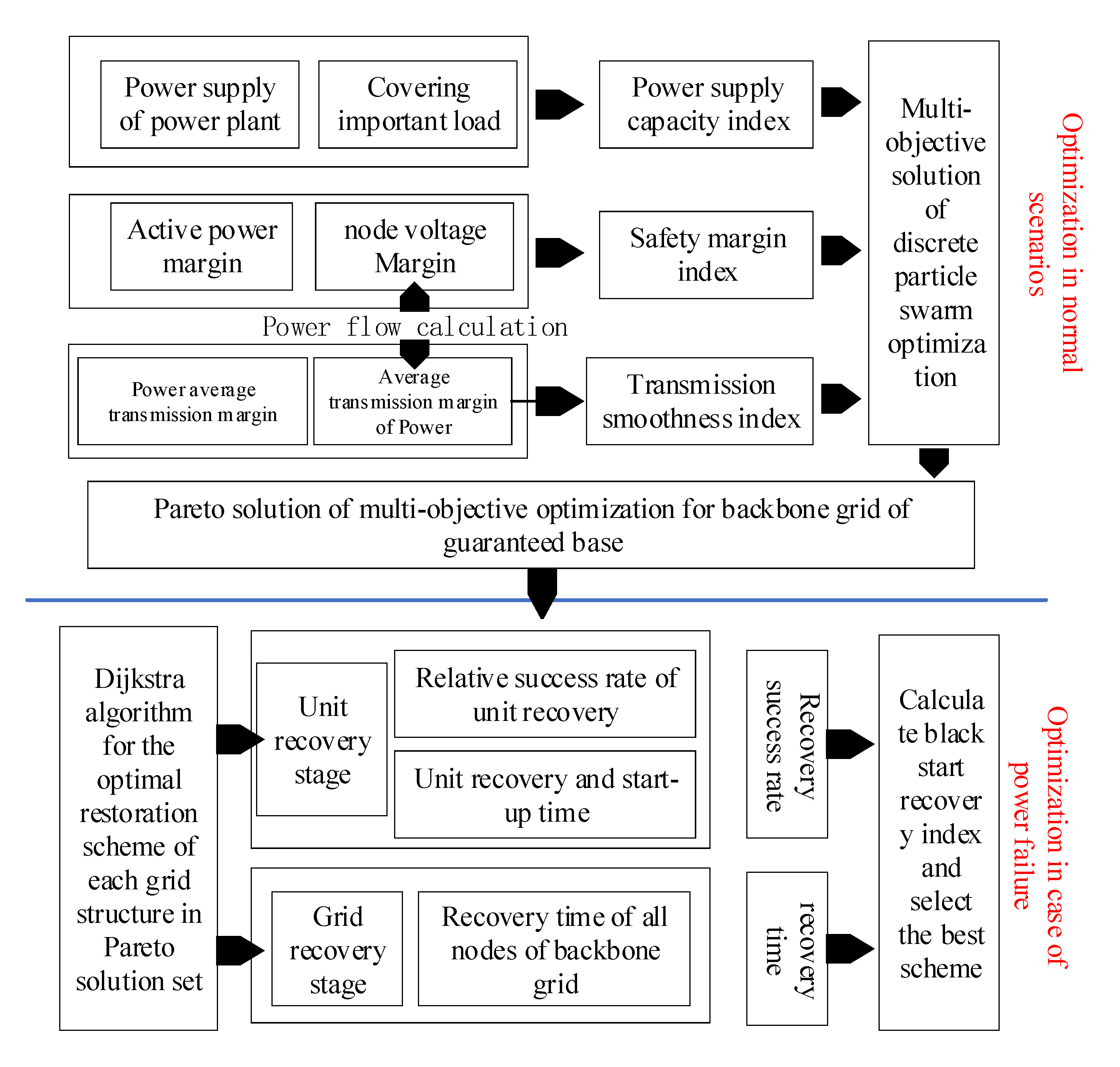
2. Overall Research Framework
- (1)
- The power supply capacity is reflected in that the backbone grid should be able to meet the important load demand, so the grid should select the access to the important load according to the load and the user’s importance level. At the same time, sufficient power supply should be reserved in order to ensure the power balance.
- (2)
- The smooth transmission reflects the difference between transmission power and the upper limit of transmission power in the electric wire. The load in the grid is largely reserved. In contrast to load retention, the backbone grid lines are greatly reduced, which leads to the increase of line burden and the extreme occurrence of power flow overrun and transmission congestion.
- (3)
- The ample safety margin aims to ensure that the backbone grid can operate stably for a period of time. When the active and reactive power in the backbone grid is sufficient, the system has a strong ability to deal with sudden small disturbances. Therefore, the safety margin is quantified as the margin between the electrical quantity and the limit operation state.
3. Optimization Model of the Backbone Grid Structure with Recovery Capability
3.1. Optimization of the Backbone Grid Structure in the Normal Scenario
3.1.1. Objective Function
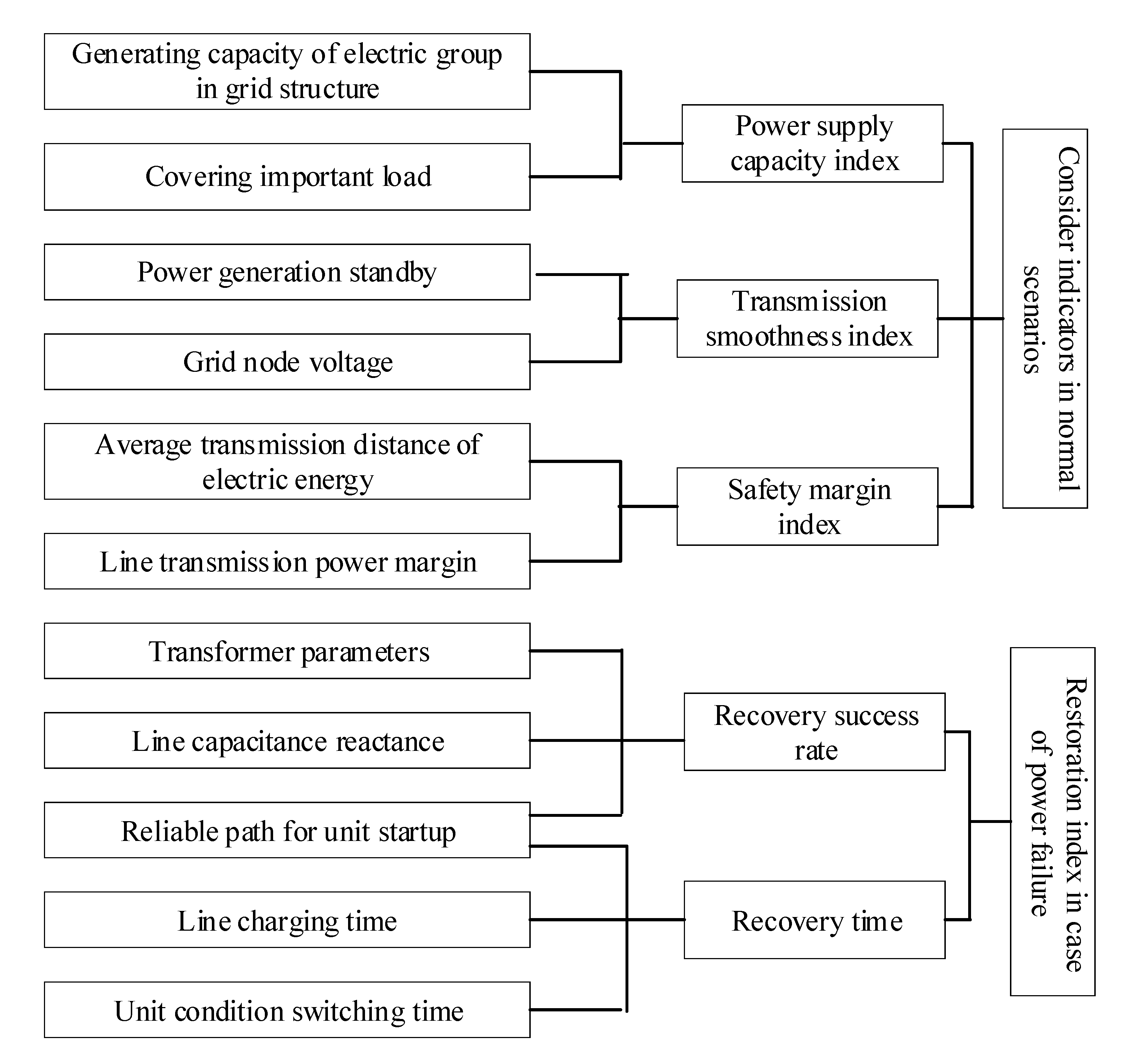
Power Supply Capacity Index
Safety Margin Index
Transmission Smoothness Index
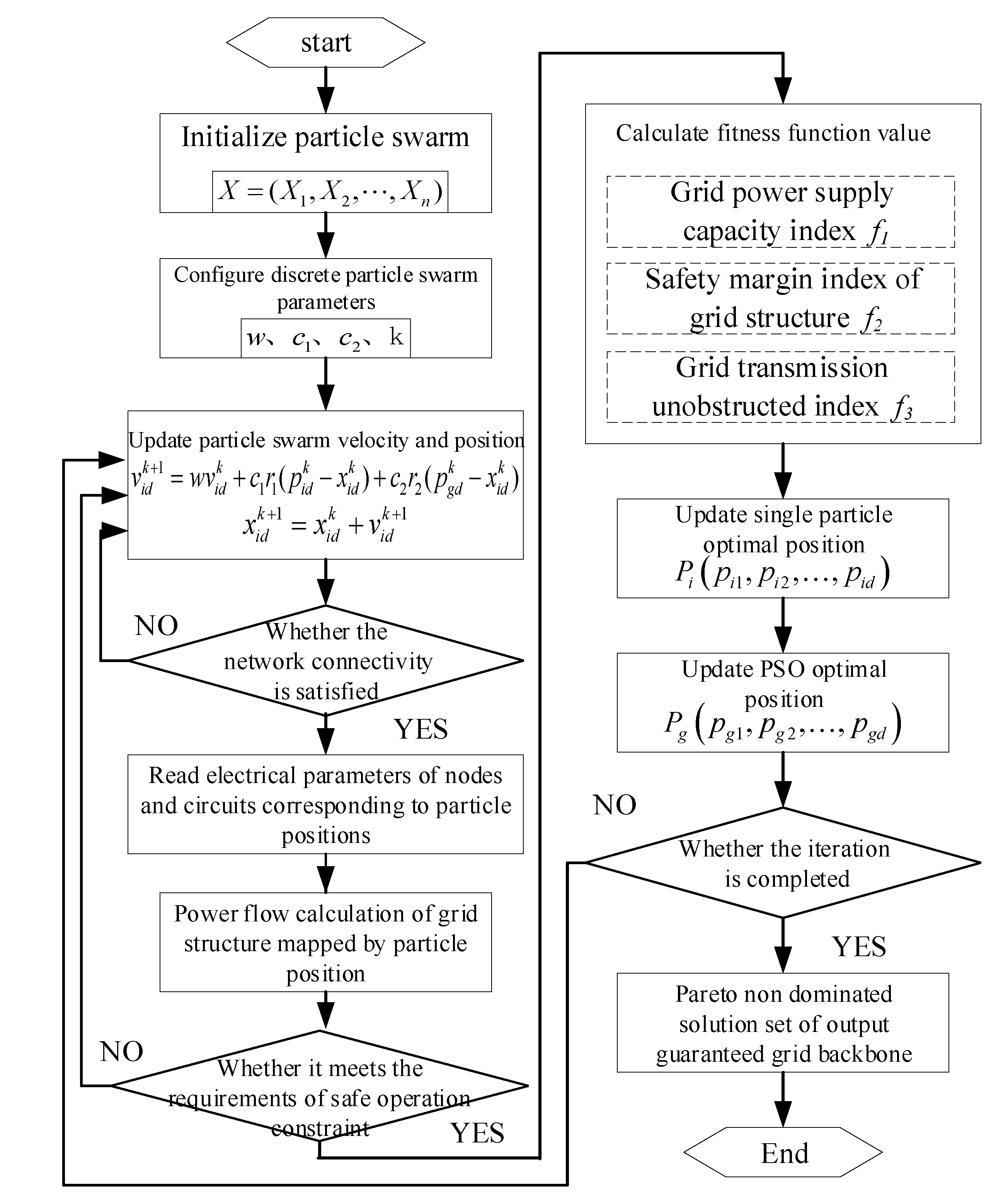
3.1.2. Multi-Objective Optimization Solution
- (1)
- When initializing a particle swarm , the position coordinate of each individual in the particle swarm is ; dimension d is equal to the number of branches of the original grid. In the discrete particle swarm algorithm, the value of each dimension of the position variables of all particles is limited to 0 or 1.
- (2)
- According to Lin et al. [26], the speed and position of the particles are updated according to Equations (11) and (12), respectively:
- (3)
- Check the validity of the updated particles. Because this is a graph theory problem, we must judge the connectivity of the branch and node set corresponding to the particle position. If it is connected, it is an effective particle—go to step 4); If it is not connected, it is an invalid particle—go back to step 2) after transforming the invalid particle.
- (4)
- According to the particle position, we can determine the branch, node set and grid structure. After the power flow calculation, the node voltage and power flow distribution are obtained. Judge whether the constraints of a safe and stable operation of the power system are met. If so, go to step 5). Otherwise, return to step 2) and regenerate new particles.
- (5)
- According to the results of the power flow calculation and basic data, the fitness function value is calculated by the optimization objective function of Equation (1), so as to update the particle optimal position and particle swarm optimal position.
- (6)
- If the number of iterations is reached, the iteration is terminated and the result of the grid optimization, which is the non-dominated solution set of grid Pareto with strong transmission capacity and full reliability. Otherwise, skip to step 2) and continue to perform the particle update.
3.2. Re-Optimization Based on the Recovery Capability in the Outage Scenario
3.2.1. Objective Function Considering the Recovery Ability of the Grid Structure
Recovery Success Rate Fable
Recovery Time
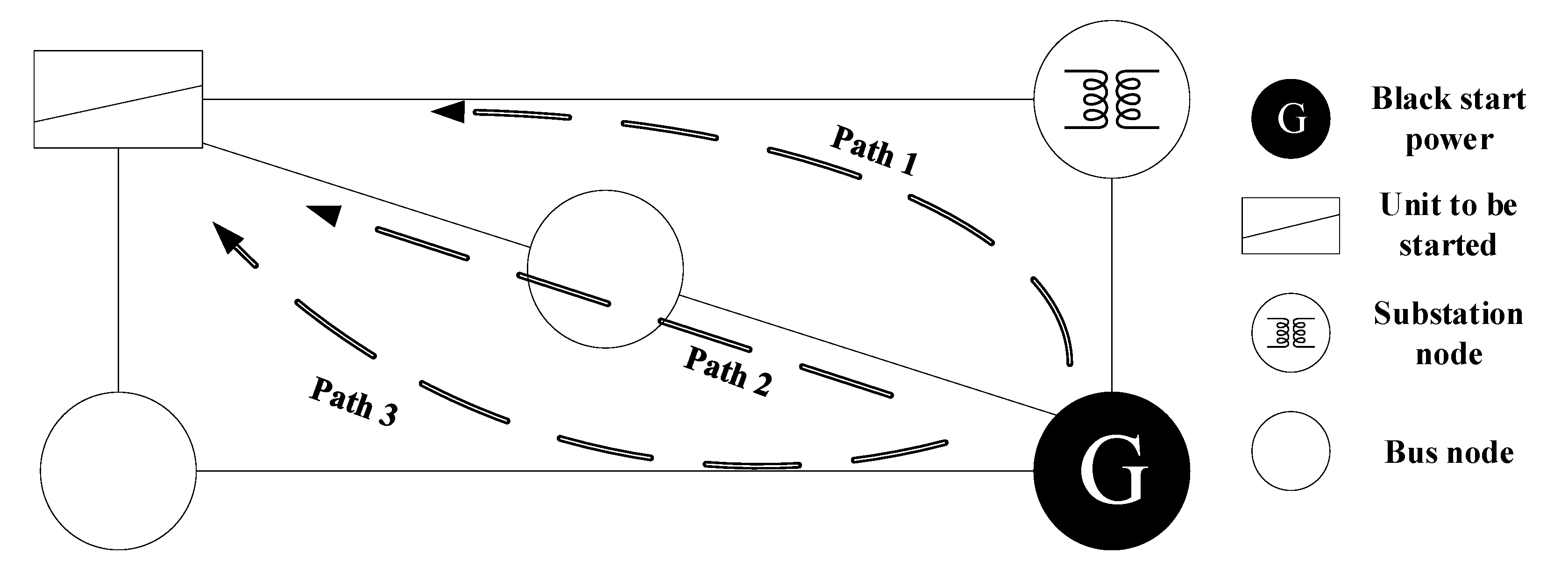
3.2.2. Optimal Recovery Path
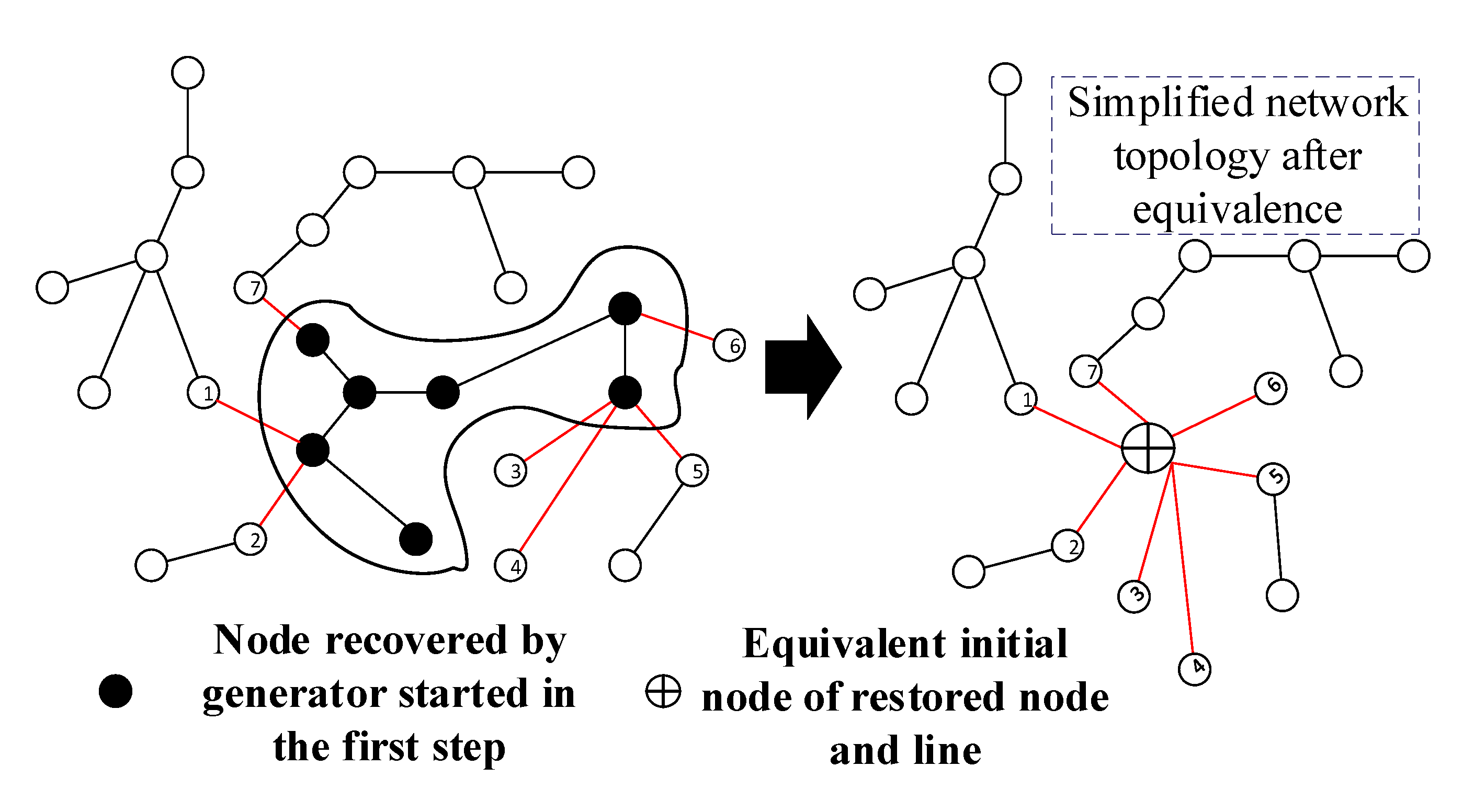
- (1)
- Extract a network topology map of a grid in Pareto’s non-dominated solution set. Assign the sum of the inverse number of transformer exponents at both ends of the line and the unit value of capacitive reactance of the line itself as the line length. The Dijkstra algorithm searches for the shortest path. Calculate and according to the path.
- (2)
- Confirm that the nodes and lines involved in the optimal path are equivalent to the initial nodes. The sum of the recovery time of the line and the equipment at both ends of the line is assigned as the line length. The Dijkstra algorithm searches for the farthest path and calculates .
- (3)
- Calculate the black start recovery index. Update the current optimal solution. Determine whether to analyze all grids in Pareto’s non-dominated solution set. If yes, the optimal grid structure will be output; otherwise, skip to 1) and continue searching.
4. Example Analysis
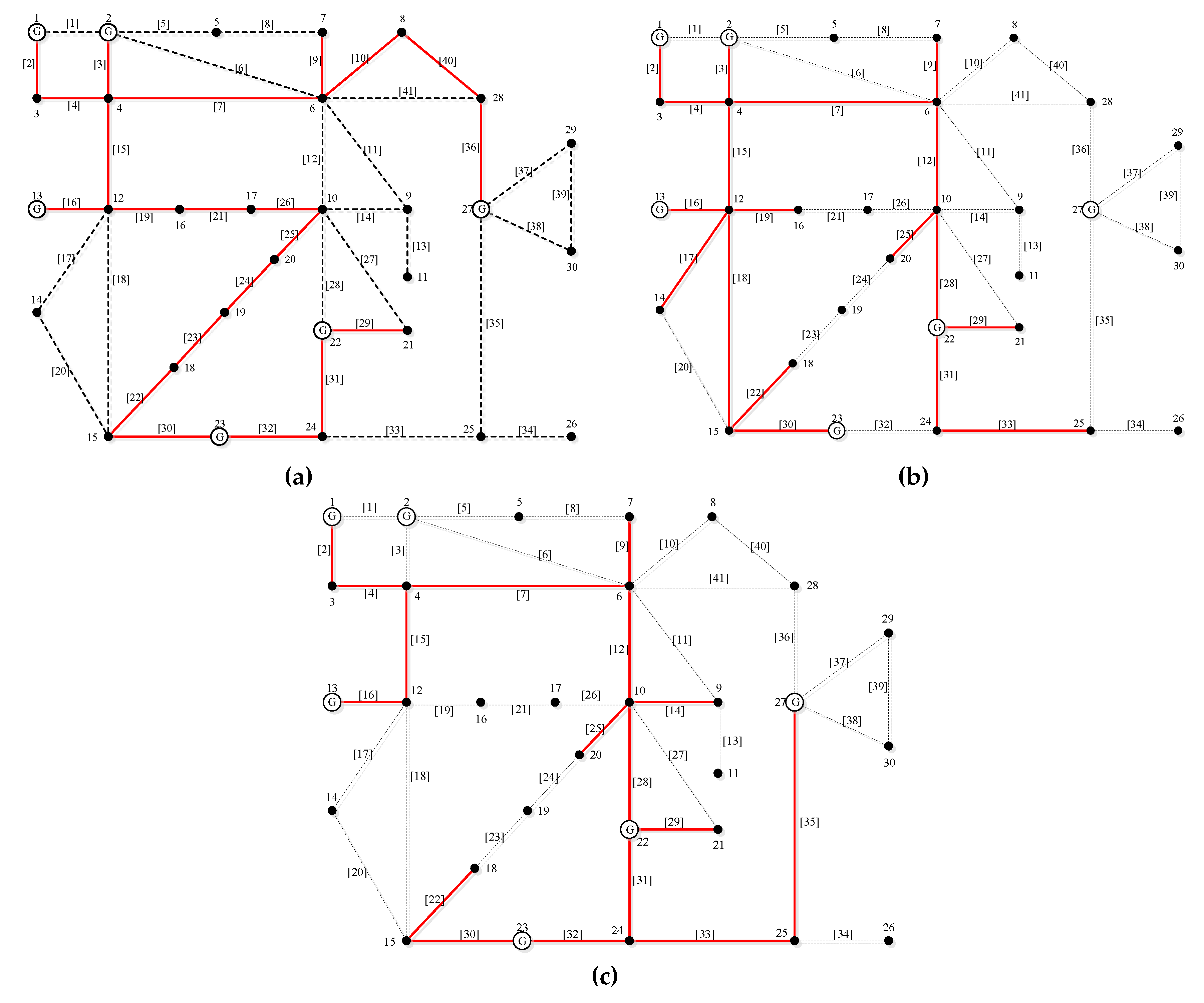
4.1. An Example Analysis of the IEEE (Institute of Electrical and Electronics Engineers)-30 Node System
4.1.1. Optimization of the Backbone Grid Structure in the Normal Scenario
4.1.2. Optimization of the Recovery Performance of the Backbone Grid Considering the Minimum Guarantee
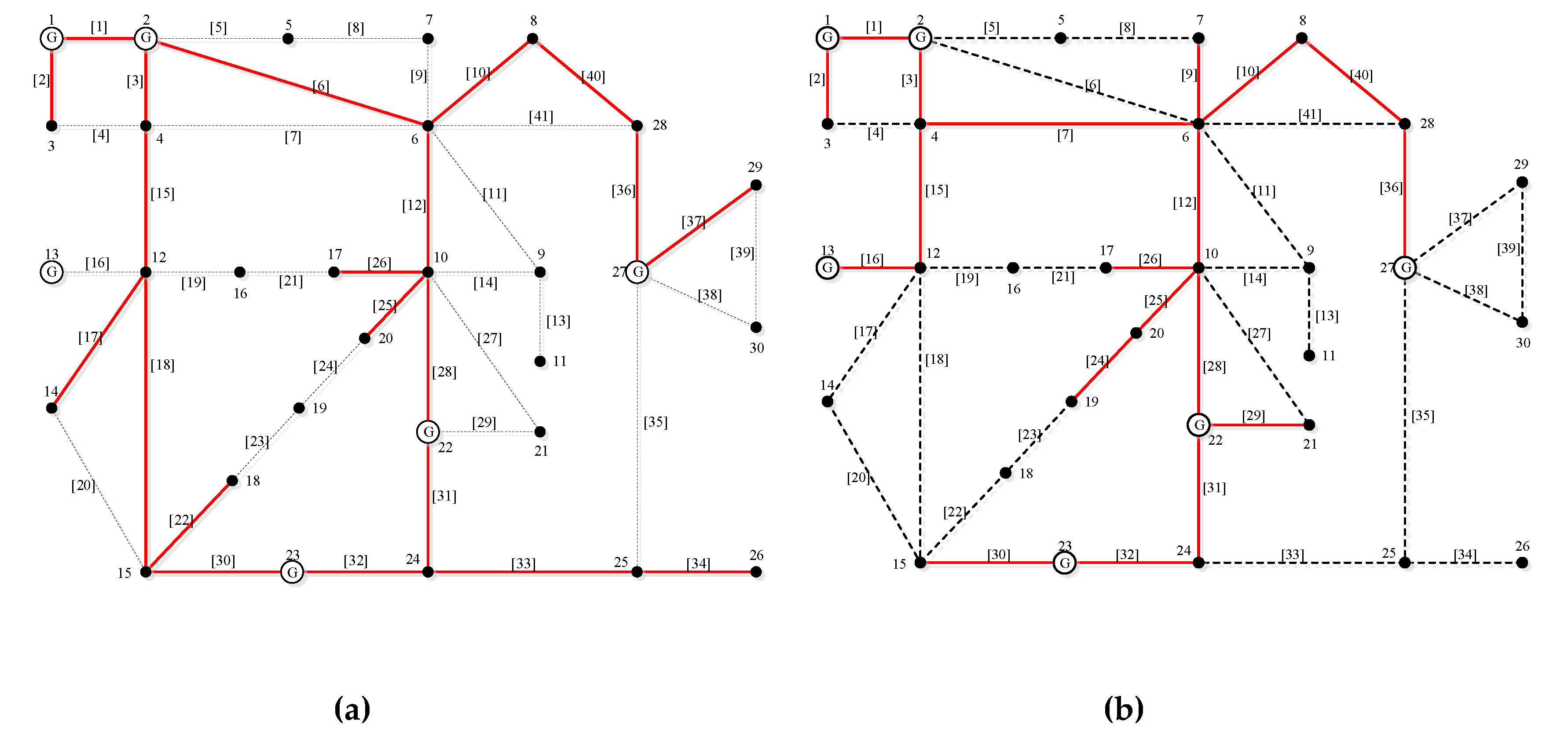
4.2. Comparative Analysis of Different Black Start Power Positions
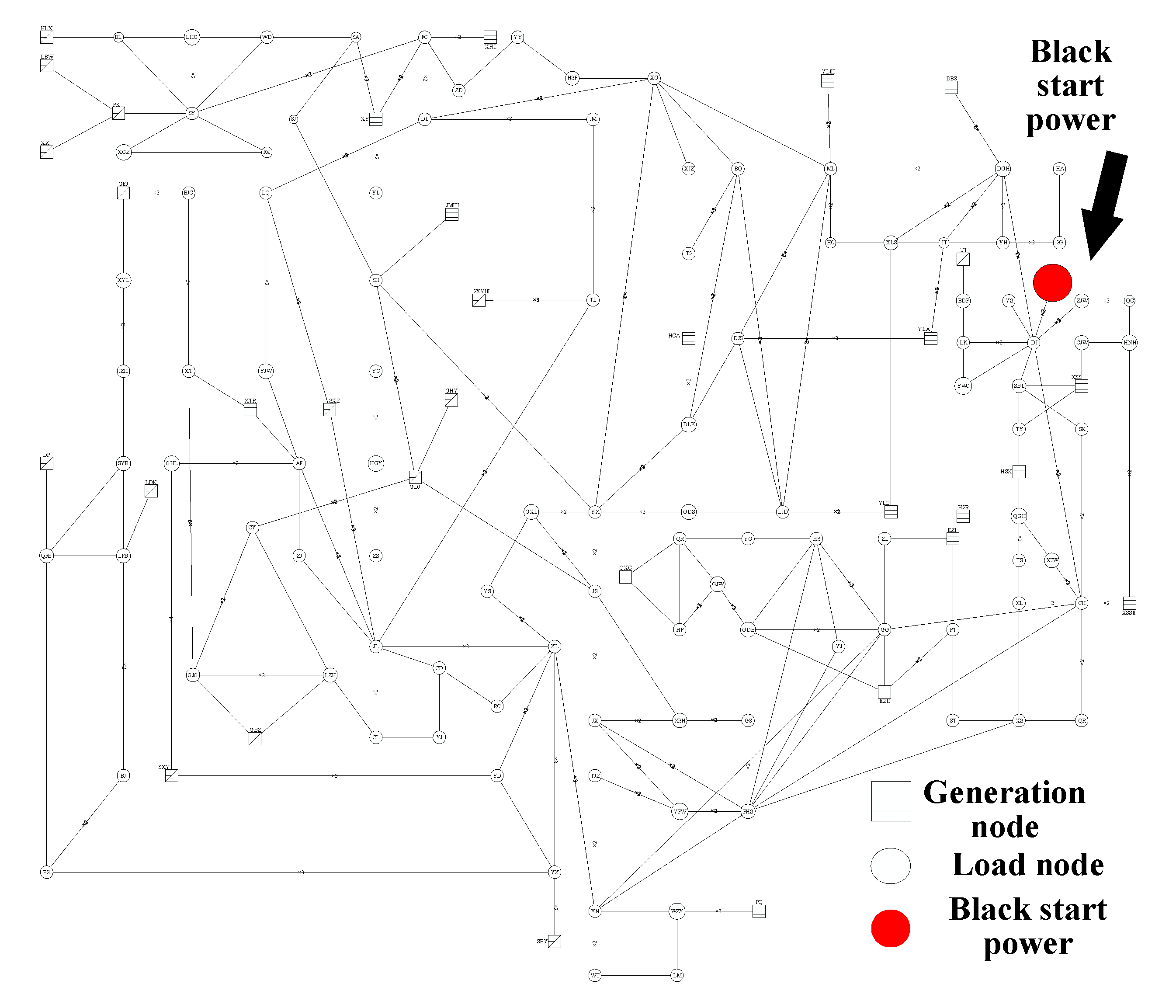
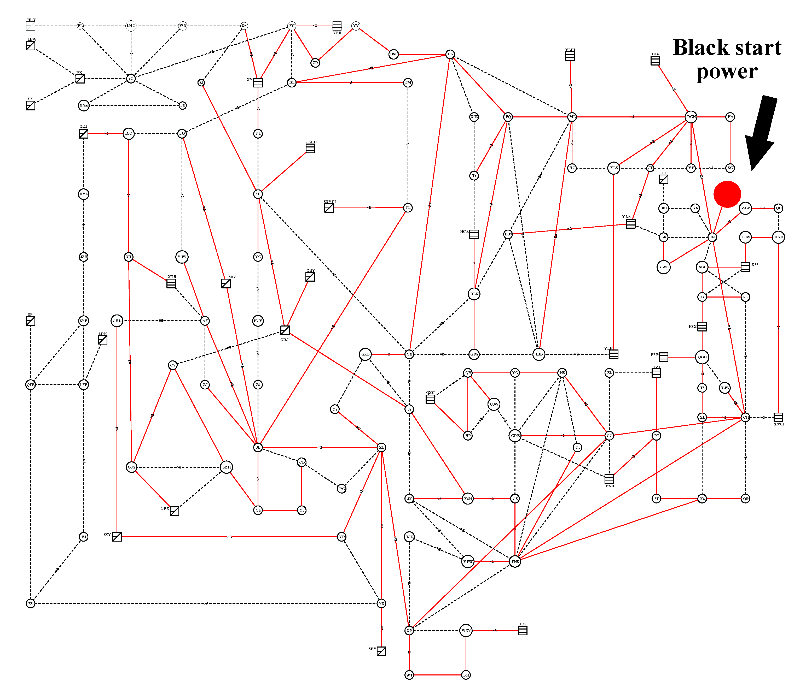
4.3. Analysis of an Actual Power Grid Calculation Example
5. Conclusions
- The proposed strategy can optimize the recovery path of grid units and load nodes. Considering the recovery success rate formed by the line and transformer parameters on the recovery path, it can effectively reduce the nodes involved in too many devices during recovery and reduce the risk of starting failure caused by inrush current or line overvoltage.
- When considering the restoration index in the outage scenario, the scheme in this paper can optimize the comprehensive effect of the recovery time and the recovery success rate of the grid structure. Considering the specific recovery process in the outage scenario, it can effectively reflect the difference of recovery ability between different grid structures and optimize the recovery ability of grid structures according to the recovery index.
- The proposed strategy can effectively adjust the optimal scheme with the change of equipment parameters and the position of the black start power supply.
Author Contributions
Funding
Acknowledgments
Conflicts of Interest
Nomenclature
| The Optimal Solution under Normal Power Supply Scenario | |
| the power supply capacity index, the safety margin index, transmission smoothness index | |
| the power saving rate, the important load saving rate | |
| the total number of generation nodes in the grid | |
| the rated generation capacity of the k-th generation node in the grid | |
| the total number of generation group nodes in the grid before optimization | |
| the rated generation capacity of the i-th generation node in the grid before optimization | |
| the total number of load nodes in the grid | |
| the power consumption of the k-th load node in the grid | |
| the weight of load nodes in the grid, which is selected based on the power user level, so as to distinguish the user importance level | |
| the total number of load nodes in the grid before optimization | |
| the rated power generation of the i-th power generation node in the grid before optimization | |
| the node voltage margin, the power margin of the generating node, the power margin weight of the generating node | |
| the total number of nodes in the grid, the weight of the k-th node in the grid | |
| the voltage margin of the k-th node | |
| the rated voltage of k-th node, the upper limit of the allowable voltage of the k-th node, the lower limit of the allowable voltage of the k-th node | |
| the maximum active power output of the i-th generation node in the grid structure. | |
| the number of reserved lines in the grid | |
| the weight of the k-th line in the grid, the active power transmission limit of the k-th line in the grid, the active power transmission of the k-th line in the grid in the normal power supply scenario | |
| Initialization of particle swarm | |
| the flight speed of particle i | |
| The optimal location of particle i | |
| the optimal location of particle swarm | |
| the learning factor | |
| random numbers in the [0,1] interval. | |
| the optimal solution in case of power failure | |
| the recovery index. | |
| the recovery success rate | |
| the total recovery time, the total recovery time weight | |
| the set of paths | |
| Line index, transformer index, the optimal recovery path of the generator set i to be recovered | |
| the equivalent capacitive reactance of the branch j in the path, the maximum capacitive reactance value of all lines | |
| the saturation flux of the transformer | |
| the time required to start the unit in the first step, the time required to recover the remaining nodes in the second step | |
| the charging time of the j-th line included in the path, the starting time of the k-th station included in the path, the starting time of the black start unit | |
| the equivalent length of line i | |
| the longest path between the unrecovered node and the recovered node | |
| the climbing rate of the k-th generation node, the output of the k-th generation node after system recovery |
Appendix A

| Bus Number | Pd | Qd | Vmax | Vmin | Load Importance Level |
|---|---|---|---|---|---|
| 1 | 0 | 0 | 1.05 | 0.95 | - |
| 2 | 21.7 | 12.7 | 1.1 | 0.95 | - |
| 3 | 2.4 | 1.2 | 1.05 | 0.95 | 2 |
| 4 | 7.6 | 1.6 | 1.05 | 0.95 | 1 |
| 5 | 0 | 0 | 1.05 | 0.95 | 3 |
| 6 | 0 | 0 | 1.05 | 0.95 | 3 |
| 7 | 22.8 | 10.9 | 1.05 | 0.95 | 1 |
| 8 | 30 | 30 | 1.05 | 0.95 | 1 |
| 9 | 0 | 0 | 1.05 | 0.95 | 3 |
| 10 | 5.8 | 2 | 1.05 | 0.95 | 2 |
| 11 | 0 | 0 | 1.05 | 0.95 | 3 |
| 12 | 11.2 | 7.5 | 1.05 | 0.95 | 2 |
| 13 | 0 | 0 | 1.05 | 0.95 | -- |
| 14 | 6.2 | 1.6 | 1.05 | 0.95 | 1 |
| 15 | 8.2 | 2.5 | 1.05 | 0.95 | 1 |
| 16 | 3.5 | 1.8 | 1.05 | 0.95 | 2 |
| 17 | 9 | 5.8 | 1.05 | 0.95 | 2 |
| 18 | 3.2 | 0.9 | 1.05 | 0.95 | 1 |
| 19 | 9.5 | 3.4 | 1.05 | 0.95 | 2 |
| 20 | 2.2 | 0.7 | 1.05 | 0.95 | 1 |
| 21 | 17.5 | 11.2 | 1.05 | 0.95 | 2 |
| 22 | 0 | 0 | 1.05 | 0.95 | -- |
| 23 | 3.2 | 1.6 | 1.05 | 0.95 | -- |
| 24 | 8.7 | 6.7 | 1.05 | 0.95 | 1 |
| 25 | 0 | 0 | 1.05 | 0.95 | 3 |
| 26 | 3.5 | 2.3 | 1.05 | 0.95 | 1 |
| 27 | 0 | 0 | 1.05 | 0.95 | -- |
| 28 | 0 | 0 | 1.05 | 0.95 | 3 |
| 29 | 2.4 | 0.9 | 1.05 | 0.95 | 1 |
| 30 | 10.6 | 1.9 | 1.05 | 0.95 | 2 |
| Bus Number | Maximum Output (MW) | Unit Capacity (MW) | Climbing Rate (MW/min) | Startup Time (min) |
|---|---|---|---|---|
| 1 | 80 | 100 | 10 | 30 |
| 2 | 80 | 100 | 10 | 25 |
| 22 | 50 | 100 | 8 | 30 |
| 27 | 55 | 100 | 8 | 30 |
| 23 | 30 | 100 | 3.5 | 25 |
| 13 | 40 | 100 | 5 | 25 |
| From Bus | To Bus | r | x | b | Allowable Capacity of Long-Distance Transmission Branch (MVA) | Charging Time (min) |
|---|---|---|---|---|---|---|
| 1 | 2 | 0.02 | 0.06 | 0.03 | 130 | 8 |
| 1 | 3 | 0.05 | 0.19 | 0.02 | 130 | 8 |
| 2 | 4 | 0.06 | 017 | 0.02 | 65 | 5 |
| 3 | 4 | 0.01 | 0.04 | 0 | 130 | 8 |
| 2 | 5 | 0.05 | 0.2 | 0.02 | 130 | 8 |
| 2 | 6 | 0.06 | 0.18 | 0.02 | 65 | 5 |
| 4 | 6 | 0.01 | 0.04 | 0 | 90 | 7 |
| 5 | 7 | 0.05 | 0.12 | 0.01 | 70 | 6 |
| 6 | 7 | 0.03 | 0.08 | 0.01 | 130 | 8 |
| 6 | 8 | 0.01 | 0.04 | 0 | 32 | 4 |
| 6 | 9 | 0 | 0.21 | 0 | 65 | 5 |
| 6 | 10 | 0 | 0.56 | 0 | 32 | 4 |
| 9 | 11 | 0 | 0.21 | 0 | 65 | 5 |
| 9 | 10 | 0 | 0.11 | 0 | 65 | 5 |
| 4 | 12 | 0 | 0.26 | 0 | 65 | 5 |
| 12 | 13 | 0 | 0.14 | 0 | 65 | 5 |
| 12 | 14 | 0.12 | 0.26 | 0 | 32 | 4 |
| 12 | 15 | 0.07 | 0.13 | 0 | 32 | 4 |
| 12 | 16 | 0.09 | 0.2 | 0 | 32 | 4 |
| 14 | 15 | 0.22 | 0.2 | 0 | 16 | 3 |
| 16 | 17 | 0.08 | 0.19 | 0 | 16 | 3 |
| 15 | 18 | 0.11 | 0.22 | 0 | 16 | 3 |
| 18 | 19 | 0.06 | 0.13 | 0 | 16 | 3 |
| 19 | 20 | 0.03 | 0.07 | 0 | 32 | 4 |
| 10 | 20 | 0.09 | 0.21 | 0 | 32 | 4 |
| 10 | 17 | 0.03 | 0.08 | 0 | 32 | 4 |
| 10 | 21 | 0.03 | 0.07 | 0 | 32 | 4 |
| 10 | 22 | 0.07 | 0.15 | 0 | 32 | 4 |
| 21 | 22 | 0.01 | 0.02 | 0 | 32 | 4 |
| 15 | 23 | 0.1 | 0.2 | 0 | 16 | 3 |
| 22 | 24 | 0.12 | 0.18 | 0 | 16 | 3 |
| 23 | 24 | 0.13 | 0.27 | 0 | 16 | 3 |
| 24 | 25 | 0.19 | 0.33 | 0 | 16 | 3 |
| 25 | 26 | 0.25 | 0.38 | 0 | 16 | 3 |
| 25 | 27 | 0.11 | 0.21 | 0 | 16 | 3 |
| 28 | 27 | 0 | 0.4 | 0 | 65 | 5 |
| 27 | 29 | 0.22 | 0.42 | 0 | 16 | 3 |
| 27 | 30 | 0.32 | 0.6 | 0 | 16 | 3 |
| 29 | 30 | 0.24 | 0.45 | 0 | 16 | 3 |
| 8 | 28 | 0.06 | 0.2 | 0.02 | 32 | 4 |
| 6 | 28 | 0.02 | 0.06 | 0.01 | 32 | 4 |
References
- Sun, H.D.; Xu, T.; Guo, Q.; Li, G.F. Analysis on Blackout in Great Britain Power Grid on August 9th, 2019 and its Enlightenment to Power Grid in China. Proc. CSEE 2019, 21, 1–11. [Google Scholar]
- Yi, J.; Bu, G.Q.; Guo, Q. Analysis of “3.21” blackout in Brazil and Its Enlightenment to China Power Grid. Power Syst. Autom. 2019, 43, 7–15. [Google Scholar]
- Lin, W.F.; Guo, Q.; Yi, J. Analysis on Blackout in Argentine Power Grid on June 16, 2019 and Its Enlightenment to Power Grid in China. Proc. CSEE 2020. [Google Scholar] [CrossRef]
- Mariani, E.; Mastroianni, F.; Romano, V. Field Experiences in Reenergization of Electrical Networks from Thermal and Hydro Units. IEEE Trans. Power Appar. Syst. 1984, PAS-103, 1707–1713. [Google Scholar] [CrossRef]
- Salvati, R.; Sforna, M.; Pozzi, M. Restoration project Italian power restoration plan. IEEE Power Energy Mag. 2004, 2, 44–51. [Google Scholar] [CrossRef]
- Liu, Y.T.; Wang, H.T.; Ye, H. chapter one. Theory and Technology of Power System Restoration; Science Press: Beijing, China, 2014; Volume 3, pp. 1–58. [Google Scholar]
- Zhang, S. Simulation Model and Risk Assessment of Power System Blackout; North China Electric Power University, Post-Graduate: Baoding, China, 2010. [Google Scholar]
- Gu, X.P.; Yang, C.; Liang, H.P.; Li, S.Y. Path Optimization of Power System Restoration With HVDC Transmission. Power Syst. Technol. 2019, 43, 2020–2032. [Google Scholar]
- Kun, J.T.; Shu, S.D.; Yu, Q.L. Asynchronous distributed global power flow method for transmission–distribution coordinated analysis considering communication conditions. Electr. Power Syst. Res. 2020, 182, 106256. [Google Scholar]
- Feng, S.; Yi, Z.; Gang, W. Study on charging and discharging characteristics of energy storage system in wind storage power plant under the condition of black start. Adv. Mater. Res. 2015, 1070, 443–448. [Google Scholar]
- Majid, E.M.; Hamid, F.; Mahdi, F. A Novel Method of Optimal Capacitor Placement in the Presence of Harmonics for Power Distribution Network Using NSGA-II Multi-Objective Genetic Optimization Algorithm. Sustainability 2020, 10, 2344. [Google Scholar]
- Damir, J.; Josip, V.; Petar, S. Optimal Reconfiguration of Distribution Networks Using Hybrid Heuristic-Genetic Algorithm. Sustainability 2020, 13, 1544. [Google Scholar]
- Pei, Z.; Yang, L.W.; Li, K.L. Short-Term Wind Power Prediction Using GA-BP Neural Network Based on DBSCAN Algorithm Outlier Identification. Sustainability 2020, 8, 157. [Google Scholar]
- El-Zonkoly; Amany, M. Renewable energy sources for complete optimal power system black-start restoration. IET Gener. Transm. Distrib. 2015, 9, 531–539. [Google Scholar] [CrossRef]
- Fei, L.P.; Jun, L.; Ben, D.T. Stacked-GRU Based Power System Transient Stability Assessment Method. Sustainability 2020, 11, 121. [Google Scholar]
- GU, M.H.; Sun, W.B.; Li, P.P. Evaluation Index System for Urban Elastic Distribution Network in the Face of Extreme Disturbance Events. Proc. CSU-EPSA 2018, 7, 103–109. [Google Scholar]
- Dong, F.F.; Liu, D.C.; Wu, J. A Method of Constructing Core Backbone Grid Based on Improved BBO Optimization Algorithm and Survivability of Power Grid. Proc. CSEE 2014, 34, 2659–2667. [Google Scholar]
- Zhu, H.N.; Liu, Y.T.; Qiu, X.Z. Optimal Restoration Unit Selection Considering Success Rate during Black StartStage. Autom. Electr. Power Syst. 2013, 22, 34–40. [Google Scholar]
- Feng, L.; Jin, L.M.; Zhang, T.Z. Optimal Restoration Unit Selection Considering Success Rate during Black StartStage. Proc. CSEE 2016, 36, 4904–4910. [Google Scholar]
- Zhao, Y.X.; Han, C.; Lin, Z.Z. Two-stage Core Backbone Network Optimization Strategy for Power Systems with Renewable Energy. Power Syst. Technol. 2019, 43, 16–31. [Google Scholar]
- Huan, J.J.; Wei, B.; Sui, Y. A Multi-Objective Planning Method of Urban Secure Power Networks Guaranteed Against Typhoon and Disaster. Power Syst. Technol. 2018, 15, 12–25. [Google Scholar]
- Zhou, Z.; Lei, L.; Wu, H.B. Study on Survivability Evaluation of Core Backbone Network Based on Multiple Indexes Synthesis Method. Smart Power 2018, 6, 1–6. [Google Scholar]
- Bi, T.Z.; Huang, S.F.; Xue, A.C. An Approach for Critical Lines Identification Based on the Survivability of Power Grid. Proc. CSEE 2011, 7, 31–37. [Google Scholar]
- Golshani, A.; Sun, W.; Zhou, Q. Incorporating wind energy in power system restoration planning. IEEE Transactions on Smart Grid 2019, 10, 16–28. [Google Scholar] [CrossRef]
- Fu, Z.H. Network Reconstruction and Partition Restoration Strategy in Power System Restoration; Zhejiang University, Post-Graduate: Hangzhou, China, 2017. [Google Scholar]
- Lin, X.; Liu, Y.; Xu, L.X. A method of searching backbone grid based on survivability of power system. Electr. Meas. Instrum. 2019, 12, 49–56. [Google Scholar]


| Option | Starting Unit | Optimal Path | Fable | T/min |
|---|---|---|---|---|
| 1 | 2 | 1-3-4-2 | 0.315 | 116 |
| 13 | 1-3-4-12-13 | |||
| 22 | 1-3-4-12-16-17-10-20-19-18-15-23-24-22 | |||
| 23 | 1-3-4-12-16-17-10-20-19-18-15-23 | |||
| 27 | 1-3-4-6-8-28-27 | |||
| 2 | 2 | 1-3-4-2 | 0.427 | 110 |
| 13 | 1-3-4-12-13 | |||
| 22 | 1-3-4-6-10-22 | |||
| 23 | 1-3-4-12-15-23 | |||
| 3 | 13 | 1-3-4-12-13 | 0.392 | 103 |
| 22 | 1-3-4-6-10-22 | |||
| 23 | 1-3-4-6-10-22-24-23 | |||
| 27 | 1-3-4-6-10-22-24-25-27 |
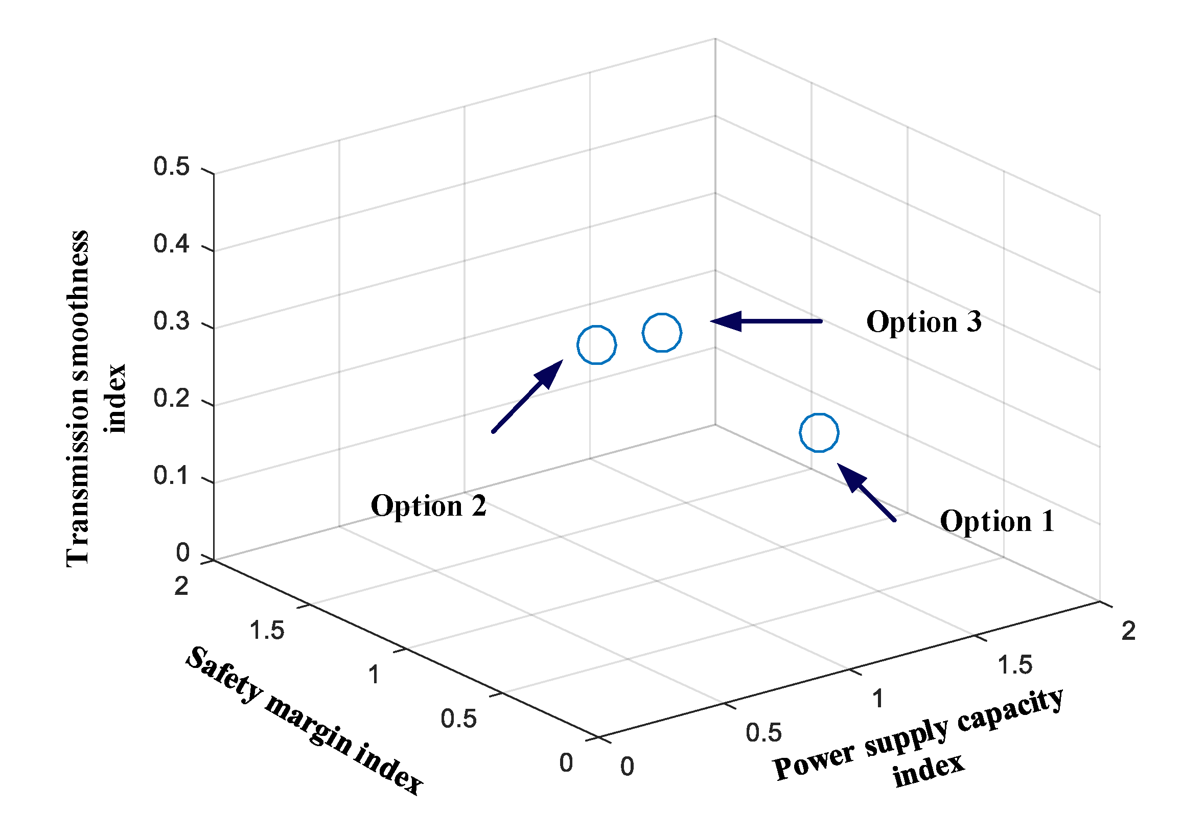
| Grid Construction Considerations | Alternative Program | f1 | f2 | f3 | frec | Optimal Scheme |
|---|---|---|---|---|---|---|
| Optimization in normal scenarios | 1 | 1.81 | 1.21 | 0.10 | - | Based on focus selection |
| 2 | 1.53 | 1.97 | 0.15 | - | ||
| 3 | 1.42 | 1.49 | 0.23 | - | ||
| Increase outage scenario optimization | 1 | 1.81 | 1.21 | 0.10 | 0.083 | Option 2 |
| 2 | 1.53 | 1.97 | 0.15 | 0.207 | ||
| 3 | 1.42 | 1.49 | 0.23 | 0.186 | ||
| Method in literature [26] | --- | 1.62 | 1.92 | 0.18 | 0.153 | Option 4 |
| Method in literature [22] | --- | 1.58 | 1.83 | 0.21 | 0.102 | Option 5 |
| Black Start Power Node | Alternative Option | Optimal Option | |
|---|---|---|---|
| 1 | 1 | 0.083 | Option 2 |
| 2 | 0.207 | ||
| 3 | 0.186 | ||
| 22 | 1 | 0.053 | Option 3 |
| 2 | 0.192 | ||
| 3 | 0.201 |
© 2020 by the authors. Licensee MDPI, Basel, Switzerland. This article is an open access article distributed under the terms and conditions of the Creative Commons Attribution (CC BY) license (http://creativecommons.org/licenses/by/4.0/).
Share and Cite
Zhang, S.; Zhao, J.; Weng, Y.; Liu, D.; Ma, W.; Ma, Y. Construction Method of a Guaranteed Grid Considering the Specific Recovery Process. Sustainability 2020, 12, 3935. https://doi.org/10.3390/su12093935
Zhang S, Zhao J, Weng Y, Liu D, Ma W, Ma Y. Construction Method of a Guaranteed Grid Considering the Specific Recovery Process. Sustainability. 2020; 12(9):3935. https://doi.org/10.3390/su12093935
Chicago/Turabian StyleZhang, Shengfeng, Jie Zhao, Yixuan Weng, Dichen Liu, Weizhe Ma, and Yuhui Ma. 2020. "Construction Method of a Guaranteed Grid Considering the Specific Recovery Process" Sustainability 12, no. 9: 3935. https://doi.org/10.3390/su12093935