Experimental Study Based on Game Theory on the Private, Voluntary Supply Mechanisms of Goods for Forestry Infrastructure from the Perspective of Quasi-Public Goods

Abstract

The existing research on forestry infrastructure has focused on suggestions from other areas of forestry research: that forestry infrastructure should be completed and improved. However, research on forestry infrastructure is relatively rare. In the real world, there are various problems with creating forestry infrastructure, such as complex approval procedures for facility construction, irrational facility layout, insufficient funding for facility construction, and conflicts between the nature of land used for facility construction and the nature of forest land. This paper uses game theory to analyze the behavior of forest infrastructure goods suppliers. Relevant parameters related to forest area infrastructure were designed, including communication, environmental certainty, information feedback, and reward and punishment mechanisms, and experimental economics methods were used to simulate accurate behavior regarding the supply of goods. Then, the key factors that affect the provision of quasi-public goods for forestry infrastructure were studied. At the end of the paper, some targeted suggestions that distinguish rural infrastructure from general infrastructure are given.

1. Introduction

Forestry infrastructure refers to engineering facilities for forestry public services that provide economic, social, and ecological benefits, such as paths for cycling, tool storerooms, and transfer facilities. Forestry infrastructure helps with the sustainable development of the forestry industry. Research on the private and voluntary supply of goods for forestry infrastructure is important to ensure long-term supplies. Sound forestry infrastructure can promote the sustainable development of forestry production.

Up to now, the research on forestry infrastructure supplies has mainly focused on analyses of, e.g., insufficient supplies, low quality, and a shortage of funds [1,2,3,4,5,6,7,8]. Some scholars have also studied forest roads. Road location and design is a complex engineering problem involving economic and environmental requirements [9]. For instance, Enache et al. [10] carried out research on how the extraction distance and correction factors can be computed and used for assessing forest road options in a more efficient and effective manner, utilizing process automation in geographic information systems. Hayati et al. [11] have considered skidding costs, road construction, maintenance costs, and harvesting volume to confirm the optimum forest road network density and evaluate the quantity and quality of existing forest road networks. Laschi et al. [12] have developed a decision support system to assist managers in the process of forest road network planning, exploiting multicriteria analyses, an analytic hierarchy process, and geographic information systems. Parsakhoo and Mostafa [13] have summarized the results of a road network analysis (RNA) and have evaluated the shortest path (to save travel time) in the city of Gorgan’s public road network in Iran. Picchio et al. [14] have tested accuracy in estimating areas accessible for winching along skid trails: they used three geographic information systems, namely the correct distance method (CDM), the real distance buffer method 12 (RDBM12), and the real distance buffer method 10 (RDBM10). However, research on forestry infrastructure supplies has not been sufficient.

Forestry infrastructure is getting more and more attention. Many studies have mentioned the importance of forestry infrastructure. In terms of forestry production activities, many scholars believe that a sound forestry infrastructure can promote the development of a forestry economy and enhance the forest tenure reform system (the forest tenure reform system distinguishes between forest ownership, forest use rights, and forest land use rights; its purpose is to analyze property rights clearly) and forest operations [5,15,16,17,18]. Gumus and Turk [19] have analyzed timber extraction by farm tractors, developing a new skid trail pattern design using linear programming (LP) and geographic information systems.

The development of an under-forest economy (an under-forest economy is based on the ecological environment of forest land, using forest land resources, and carrying out multiple forest and agricultural operations, animal husbandry, and other projects within a forest) and disaster prevention in forest areas are inexorably linked to a sound forestry infrastructure [20,21,22,23,24,25]. Sound forestry infrastructure is not only conducive to accelerating the circulation of forest products, but also can improve the efficiency of the use of forestry industry information resources [26,27]. In terms of environmental protection, one study has shown that the more extreme climatic changes are, the more infrastructure support is required [28]. As for environmental planning, some scholars believe that a sound forestry infrastructure is integral to ecological restoration after a disaster [29,30]. Therefore, many scholars have suggested that infrastructure construction and investment should be strengthened to improve forestry foundation facilities [5,31,32].

Forestry infrastructure is a part of “general goods”, which can be divided into private goods, club goods, crowded goods, or pure public goods according to a four-point method. Of these, club goods and crowded goods can also be called quasi-public goods. In reality, the supply of quasi-public goods comes from diverse sources, and problems with adequate supply are common. Therefore, an ample supply of quasi-public goods can greatly improve economic outcomes. There have been many studies on the supply of quasi-public goods. In terms of research on the effective supply of quasi-public goods, most scholars have written that the private supply of quasi-public goods is more efficient than a government supply alone [33,34,35,36]. In terms of methods for supplying quasi-public goods, scholars have written that except for the government’s supply, individuals, enterprises, and organizations should also be involved [37,38]. This paper studies supply mechanisms for goods for forestry infrastructure from the perspective of quasi-public goods.

In terms of research on the supply of quasi-public goods, most scholars have used game theory [39,40,41,42,43]. They have shown that it is feasible to analyze the supply mechanism of quasi-public goods utilizing game theory. This paper draws on existing research and uses game theory to analyze the supply mechanisms of quasi-public goods for forestry infrastructure. Most papers on the supply of quasi-public goods, on the contrary, have been limited to a theoretical level and have lacked empirical research.

One of the main focuses of experimental economics methods is the study of public goods [44]. With regard to experiments on the supply of quasi-public goods, some scholars have found that environmental uncertainty will affect the level of cooperation [45]. Jane and Rick [46] have studied the impact of information feedback on cooperation, indicating that information feedback can promote the supply of public goods. However, Weimann [47] and Croson [48] did not find a role for information feedback in their experiment. Some scholars have studied the impact of information feedback methods on the supply of public goods [49,50,51,52]. In addition, other scholars have applied punishment mechanisms to the study of the impact of information feedback on the supply of public goods [53,54]. Traditional methods of data collection have generally included literature surveys and questionnaires, which can lead to static data and may only represent a single moment in time. Experimental economic methods are solutions to these problems. Therefore, this paper uses experimental economics methods to verify the results of a game theory analysis. We selected four control variables for the experiments. Using the above-mentioned research, we combined the characteristics of the supply of goods for forestry infrastructure: communication, information feedback, environment determination, and reward and punishment mechanisms.

To sum up, this paper uses game theory to study the supply mechanisms of quasi-public goods for forestry infrastructure and then uses experimental economics to verify the theoretical results. Using game theory analysis, we include noncooperative games and cooperative games, and determine a game payment matrix according to the current situation of forestry production. In the empirical research section, we use experimental economics, selecting four control variables: whether to communicate, whether the environment is determined, whether the information is feedback information, and whether there is a reward and punishment mechanism. The research object is quasi-public goods for forestry infrastructure, where we simulate the supply process of quasi-public goods for forestry infrastructure. Finally, we verify the main factors that affect cooperative games.

2. Materials and Methods

2.1. Game Theory Analysis

Game theory is a mathematical theory and method for studying the phenomena of struggle or competition. The basic concepts include people, actions, information, strategies, benefits, equilibrium, and results. These can be divided into different categories according to different classification methods. Among them, there are noncooperative games and cooperative games (depending on the relationship between individual interests and collective interests) [55,56]. Using this game classification, we first studied the noncooperative game equilibrium results, and then studied the cooperative game equilibrium results. In conclusion, the cooperative game equilibrium results were better than the results from the noncooperative games. A detailed analysis follows.

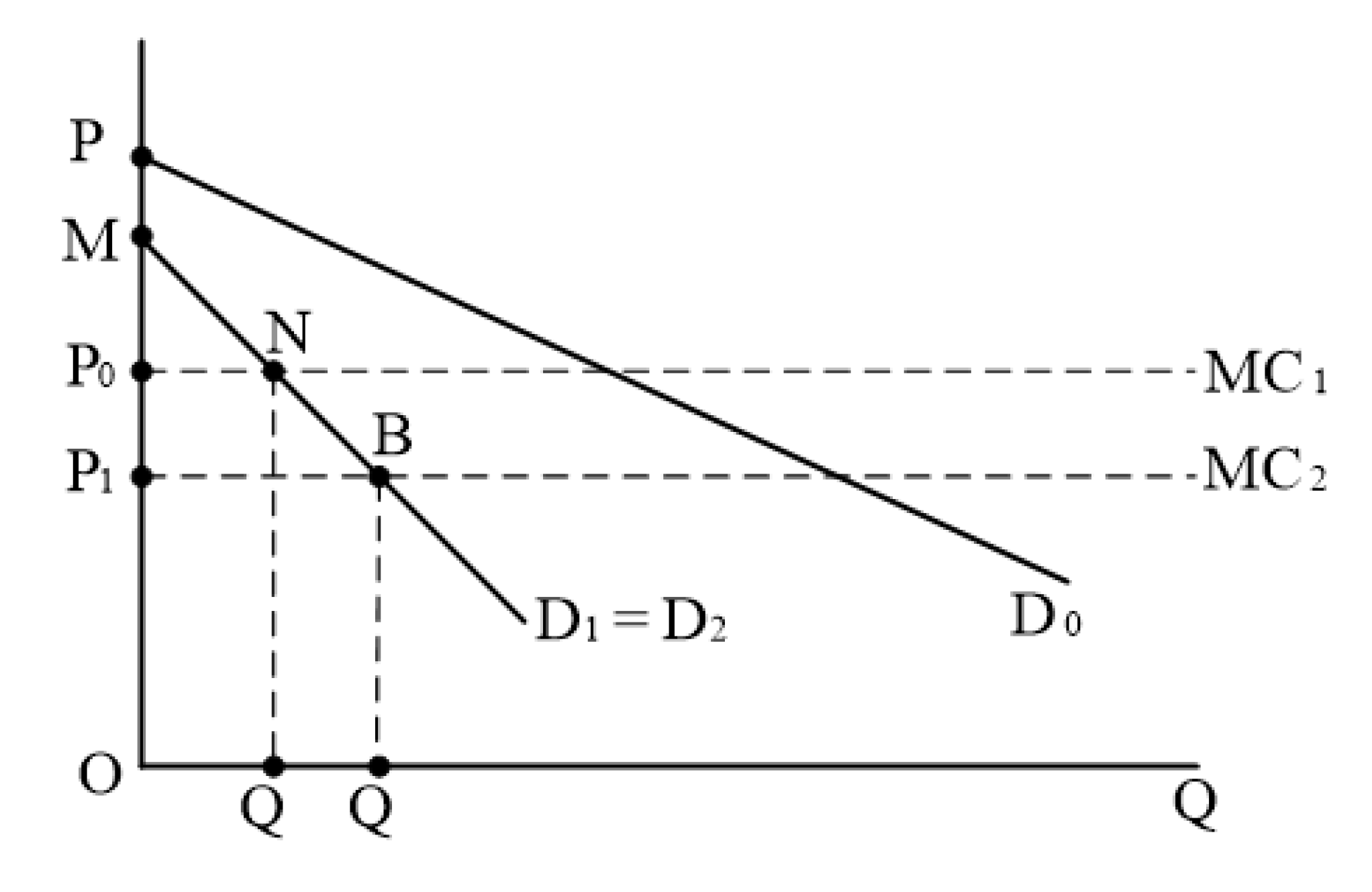
2.1.1. Noncooperative Games

Noncooperative game theory can be defined as game theory with complete rules. Thus, it can be described with three features. First, the rules are complete. Second, the ultimate decision units are the individual players. Third, commitments are not available, unless allowed for by the rules of the game [56].

• Forestry Infrastructure Is Not Provided When Income Is the Same

Suppose there are two rational people in a forest area, subject A and subject B, with the same income. Due to the difference in the quantity of forest land resources owned by forest farmers and the different requirements for forestry infrastructure, different forest farmers also receive different benefits from quasi-public goods for forestry infrastructure. When these two people cooperate to provide goods, the cost of each person’s burden varies according to the degree of demand. Those with a high demand have a higher cost, and those with low demand have lower costs. Suppose subject A has a large quantity of forest land resources and a high demand for quasi-public goods for forestry infrastructure. The benefit of providing forestry infrastructure is R1, and the cost of the burden is C1. Subject B has a small quantity of forest land resources and has a low demand for public-goods-based forestry infrastructure. The benefit of providing forestry infrastructure is R2, and the cost of the burden is C2. The cost of forestry infrastructure construction is 2C, of which C1 + C2 = 2C. If both of them refuse to provide goods, the return is 0 [57]. The payment matrix is shown in

Table 1. Payment matrix when income is the same.

	Subject B	Offers	Does Not Offer
Subject A
Offers		R1−C1, R2−C2	R1−2C, R2
Does not offer		R1, R2−2C	0, 0

.

The prisoner’s dilemma game is a standard example of a game that is analyzed in game theory that shows why two completely rational individuals might not cooperate, even if it appears that it is in their best interests to do so. Two members of a criminal gang are arrested and imprisoned. Each prisoner is in solitary confinement with no means of communicating with the other. The prosecutors lack sufficient evidence to convict the pair on the principal charge, but they have enough to convict both on a lesser charge. Simultaneously, the prosecutors offer each prisoner a bargain. Each prisoner is given the opportunity either to betray the other by testifying that the other committed the crime, or to cooperate with the other by remaining silent. Here, when 2C > R1 > 0 and 2C > R2 > 0, the game is a prisoner’s dilemma game, and the Nash equilibrium is (not provide, not provide). The reason is that the construction costs of some quasi-public goods for forestry infrastructure are relatively high, but an individual’s income from forestry infrastructure is very low. If individuals provide money alone, the fund can run a deficit. At that time, rational participants will choose not to provide. (Not provide, not provide) is the Nash equilibrium, because not providing is the optimal strategy for everyone. No one has the motivation to change his/her strategy. A private, voluntary supply of forestry infrastructure will thus not exist [57].

The chicken game, also known as the hawk–dove game or the snowdrift game, is a game theory model of conflict for two players. The principle of the game is that while the outcome is ideal for one player to yield (to avoid the worst outcome if neither yields), individuals try to avoid this out of pride, not wanting to look like a “chicken”. Thus, each player taunts the other to increase the shame in yielding. However, when one player yields, the conflict is avoided, and the game is for the most part over. Here, when R1 > 2C > 0 and R2 > 2C > 0, the game is a chicken game, and the Nash equilibrium is (provide, not provide) and (not provide, provide). In this scenario, according to a rational person’s assumptions, each forest farmer wants to benefit from the actions of the others (hitchhiking). As both enjoy the same income, neither has the incentive to choose or provide first. At this time, the game is also deadlocked, and the private, voluntary supply of forestry infrastructure will not exist [57].

In summary, when two rational people in a forest area share the same income, if they do not choose to cooperate, they will not voluntarily provide goods for forest infrastructure.

• An Insufficient Supply of Forestry Infrastructure with Different Incomes

Suppose there is forest farmer A and forest farmer B in the same forest area. They have different incomes. Forest farmer A has a high income and forest farmer B has a low income. Each of them has two strategies for providing forestry infrastructure: providing or not providing.

Because high-income people usually provide forestry infrastructure in pursuit of some social benefit, such as reputation or fame, and low-income people only hope to meet their production needs, high-income earners benefit more from forestry infrastructure construction. In addition, high-income earners have enough money to provide goods for forestry infrastructure, but low-income earners do not. From the perspective of opportunity costs, the opportunity cost of providing forestry infrastructure is far lower for high-income earners.

Suppose the cost of building forestry infrastructure is 2C. In this scenario, both forest farmers choose to provide, the income of high-income earners is R1, and the cost is C1. The income of low-income earners is R2, and the cost is C2. At this point, R1 and R2 represent economic benefits, or basic production needs. When the high-income individual chooses to provide and the low-income individual chooses not to provide, the high-income individual earns R11, the cost is 2C, and the low-income individual earns R2. At this time, R11 is the sum of the economic benefits and social benefits of the high-income individual who provides forestry infrastructure, so R11 > R1. When the high-income individual chooses not to provide, and the low-income individual chooses to provide, the income of the high-income individual is R1, and the income of the low-income individual is R2. Because the opportunity cost of providing forestry infrastructure is higher for low-income individuals, the total cost is (2C + C0). When neither the high-income individual nor the low-income individual provide, their benefits are zero, and R1 > R2, R2 < (2C + C0), R11 > R1 > 2C. This situation is a typical rational pigs’ scenario [57]. With rational pigs, there are two pigs in a pigsty, a big pig and a small pig. The pigsty has a pedal on one side. When a pig steps on the pedal, a small amount of food will fall into the feeding tray on the other side of the pigsty, away from the pedal. When one pig steps on the pedal, the other pig has a chance to eat the food first. When a small pig steps on the pedal, the big pig will eat all the food before the small pig steps on the pedal and then runs to the feeding tray. When a big pig steps on the pedal, the small pig cannot eat all the food before the big pig steps on the pedal and then runs to the feeding tray. The specific payment matrix is shown in

Table 2. Rational pigs.

	Subject B	Offers	Does Not Offer
Subject A
Offers		R1−C1, R2−C2	R11−2C, R2
Does not offer		R1, R2−(2C + C0)	0, 0

.

In Table 2, subject A represents a high-income earner and subject B represents a low-income earner. The Nash equilibrium of this game is (provide, not provide), i.e., the high-income earner pays for the forestry infrastructure, and the low-income earner hitchhikes. This happens because the high-income earner does not mind letting the low-income earner hitchhike, and forestry infrastructure is provided. The high-income earner does not mind paying more, even if he/she bears the full cost.

2.1.2. Cooperative Games

Since rules are only broadly defined, the individual decision problems of players cannot be directly analyzed. Cooperative game theory avoids these difficulties by emphasizing coalitions of players. The study of coalitions implicitly assumes that such coalitions contain a presumption that players commit themselves, either by explicitly signing enforceable contracts or by transferring their decision-making powers. Hence, cooperative game theory is characterized by three features. First, rules are kept implicit. Second, the emphasis is on coalitions. Third, commitments are available [56].

• A Feasibility Analysis of Cooperative Games

When forest farmers cooperate to supply forestry infrastructure, the costs borne by individual forest farmers must be reduced, regardless of whether forest farmers have the same demand for forestry infrastructure. At this point, for a single forest farmer, consumer surplus will increase. The supply of forestry infrastructure increases for the entire forest area, achieving Pareto optimality. Assuming that forest farmers have the same demand for forestry infrastructure, a supply–demand model can be used to study the feasibility of a cooperative supply of goods for forestry infrastructure [57]. The specific analysis is shown in Figure 1.

In Figure 1, D₁ and D₂ represent the demand curve for forestry infrastructure for forest farmer A and forest farmer B, respectively. Because the demand for forestry infrastructure is the same, the two-day demand curves overlap. MC₁ indicates the cost when forest farmers provide forestry infrastructure separately. MC₂ indicates the supply cost borne by individual forest farmers when they cooperate with each other. Cooperation reduces the supply cost of individual forest farmers, so MC₂ < MC₁. It can be seen from Figure 1 that after cooperation, the supply of goods for forestry infrastructure increases from Q₀ to Q₁, and consumer surplus increases from S_△MNP0 to S_△MBP1. Through cooperation, the consumer surplus of individual forest farmers increases, and the supply of goods for forestry infrastructure is closer to the collective optimal quantity, achieving Pareto optimality.

• Conditions for Realizing a Cooperative Game of Private, Voluntary Supply

The “club” size of community: The “club” size of community must meet two conditions. One is that the “club” will exist steadily for a period of time to ensure that members of the community can repeat the game, and the other is that reward and punishment mechanisms can be implemented within the “club” to restrict free rides by community members. Medium-sized rural villages meet the above-mentioned “club” conditions [57].

When the game is repeated, members of medium-sized rural areas are relatively stable, and they are more familiar with each other and can monitor each other. Because this is a repeated game, participants in the community not only consider the benefits that can be obtained at the current stage, but also comprehensively consider the benefits that can be obtained in the next game, as well as the costs they are going to face. Therefore, the strategic choice over repeated games and the strategic choice during one game are different. At the same time, under the constraints of reward and punishment mechanisms, members of the community are more likely to choose cooperation strategies [57].

In the collection of quasi-public goods for forestry infrastructure in medium-sized rural areas, the members are relatively stable and can repeat the game [57]. Therefore, quasi-public goods for forestry infrastructure can be provided cooperatively in medium-sized rural areas.

2.2. Experimental Design

In order to study the main factors that affect cooperative games, this paper uses experimental economics methods. On the basis of the literature and real-life situations, four control variables were selected: whether there was communication, whether the environment was determined [58], whether the information was feedback information [58], and whether there was a reward and punishment mechanism [59]. A total of 12 experiments were designed, including 6 experiments in the nonexchange group and 6 experiments in the exchange group. The specific experimental design is shown in

Table 3. Specific design of private cooperative supply experiments.

Group Members Could Not Communicate	Group Members Could Communicate
Experiment 1 (NC): NF × U (10 rounds)	Experiment 1 (C): NF × U (10 rounds)
Experiment 2 (NC): NF × NU (10 rounds)	Experiment 2 (C): NF × NU (10 rounds)
Experiment 3 (NC): F × U × NP (10 rounds)	Experiment 3 (C): F × U × NP (10 rounds)
Experiment 4 (NC): F × U × P (10 rounds)	Experiment 4 (C): F × U × P (10 rounds)
Experiment 5 (NC): F × NU × NP (10 rounds)	Experiment 5 (C): F × NU × NP (10 rounds)
Experiment 6 (NC): F × NU × P (10 rounds)	Experiment 6 (C): F × NU × P (10 rounds)

Note: NC indicates that players could not communicate with each other, and C indicates that they could communicate with each other; F indicates that there was information feedback, and NF indicates that there was no information feedback; U indicates that the environment was determined, and NU indicates that the environment was uncertain; P indicates that there were reward and punishment measures, and NP indicates that there were no reward and punishment measures.

. The realization of the experimental design relied on Z-Tree software. This paper only shows a part of the experimental process and experimental procedures. For related information, see Appendix A.

2.2.1. Experimental Design Ideas

A voluntary donation mechanism was used to design the experiments. A total of n subjects were divided into m groups, and each group of (n/m) individuals played 10 rounds of games. Before the start of each round, everyone had an initial fund of e. They could choose to keep the funds in their own private accounts or to invest the funds in a public project. The funds could not be carried into the next round. If a member’s fund in the private account in round t was x_it (0 ≤ x_it ≤ e), and the investment amount in the public project was g_it (0 ≤ g_it ≤ e; x_it + g_it = e), then the public project’s total investment was G_t = ∑g_it in round t. Assume that the return on investment in a public project is β_t (0 ≤ β_t <1). When there is no environmental uncertainty, β₁ = β₂ = …… = β_T = β. When “environmental uncertainty” exists, β_t will be an independent and identically distributed random variable. If the distribution is set to a uniform distribution, that is, β_t ∈ [β, $\stackrel{—}{\beta }$], and the expected β_t (Eβ_t) is β, that is, Eβ_t = β, then the gain i in round t is as follows: п = x_it + β_tG_t = e − g_it + β_t∑g_it [58].

Four variables were selected: whether the group members could communicate, whether the information was feedback information, whether the environment was determined, and whether there was a reward and punishment mechanism. A total of 12 experiments were conducted. The specific experimental arrangement is shown in Table 3 below.

In each experiment, the group members were partners, that is, during the 10 rounds of experiments, the members of each group were fixed.

In the experiments in which members could communicate with each other, at the beginning of each experiment, the group members could discuss how to invest and decide how much to donate.

In the experiments with information feedback, after the end of each period, each group member was given the investment amount and investment income of others, in addition to his/her own investment amount, investment income, and β-value from that round. In the experiment without information feedback, after the end of each round of experiments, each group member only knew his/her own investment amount and investment income for the round.

In the experiments with a certain environment, at the beginning of each experiment, the group members knew the return rate β of the public account, which was relatively stable in reality. With environmental uncertainty, the investors did not know the return rate β before the start of each round of experiments, when they needed to estimate the return rate β and then decide how much to invest based on the estimated value of β. After the end of each round of experiments, they re-estimated the return rate β according to their own returns from the previous round and the influence of the social environment.

Rewards and punishments only existed in the experiments with information feedback. In the experiments with rewards and punishments, after each round of experiments, each group member in the group could decide to reward or punish the other members in accordance with the feedback information. After the information feedback was over and before the next round of experiments began, everyone in the group received 10 additional chips and had the opportunity to reward or punish others (note: they could not punish or reward themselves). When a person was rewarded or punished with one chip, the person’s gain increased or decreased by three chips. The maximum number of chips that each person could use for each target member was 5, which meant that each member could increase or decrease the profit of a target member by 15 at most [59].

2.2.2. Choice of Experimental Subjects

Experimental economics uses real people in society as experimental objects. In order to ensure the scientific nature of experimental economics, the selected subjects only have small differences or have differences that have nothing to do with or have little influence on the purpose of the experiment. Undergraduates and graduate students were chosen as candidates because of their relatively simple living environments, their relatively few differences, and their relatively strong ability to learn and understand. Moreover, using undergraduate and graduate students in economic experiments that require little or no practical experience can lead to better and more realistic effects. The recruitment of subjects was voluntary. Recruitment information that included the purpose and requirements of the experiment and the possible benefits and costs of participating in the experiment were also released to the public [60].

2.2.3. Statistical Analyses

The statistical analyses of the personal characteristics of the experimental subjects are shown in

Table 4. Statistical analyses of experimental objects.

Variables	Mean	Standard Deviation	Min	Median	Max
Gender	0.100	0.300	0.000	0.000	1.000
Ethnic group	0.950	0.218	0.000	1.000	1.000
Communist or not	0.050	0.218	0.000	0.000	1.000
Has taken out a loan or not	0.200	0.400	0.000	0.000	1.000
Part-time or not	0.500	0.500	0.000	0.500	1.000
Participated in the experiment or not	0.150	0.357	0.000	0.000	1.000
Average household income per month	3.250	0.829	1.000	3.000	4.000
Evaluation of self-reliability	3.800	0.600	2.000	4.000	5.000
Evaluation of stranger’s credibility	2.700	0.781	1.000	3.000	4.000

Note: gender (0 = female; 1 = male); ethnic group (0 = ethnic minority; 1 = ethnic Han); communist or not (0 = no; 1 = yes); Has taken out a loan or not (0 = no; 1 = yes); part-time or not (0 = no; 1 = yes); participated in the experiment or not (0 = no; 1 = yes); average household income per month (1 = 0–3000 RMB; 2 = 3001–6000 RMB; 3 = 6001–9000 RMB; 4 = 9000 RMB or more); evaluation of self-reliability(5 = very trustworthy; 4 = trustworthy; 3 = fair; 2 = untrustworthy; 1 = quite untrustworthy); evaluation of stranger’s credibility (5 = very trusting; 4 = trusting; 3 = fair; 2 = untrusting; 1 = quite untrusting).

. Variables such as gender, age, income, and trustworthiness of the experimental subjects were counted.

2.3. Methods

2.3.1. Mann–Whitney U Test

The Mann–Whitney U test, also called the “Mann–Whitney rank sum test”, was proposed by Mann and Whitney in 1947. The purpose was to test whether the means of two samples were significantly different. We used this method to analyze whether the experimental results of these two groups of experiments were different when a certain experimental variable changed. When the P value was less than 0.05, this indicated that the means of the two independent samples were significantly different.

2.3.2. Wilcoxon Signed-Rank Test

The Wilcoxon signed-rank test, or Wilcoxon symbol test, was proposed by Wilcoxon (F. Wilcoxon) in 1945. We used this method to test whether the differences between two types of data in the same group were significant. For example, a Wilcoxon signed-rank test was used to test whether the difference between “average donations after consultation” and “the average of actual donations” was significant (in experiment 1, with communication). When the P value was less than 0.05, this indicated that the means of the two independent samples were significantly different.

2.3.3. Multiple Regression Analysis

We used multiple regression to analyze the main factors that affect donations under different experimental conditions.

When P was less than 0.05, H0 could be rejected (there was no relationship between the two variables). Therefore, the P-value of the variable was less than 0.05, which indicated the explanatory variable had a significant effect on the dependent variable. Here, * means significant at the 0.05 probability level, and ** means significant at the 0.01 probability level.

3. Results

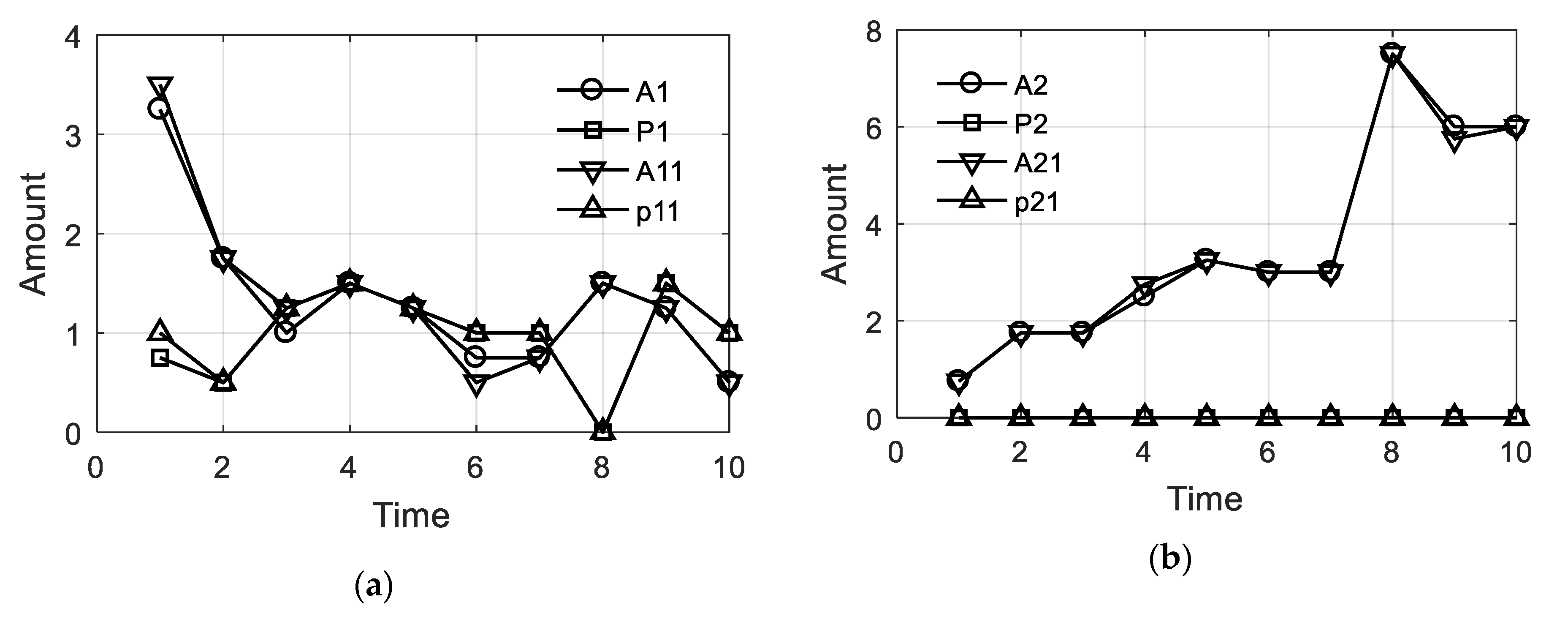
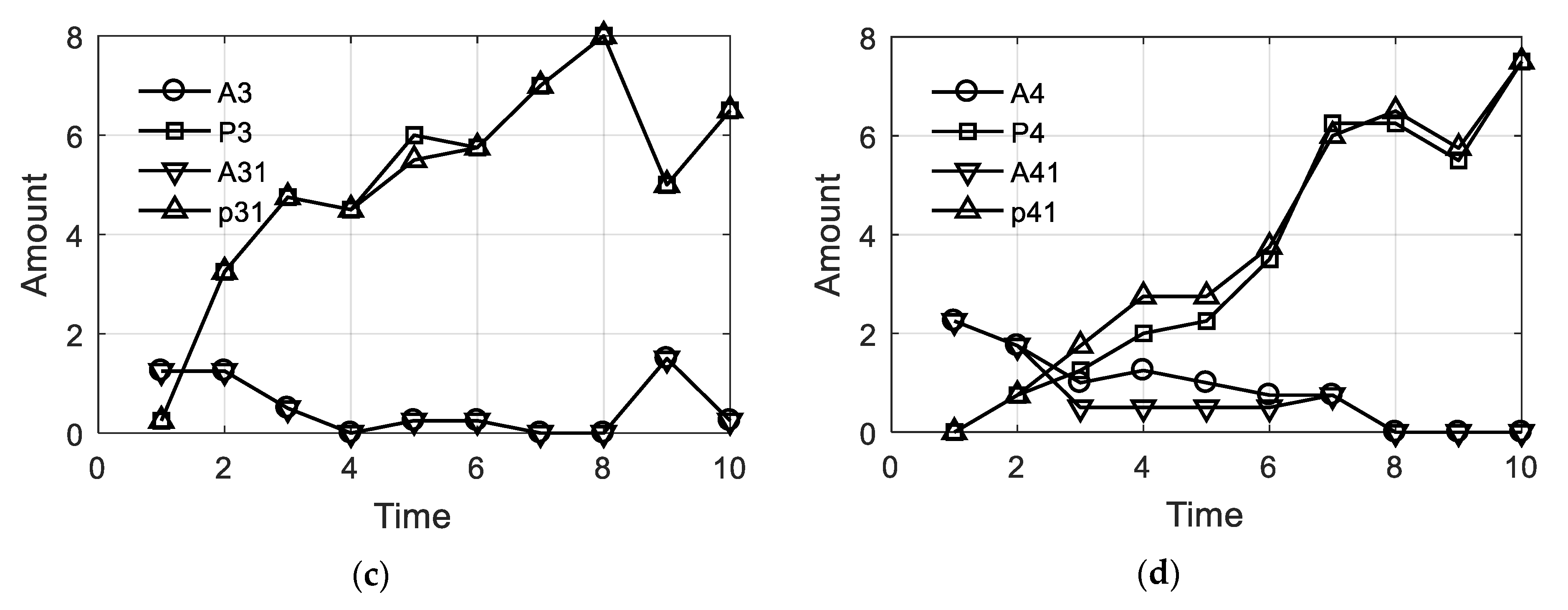
3.1. Statistical Analyses of Donation Amounts and Income under Different Experimental Conditions

In this paper, the donation amounts from the 12 groups of experiments were calculated using the mean, standard deviation, minimum value, median value, and maximum value. Basic statistical information on donation amounts from the different experiments is shown in

Table 5. Statistics of donation amounts under different experimental conditions.

Experiments	Variable	Mean	Standard Deviation	Min	Median	Max
Experiment 1 (NC) (10 rounds)	C1	2.520	2.106	0.000	2.000	7.200
Experiment 2 (NC) (10 rounds)	C2	6.275	4.483	0.000	6.000	20.000
Experiment 3 (NC) (10 rounds)	C3	3.800	1.646	0.000	4.000	6.000
Experiment 4 (NC) (10 rounds)	C4	14.925	3.085	5.000	15.000	20.000
Experiment 5 (NC) (10 rounds)	C5	4.790	1.934	1.000	5.000	10.000
Experiment 6 (NC) (10 rounds)	C6	13.125	3.116	5.000	13.500	20.000
Experiment 1 (C) (10 rounds)	C11	7.300	6.604	0.000	4.800	20.000
Experiment 2 (C) (10 rounds)	C22	5.975	6.207	0.000	5.000	20.000
Experiment 3 (C) (10 rounds)	C33	7.975	6.191	0.000	10.000	20.000
Experiment 4 (C) (10 rounds)	C44	14.675	2.611	9.000	15.000	20.000
Experiment 5 (C) (10 rounds)	C55	5.160	1.960	1.000	5.000	10.000
Experiment 6 (C) (10 rounds)	C66	10.075	4.424	5.000	8.500	20.000

Note: NC indicates that players could not communicate with each other, and C indicates that they could communicate with each other; F indicates that there was information feedback, and NF indicates that there was no information feedback; U indicates that the environment was determined, and NU indicates that the environment was uncertain; P indicates that there were reward and punishment measures, and NP that there were no reward and punishment measures. C1, C2, C3, C4, C5, C6, C11, C22, C33, C44, C55, and C66 represent the number of experimental coins donated under different experimental conditions. Before each round of experiments began, each member had 50 initial coins.

.

It is shown in Table 4 that the averages of Experiments 4 and 6 were the highest, and the average value of the communication group was higher than that of the noncommunication group, which shows that communication as well as reward and punishment mechanisms could improve the donation level as a whole.

Figure 2 shows the key factors affecting the supply of goods for forestry infrastructure, summarizing the results of five variables out of the six groups of experiments for comparative analyses: the “mean value of donations without communication”, “mean value of donations with communication”, “mean value of planned donations after communication”, “mean value of earnings without communication”, and “mean value of earnings with communication”. In Figure 2, C11, C21, C31, C41, C51, and C61 represent the “mean values of donations without communication”; C12, C22, C32, C42, C52, and C62 represent the “mean values of donations with communication”; C13, C23, C33, C43, C53, and C6 represent the “mean values of planned investment after communication”; R11, R21, R31, R41, R51, and R61 represent the “ mean values of earnings without communication”; and R12, R22, R32, R42, R52, R62 represent the “mean values of earnings with communication”.

The analysis of Figure 2 is as follows. Donations in Experiment 2 (C & NC) were slightly higher than in Experiment 1 (C & NC), which indicated that an uncertain environment could increase the donation level when there was no information feedback. However, the fluctuation in Experiment 2 (C & NC) was relatively large because of the uncertain environment. Experiment 3 (C & NC) had higher values, while Experiment 5 (C & NC) had greater fluctuations due to the uncertainty of the environment, indicating that when there was information feedback, a certain environment could improve the donation amounts. As for Experiment 4 and Experiment 6 (C & NC), Experiment 4 (C & NC) had slightly higher values than did Experiment 6 (C & NC), but the overall donation levels of Experiment 4 (C & NC) and Experiment 6 (C & NC) were higher than in the other experimental groups. In addition, Experiment 6 (C & NC) had large fluctuations due to the uncertain environment, which shows that a reward and punishment mechanism could improve the level of donations.

3.2. Impact of Communication on Donations

3.2.1. An Analysis of Hitchhiking Using Different Experimental Mechanisms

In order to study the free-riding situation due to different experimental mechanisms, a Wilcoxon signed-rank test was performed for “donations determined after consultation” and “actual donations” for the six groups of experiments.

Table 6. Wilcoxon signed-rank test results of the mean values of donations determined after consultation and actual donations in the experimental groups that were allowed to communicate.

Groups	Median of the Average of Donations after Consultation	Median of the Average of Actual Donations	Median Difference	P-Values
Experiment 1 (C)	4.600	5.050	−0.133	0.674
Experiment 2 (C)	8.375	4.083	2.875	0.012
Experiment 3 (C)	15.375	7.750	5.667	0.007
Experiment 4 (C)	15.4375	14.5833	0.7500	0.021
Experiment 5 (C)	5.500	5.308	0.125	0.192
Experiment 6 (C)	8.750	8.750	−0.200	0.207

indicates the results of a Wilcoxon signed-rank test that was used to check whether there was a difference between “donations determined after consultation” and “actual donations” in the six groups of experiments. The “median of the average of donations after consultation” and the “median of the average of actual donations” were calculated. “Median difference” refers to the median difference between “donations determined after consultation” and “actual donations”, and the “P-value” represents the significance level of the difference. When the P-value was less than 0.05, the difference was significant.

Table 6 shows the results when there was a reward and punishment mechanism (Experiment 4 (C) and Experiment 6 (C)). The actual and negotiated results of Experiment 4 (C) were significantly different, but those of Experiment 6 (C) were not significant. This shows that with a reward and punishment mechanism and a certain environment, the actual result was lower than the negotiated result. When the environment was uncertain, the actual and negotiated results were basically the same. The reason is that when the environment was determined, members could reasonably estimate their costs and benefits, and the actual donation amount was slightly lower than the negotiated result (but matched their needs). The P-value of Experiment 2 (C) was less than 0.05, which indicates that the difference in Experiment 2 (C) between the average value of the actual donation amount and the average value of the donation amount determined after consultation was significant. However, the P-value of Experiment 1 (C) was not significant. This shows that members were more likely to choose free-riding when there was no information feedback and the environment was uncertain. The difference between the average value of the actual donation amount and the average value of the donation amount determined after consultation was significant in Experiment 3 (C), while in Experiment 5 (C), it was not. This shows that if information feedback was provided, it was easier for members to choose to be a free-rider when the environment was determined.

3.2.2. Mann–Whitney U Test for the Effect of Communication

A Mann–Whitney U test was used to analyze whether communication could increase group members’ supply of goods for forestry infrastructure. The test results are shown in

Table 7. Mann–Whitney U test for the influence of communication on the supply of goods for forestry infrastructure.

Contrast Groups	P-Values	Contrast Groups	P-Values
Experiment 1 (NC) and Experiment 1 (C)	0.001	Experiment 4 (NC) and Experiment 4 (C)	0.363
Experiment 2 (NC) and Experiment 2 (C)	0.161	Experiment 5 (NC) and Experiment 5 (C)	0.406
Experiment 3 (NC) and Experiment 3 (C)	0.021	Experiment 6 (NC) and Experiment 6 (C)	0.028

.

An analysis of Table 7 is given below. It could be concluded that the difference between Experiment 1 (NC) and Experiment 1 (C) was significant, while the difference between Experiment 2 (NC) and Experiment 2 (C) was not significant. This shows that when there was no information feedback and the environment was determined, communication could increase donations. The difference between Experiment 3 (NC) and Experiment 3 (C) was significant, while the difference between Experiment 5 (NC) and Experiment 5 (C) was not. This shows that when there was information feedback, but no reward and punishment mechanism, communication could increase donations in a determined environment. It could be concluded that the difference between Experiment 6 (NC) and Experiment 6 (C) was significant, but the difference between Experiment 4 (NC) and Experiment 4 (C) was not, indicating that when there was a reward and punishment mechanism and an uncertain environment, communication could increase donations.

When there is no reward or punishment, everyone may choose to hitchhike. If the environment is uncertain during communication, members will still choose to donate less or even to not donate because they cannot accurately estimate the specific benefits. When the environment is determined, members know the specific benefits. In this situation, through communication, everyone can make the best choice according to their needs, which shows that communication works. When there are rewards and punishments, members want to donate more because they are afraid of being punished or because they want further reward. If, in addition, the environment is determined, members will make rational decisions based on their needs, that is, they will choose the minimum amount required. At this point, communication does not work. However, if the environment is uncertain, everyone in the communication process will know how much reward or punishment they will get. At this time, members will choose to invest more (within their ability to give), and communication plays a role.

3.3. Impact of Environmental Certainty on Donations

3.3.1. Statistical Analyses of Environmental Certainty

In this paper, environmental certainty mainly refers to whether the return on investment in forestry infrastructure is known before investment. The returns of Experiment 2 (C & NC), Experiment 5 (C & NC), and Experiment 6 (C & NC) were uncertain. In order to analyze the members’ estimations of the rate of return in an uncertain environment, we used Wilcoxon signed-rank tests in Experiment 2 (C & NC), Experiment 5 (C & NC), and Experiment 6 (C & NC). The results of the test are shown in

Table 8. Wilcoxon signed-rank test results of the true value and estimated value of the return rate β.

Groups	Median of Mean of True Values of β	Median of Mean of Estimated Values of β	Median Difference	P-Values
Experiment 2 (NC)	0.420	0.407	0.010	0.439
Experiment 5 (NC)	0.430	0.468	−0.040	0.021
Experiment 6 (NC)	0.420	0.426	−0.020	0.058
Experiment 2 (C)	0.420	0.410	−0.015	0.306
Experiment 5 (C)	0.430	0.430	0.013	0.959
Experiment 6 (C)	0.430	0.408	0.030	0.105

. At the same time, we compared the true value and estimated value of the return rate β in the three groups of experiments. The results are shown in Figure 2.

Table 8 includes a Wilcoxon signed-rank test that was used to check whether there was a difference between “the true value of the return rate β” and “the estimated value of the return rate β”. The “mean of true values of β”, the “mean of estimated values of β”, the “median of the mean of true values of β”, and the “median of the mean of estimated values of β” were each calculated. “Median difference” refers to the median of the difference between “the true value of the return rate β” and “the estimated value of the return rate β”. “P-value” represents the level of significance. When the “P-value” was less than 0.05, the difference was significant.

As can be seen from Table 8, when there was communication, there was no significant difference between the estimated value and the actual value of the return rate β. The reason is that after consultation, the disadvantage of information asymmetry was obviated and the accuracy of the estimation of the return rate β improved, which made the estimated value too close to the true value. This indirectly proved the power of cooperation. Without communication, only the P-values of Experiment 5 (NC)—given by the Wilcoxon signed-rank test—were significant. Combining this with the information in Figure 3, it could be concluded that the estimated return rate β was higher than the true value, indicating that when there was no communication, the return rate β was overestimated.

In analyzing Figure 3, it could be concluded that with communication, information feedback as well as reward and punishment mechanisms had little effect on the estimated value of the return rate β, which fluctuated around the true value and was close to the true value. This was consistent with the results of the Wilcoxon signed-rank test. In the absence of communication, when there was information feedback as well as a reward and punishment mechanism (Experiment 6 (NC) and Experiment 6 (C)), the actual value of the return rate β was not significantly different from the estimated value. The reason is that on the one hand, information feedback allowed for members to have a clear understanding of the previous period’s return rate, which helped in their estimation of the rate for the next period; on the other hand, the existence of a reward and punishment mechanism allowed members to make an objective estimation by comprehensively considering the economic benefits and social benefits. When there was no information feedback (Experiment 2 (NC) and Experiment 2 (C)), the estimated rate of return β was lower than the actual value, because members would avoid risks when making decisions without knowing the return rate β of the previous year or without being able to communicate. In Experiment 5 (NC) and Experiment 5 (C), the estimated value of the return rate β was higher than the actual value, which indicates that information feedback as well as reward and punishment led to overestimation.

3.3.2. Mann–Whitney U Test on the Effect of Environmental Certainty

We used a Mann–Whitney U test to analyze whether a determined environment—compared to environmental uncertainty—could improve the supply of goods given by members of a group for forestry infrastructure. The test results are shown in

Table 9. Mann–Whitney U test of the impact of environmental certainty on the supply level of good for forestry infrastructure.

Contrast Groups	P-Values	Contrast Groups	P-Values
Experiment 1 (NC) and Experiment 2 (NC)	0.000	Experiment 1 (C) and Experiment 2 (C)	0.384
Experiment 3 (NC) and Experiment 5 (NC)	0.054	Experiment 3 (C) and Experiment 5 (C)	0.089
Experiment 4 (NC) and Experiment 6 (NC)	0.088	Experiment 4 (C) and Experiment 6 (C)	0.000

.

In the experimental groups in which there was no communication, the P-value of Experiment 1 (NC) and Experiment 2 (NC), given by the Mann–Whitney U test, were significant. Through a comparison of the donation amounts (with no communication) in Experiment 1 (NC) and Experiment 2 (NC) (i.e., C11 and C21 in Figure 2), it could be found that C21 was higher than C11, indicating that when there was no reward and punishment mechanism and no information feedback, the uncertainty of the environment increased the supply levels of goods for forestry infrastructure. The reasons were as follows. Without communication between members, a single member had limited information, and environmental certainty was important in making decisions. When the environment was uncertain, a single member tended to overestimate the return rate and invest more.

In the experimental groups in which there was communication, the P-value of Experiment 4 (C) and Experiment 6 (C), given by the Mann–Whitney U test, were significant. Through a comparison of the donation amounts (with no communication) in Experiment 4 (C) and Experiment 6 (C) (i.e., C41 and C61 in Figure 2), it was found that C41 was higher than C61. This shows that when there was information feedback and reward and punishment mechanisms, a determined environment could increase the donation amount. The results of Experiment 1 (C) and Experiment 2 (C) were not significant, indicating that without information feedback, but with communication, environmental certainty did not work. The reasons are shown below. When there was no communication, information was relatively occluded, and a determined environment was an important basis for decision-making among members. When there was communication, members could obtain comprehensive information about the forestry infrastructure being built. When members made decisions, environmental certainty was important. However, it was not the only important consideration. In this way, the role of environmental certainty weakened. The test results of Experiment 3 (C) and Experiment 5 (C) were not significant, indicating that environmental certainty did not work when there was information feedback and no reward and punishment mechanism.

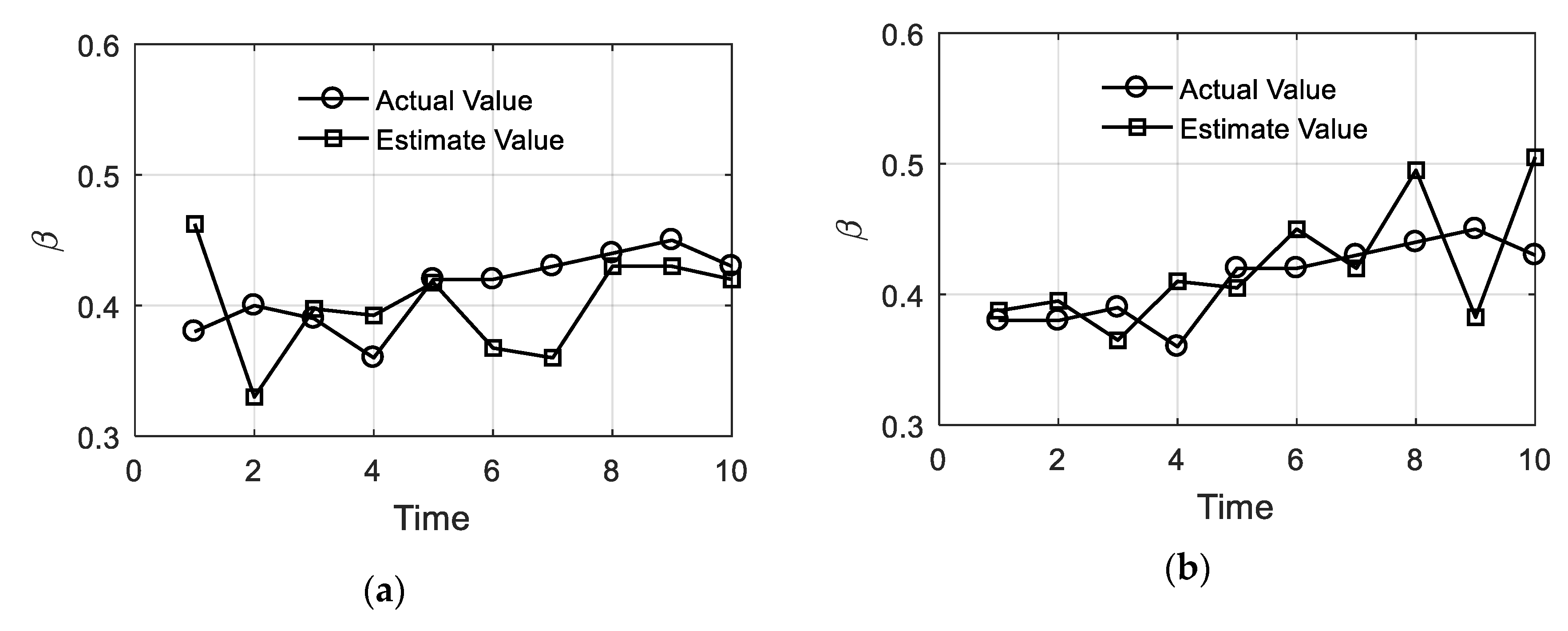
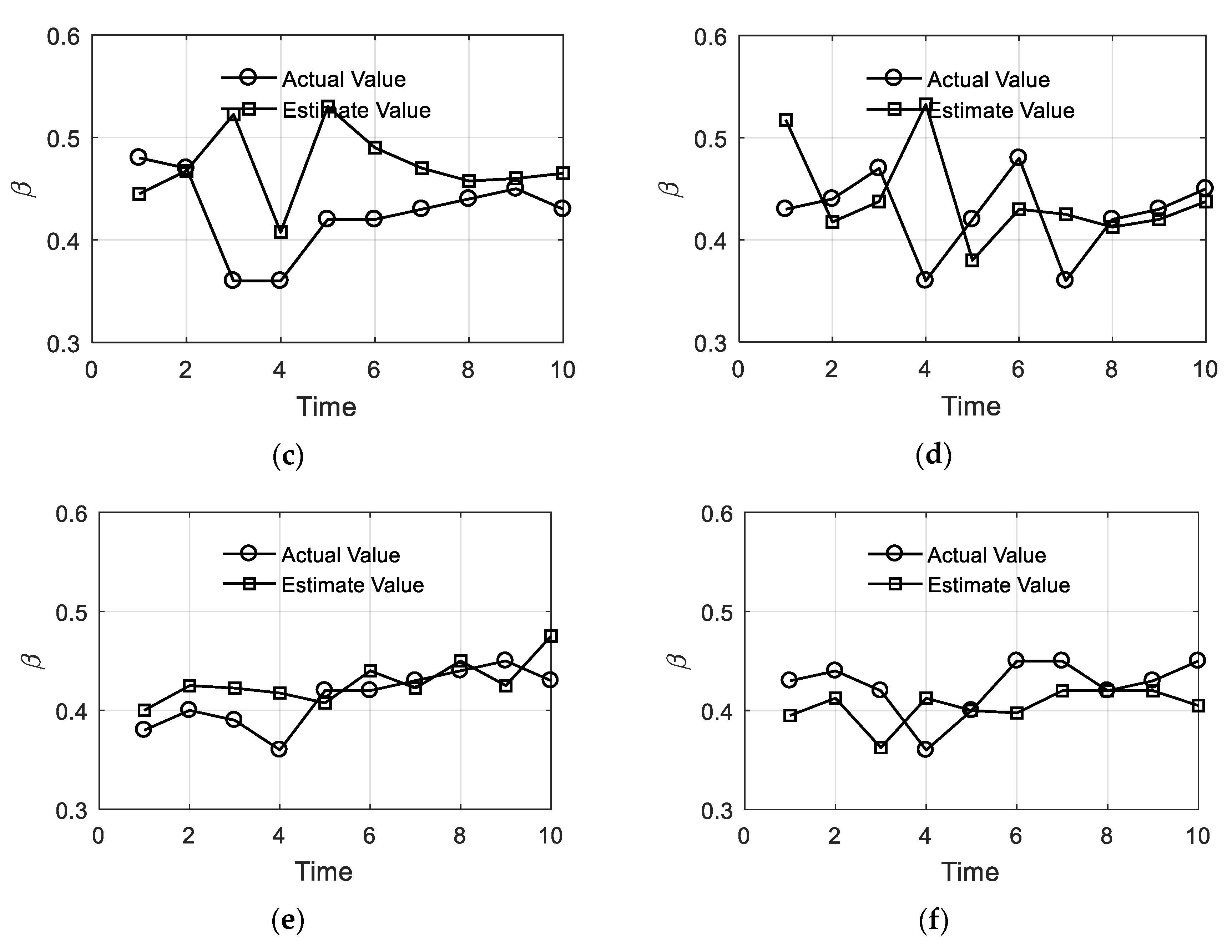
3.4. Impact of Information Feedback on Donations

A Mann–Whitney U test was used to compare the donations in Experiment 1 (C & NC) and Experiment 3 (C & NC), and Experiment 2 (C & NC) and Experiment 5 (C & NC), to study the impact of information feedback on the supply levels of goods for forestry infrastructure The specific results are shown in

Table 10. Mann–Whitney U test on the impact of information feedback on the supply levels of goods for forestry infrastructure.

Contrast Groups	P-Values	Contrast Groups	P-Values
Experiment 1 (NC) and Experiment 3 (NC)	0.009	Experiment 1 (C) and Experiment 3 (C)	0.496
Experiment 2 (NC) and Experiment 5 (NC)	0.028	Experiments 2(C) and Experiment 5 (C)	0.256

.

According to Table 10, when there was communication, information feedback had no significant impact on the supply levels of goods for forestry infrastructure. When there was no communication, the Mann–Whitney U-test results for Experiment 1 (NC) and Experiment 3 (NC) and Experiment 2 (NC) and Experiment 5 (NC) were significant. Combining this with Figure 2, it can be concluded that donations in Experiment 3 (NC) were higher than in Experiment 1 (NC) (C31 was higher than C11) and that donations in Experiment 2 (NC) were higher than in Experiment 5 (NC) (C21 was higher than C51), indicating that when the environment was determined, information feedback increased donations. When the environment was uncertain, a lack of information feedback increased donations.

3.5. Impact of Reward and Punishment on Donations

3.5.1. Statistical Analyses of Reward and Punishment

In order to indicate the impact of reward and punishment in different experimental scenarios, Figure 4 summarizes the four variables from Experiments 4 (C & NC) and 6 (C & NC): “average donation amounts for rewards”, “average donation amount for punishment”, “average reward received”, and “average penalty received”. In Figure 4, “A1, A2, A3, and A4” mean “average donation amounts for rewards”; “P1, P2, P3, and P4” mean “average donation amounts for punishment”; “A11, A21, A31, and A41” mean “average reward received”; and “P11, P21, P31, and P41” mean “average penalty received”.

In analyzing Figure 4, it can be seen that if there was no communication, the donations used for rewards declined, regardless of whether the environment was determined or not. Donations used for punishment fluctuated at around 1 in Experiment 4 (C & NC), while Experiment 6 (C & NC) showed an upward trend. In Experiment 4 (C & NC), rewards received had a downward trend, while in Experiment 6 (C & NC), they fluctuated steadily at around 1. In Experiment 4 (C & NC), penalties obtained fluctuated smoothly around 1, while in Experiment 6 (C & NC), they had an upward trend. In general, because there was no communication before making decisions, the intensity of reward and punishment after decision-making was relatively low, and the fluctuations in trends were relatively stable.

If there was communication, donations used for rewards increased in Experiment 4 (C & NC), while in Experiment 6 (C & NC), they decreased. Donations used for punishment were at 0 in Experiment 4 (C & NC), while in Experiment 6 (C & NC) they had an upward trend. In Experiment 4 (C & NC), rewards received had an upward trend, while in Experiment 6 (C & NC), they declined steadily. In Experiment 4 (C & NC), penalties obtained were at 0, while in Experiment 6 (C & NC), they had an upward trend. In general, with communication, the amount of money donated for reward and the amount of money donated for punishment were higher than the amounts given when there was no communication, and donations for reward or punishment fluctuated greatly.

3.5.2. Mann–Whitney U Test of Reward and Punishment Mechanisms

In order to analyze whether a reward and punishment mechanism significantly affected the supply level of goods for forestry infrastructure, a Mann–Whitney U test was used to compare the “mean value of donations without communication” to the “mean value of donations with communication” in Experiment 3 (C & NC) and Experiment 4 (C & NC) and in Experiment 5 (C & NC) and Experiment 6 (C & NC). The test results are shown in

Table 11. Mann–Whitney U test on the influence of reward and punishment on the supply level of goods for forestry infrastructure.

Contrast Groups	P-Values	Contrast Groups	P-Values
Experiment 3 (NC) and Experiment 4 (NC)	0.000	Experiment 3 (C) and Experiment 4 (C)	0.003
Experiment 5 (NC) and Experiment 6 (NC)	0.000	Experiment 5 (C) and Experiment 6 (C)	0.001

.

In analyzing Table 11, it can be concluded that a reward and punishment mechanism could significantly affect the supply level of goods for forestry infrastructure. In Figure 2, it can be seen that the average donation amount in Experiment 6 (NC) was significantly higher than that in Experiment 5 (NC) and that the average donation amount in Experiment 6 (C) was significantly higher than that in Experiment 5 (C), which indicates that setting up a reward and punishment mechanism could significantly increase the supply level of goods for forestry infrastructure. The reason is that, after a reward and punishment mechanism was set up, members would consider not only their own economic interests but also other social benefits such as reputation and fame while making decisions. Therefore, members would choose to increase their donations to obtain more benefits. Moreover, in the long term, the members of the community were fixed and could not avoid being punished due to the punishment mechanism. Therefore, members would choose to increase their donations in order to avoid punishment by other members.

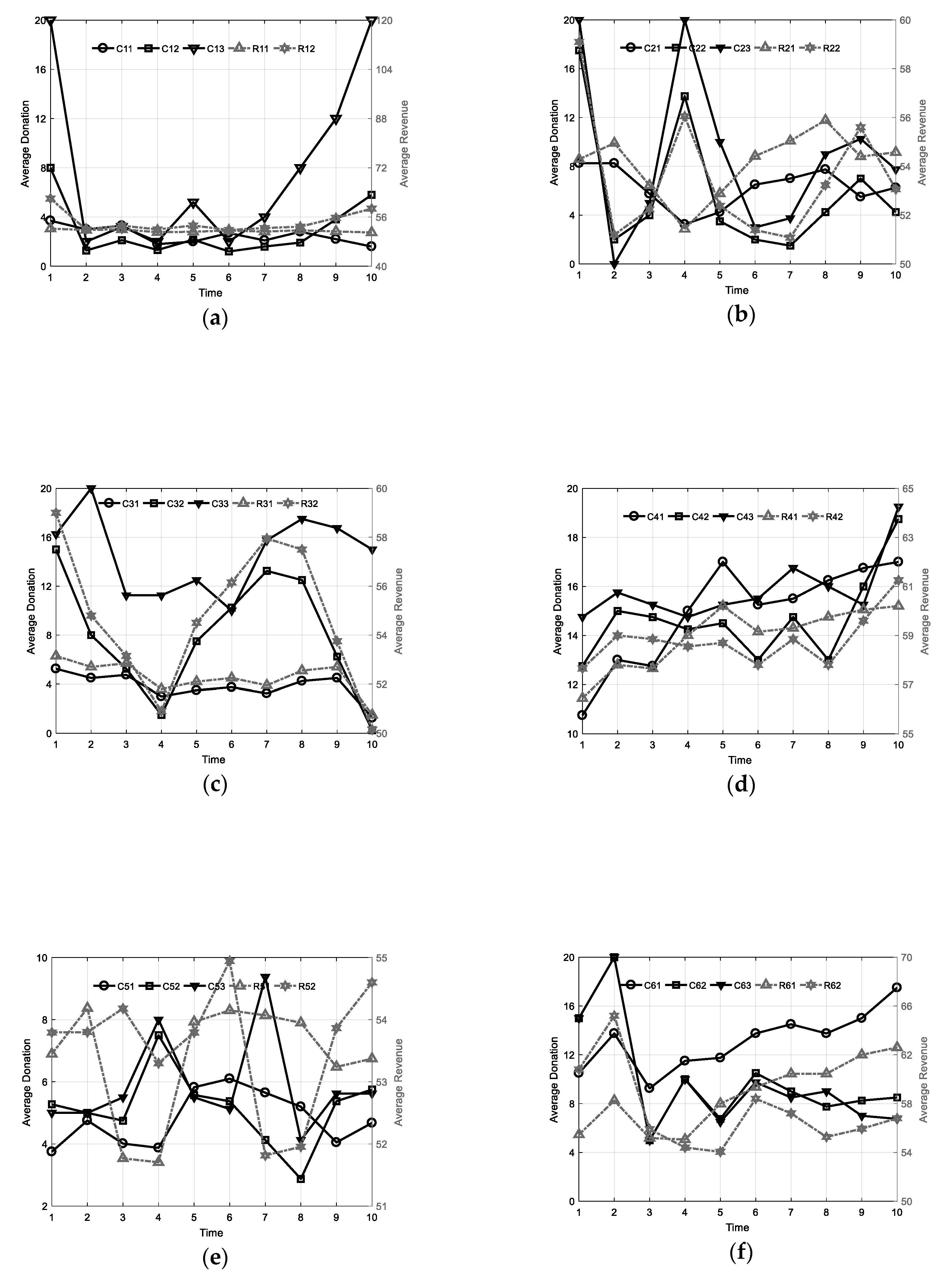
3.6. Research on the Influencing Factors on Donation Amounts in Different Experimental Situations

In order to study the influencing factors—the direction and degree of influence over the actual donation amounts due to different experimental mechanisms—a regression analysis on the data from the six groups of experiments were conducted.

3.6.1. Experiment 1 (C & NC)

Taking “actual donation amount without communication (ADNC)” and “actual donation amount with communication (ADC)” as dependent variables, and taking “planned donation (PD)”, “return from the previous round (R)”, and “degree of trust in strangers (S)” as independent variables, a regression was implemented. The results are shown in

Table 12. Regression analysis results for Experiment 1 (C & NC).

Independent Variables	Dependent Variables
	ADNC	ADC
PD	-	0.3806 ** (0.0779)
R	−2.0149 ** (0.2975)	0.0670 (0.1720)
S	−0.2046 (0.7246)	−0.1938 (0.9113)
Constant	110.5538 ** (15.8225)	−0.4205 (9.7951)
F	23.11 **	8.13 **
R2	0.5834	0.4326

Note: * significant at the 0.05 probability level; ** significant at the 0.01 probability level. ADNC: “actual donation amount without communication”; ADC: “actual donation amount with communication”.

.

Table 12 shows that at a 99% confidence level, the last round of earnings had a significant impact on the actual donation amount when there was no communication. For every unit increase in income in the previous round, the actual donation amount decreased by 2.0149 units when there was no communication. In this case, the increase in income in the previous round was due to reduced investment compared to other members and the extra income received through free-riding. Therefore, when income increased, less was invested. At a 99% confidence level, the planned donation amount had a significant impact on the actual donation amount when there was communication. For every unit increase in the planned donation amount, the actual donation amount increased by 0.3806 units when there was communication. The F-statistics were all significant.

3.6.2. Experiment 2 (C & NC)

The regression results for the dependent variables “actual donation amount without communication (ADNC)” and “actual donation amount with communication (ADC)”, as well as the independent variables “planned donation (PD)”, “estimated value of β (EV)”, “return from the previous round (R)”, the “actual value of β in the previous round (AV)”, and “degree of trust in strangers (S)” are shown in

Table 13. Regression analysis results for Experiment 2 (C & NC).

Independent Variables	Dependent Variables
	ADNC	ADC
PD	-	0.5395 ** (0.1226)
EV	21.7732 * (8.4576)	5.9781 (10.3440)
R	0.1414 (0.1747)	0.0170 (0.1591)
AV	−2.7987 (25.2626)	−2.5214 (25.4660)
S	0.5917 (1.5337)	−0.5469 (1.5920)
Constant	−11.3111 (13.5503)	−0.1530 (15.7398)
F	2.84 *	4.64 **
R2	0.2681	0.4363

Note: * significant at the 0.05 probability level; ** significant at the 0.01 probability level. ADNC: “actual donation amount without communication”; ADC: “actual donation amount with communication”.

.

Table 13 shows that at a 95% confidence level, the estimated value of β had a significant impact on the actual donation amount when there was no communication. For each unit increase in the estimated value of β, the actual donation amount increased by 21.7732 units when there was no communication. That is, the higher the estimated rate of return β was, the more confidence there was in investment prospects, and the more money was donated. At a 99% confidence level, the planned donation amount had a significant impact on the actual donation amount when there was communication. For every unit increase in the planned donation amount, the actual donation amount increased by 0.5395 units when there was communication. The F-statistics were all significant.

3.6.3. Experiment 3 (C & NC)

Taking “actual donation amount without communication (ADNC)” and “actual donation amount with communication (ADC)” as the dependent variables and “planned donation amount (PD)”, “return from last round (R)”, and “degree of trust in strangers (S)” as the independent variables, a regression was implemented, and the results are shown in

Table 14. Regression analysis results for Experiment 3 (C & NC).

Independent Variables	Dependent Variables
	ADNC	ADC
PD	-	0.3806 ** (0.0779)
R	0.8662 ** (0.0449)	0.0670 (0.1720)
S	−0.3889 ** (0.0743)	−0.1938 (0.9113)
Constant	−41.4704 ** (2.3666)	−0.4205 (9.7951)
F	199.73 **	8.13 **
R2	0.9237	0.4326

Note: * significant at the 0.05 probability level; ** significant at the 0.01 probability level. ADNC: “actual donation amount without communication”; ADC: “actual donation amount with communication”.

.

Table 14 shows that at a confidence level of 99%, the benefits received in the previous round and the degree of trust in strangers had a significant impact on the actual donation amount when there was no communication. For each additional unit of income received in the previous round, the actual donation amount increased by 0.8662 units when there was no communication. The increase in income could be attributed to an increase in the amount in the public account, which was caused by the overinvestment of group members. Therefore, there was a positive correlation between the benefits received in the previous period and the actual donation amount when there was no communication. For each additional unit in the “degree of trust in strangers (S)” variable, the actual donation amount when there was no communication decreased by 0.3889 units. At a 99% confidence level, the planned donation amount had a significant impact on the actual donation amount when there was communication: for every unit increase in the planned donation amount, the actual donation amount increased by 0.3806 units. The F-statistics were significant.

3.6.4. Experiment 4 (C & NC)

Taking the “actual donation amount without communication (ADNC)” and the “actual donation amount with communication (ADC)” as the dependent variables and the “planned donation amount (PD)”, “return from the previous round (R)”, “reward received from the previous round (RP)”, “penalty received from the previous round (PP)”, ”revenue after the previous round of reward and punishment (RRP)” and “degree of trust in strangers (S)” as the independent variables, a regression was implemented, the results of which are shown in

Table 15. Regression analysis results for Experiment 4 (C & NC).

Independent Variables	Dependent Variables
	ADNC	ADC
PD	-	0.9277 ** (0.1710)
R	−0.0372 (0.3619)	0.0014 (0.1615)
RP	−1.1947 (0.9250)	−0.3030 (0.5093)
PP	1.7193 (1.0083)	-
RRP	0.5720 * (0.2781)	0.0875 (0.0825)
S	0.8822 (0.5812)	0.0614 (0.3912)
Constant	−23.5713 (15.4177)	−6.2810 (12.5589)
F	1.93	6.60 **
R2	0.2434	0.5238

Note: * significant at the 0.05 probability level; ** significant at the 0.01 probability level. ADNC: “actual donation amount without communication”; ADC: “actual donation amount with communication”.

.

Table 15 shows that at a 95% confidence level, earnings after the previous round of reward and punishment had a significant impact on the actual donation amount when there was no communication. For each additional unit of earnings after the previous round of reward and punishment, the actual donation amount increased by 0.5720 units when there was no communication. At a 99% confidence level, the planned donation amount had a significant impact on the actual donation amount when there was communication. For every unit increase in the planned donation amount, the actual donation amount increased by 0.9277 units when there was communication.

3.6.5. Experiment 5 (C & NC)

Taking “the actual donation amount without communication (ADNC)” and “the actual donation amount with communication (ADC)” as the dependent variables and the “planned donation amount (PD)”, “estimated value of β (EV)”, “return from the previous round (R)”, “actual value of β in the previous round (AV)”, and “degree of trust in strangers (S)” as the independent variables, a regression was implemented. The results are shown in

Table 16. Regression analysis results for Experiment 5 (C & NC).

Independent Variables	Dependent Variables
	ADNC	ADC
PD	-	0.1941 (0.1338)
EV	1.7577 (3.1826)	9.4234 * (4.5536)
R	−0.6062 ** (0.1638)	−0.1654 (0.1859)
AV	5.7869 (7.3403)	2.8021 (9.3125)
S	−0.3296 (0.3630)	−0.4663 (0.4228)
Constant	34.7118 ** (7.7161)	8.6229 (8.8104)
F	5.34 **	3.49 *
R2	0.4081	0.3678

Note: * significant at the 0.05 probability level; ** significant at the 0.01 probability level. ADNC: “actual donation amount without communication”; ADC: “actual donation amount with communication”.

.

Table 16 shows that at a 99% confidence level, the earnings from the previous round had a significant impact on the actual amount of donations when there was no communication. For each unit increase in the previous round’s income, the actual amount of money donated decreased by 0.6062 units when there was no communication. If there was communication, the estimated value of β had a significant effect on the actual donation amount at a 95% confidence level. For each additional unit of the estimated value of β, the actual donation amount increased by 9.4234 units when there was communication. The F-statistics were significant.

3.6.6. Experiment 6 (C & NC)

Taking the “actual donation amount without communication (ADNC)” and the “actual donation amount with communication (ADC)” as the dependent variables and the “planned donation amount (PD)”, “return from the previous round (R)”, “reward received from the previous round (RP)”, “penalty received from the previous round (PP)”, “returns after one round of reward and punishment (RRP)”, “estimated value of β (EV)”, “actual value of β in the previous round (AV)”, and “degree of trust in strangers (S)” as the independent variables, a regression was implemented, the results of which are shown in

Table 17. Regression analysis results for Experiment 6 (C & NC).

Independent Variables	Dependent Variables
	ADNC	ADC
PD	-	0.8344 ** (0.0670)
R	−0.02810 (0.3152)	−0.0039 (0.1300)
RP	−0.03906 (1.2356)	0.2757 (0.6025)
PP	0.3405 (0.6826)	−0.4356 (0.3273)
RRP	0.1126 (0.1970)	−0.0865 (0.0952)
EV	15.9091 * (6.9543)	6.3467 (9.8157)
AV	65.7716 * (27.6774)	2.8950 (13.3299)
S	0.5950 (1.0832)	0.1638 (0.5813)
Constant	−12.5920 (11.7948)	3.9333 (7.2328)
F	2.43 *	28.50 **
R2	0.3780	0.8941

Note: * significant at the 0.05 probability level; ** significant at the 0.01 probability level. ADNC: “actual donation amount without communication”; ADC: “actual donation amount with communication”.

.

Table 17 shows that at a 95% confidence level, the estimated value of β had a significant effect on the actual donation amount when there was no communication. For each additional unit in the estimated β value, the actual donation amount increased by 15.9091 units when there was no communication. At a 95% confidence level, the actual value of β in the previous round had a significant impact on the actual donation amount when there was no communication. For each increase in the actual value of β in the previous round, the actual donation amount increased by 65.7716 units when there was no communication. At a 99% confidence level, the planned donation amount had a significant impact on the actual donation amount when there was communication. For every unit increase in the planned donation amount, the actual donation increased by 0.8344 units when there was communication. The F-statistics were significant.

4. Discussion and Conclusions

Two main issues were studied in this paper: (1) Which is better, cooperation or noncooperation? (2) What are the key factors affecting the private, voluntary supply of goods for forestry infrastructure? The following was found: (1) With private cooperation, the supply was higher than with private noncooperation. (2) Communication, environmental determination, information feedback, and reward and punishment mechanisms affected the quantity of private, voluntary supplies. (3) Communication could increase supply. (4) Reward and punishment mechanisms could also increase supply. (5) The impact of environmental certainty on supply depended on reward and punishment mechanisms. When there was no reward and punishment mechanism, environmental uncertainty increased the supply of goods for forestry infrastructure. When incentives and penalties were in place, a defined environment increased the supply of goods for forestry infrastructure. (6) The impact of information feedback on supply depended on environmental certainty. When the environment was determined, information feedback increased donations. When the environment was uncertain, no information feedback increased donations.

Choi and Ahn have written that rewards and punishments can increase supply [59]. This is consistent with our findings. Zhou and other scholars have indicated that environmental uncertainty could increase donations [58]. Zhou’s experimental design considered leaders and did not consider reward and punishment mechanisms, which is not exactly what our experimental design did. Zhang found that information feedback could affect free-riding behavior [61]. Our research did not consider the method of information feedback, which is a disadvantage of our experimental design.

The conclusions of our experiments are instructive for the private, voluntary provision of quasi-public goods for forestry infrastructure. On the one hand, low-cost quasi-public goods can be provided by private, voluntary foresters in a forest. Meanwhile, cooperation between forest farmers should be promoted as far as possible. On the other hand, reward and punishment mechanisms ought to be more public, and members should communicate more.

References

1. Hagadone, T.A.; Grala, R.D. Business clusters in Mississippi’s forest products industry. For. Policy Econ. 2012, 20, 16–24. [Google Scholar] [CrossRef]
2. Czajkowski, M.; Bartczak, A.; Giergiczny, M.; Navrud, S.; Zylicz, T. Providing preference-based support for forest ecosystem service management. For. Policy Econ. 2014, 39, 1–12. [Google Scholar] [CrossRef]
3. Atewamba, C.; Boimah, M. Policy forum: Potential options for greening the concessionary forestry business model in rural Africa. For. Policy Econ. 2017, 85, 46–51. [Google Scholar] [CrossRef]
4. Xu, H.W. On the application of forestry engineering cost management information. China For. Prod. Ind. 2015, 42, 56–57. [Google Scholar] [CrossRef]
5. Zhang, F.Y.; Du, J.; Kang, X.L.; Zhu, S.B. Empirical research on influencing factors and action mechanism of farmer’s forestry income. For. Econ. 2017, 39, 15–22. [Google Scholar]
6. Flatberg, T.; Nørstebø, V.S.; Bjørkelo, K.; Astrup, R.; Søvde, N.E. A mathematical model for infrastructure investments in the forest sector of coastal Norway. For. Policy Econ. 2018, 92, 202–209. [Google Scholar] [CrossRef]
7. Svetlana, P.; Jussi, H.; Esa, V. Policy forum: Challenges of forest governance: Biomass export from Leningrad Oblast, north-west of Russia. For. Policy Econ. 2018, 95, 13–17. [Google Scholar]
8. Falcone, P.M.; Tani, A.; Tartiu, V.E.; Imbriani, C. Towards a sustainable forest-based bioeconomy in Italy: Findings from a SWOT analysis. For. Policy Econ. 2020, 110, 101910. [Google Scholar] [CrossRef]
9. Akay, A.E.; Sessions, J. Roading and transport operations. In Encyclopedia of Forest Sciences; Burley, J., Evans, J., Youngquist, J., Eds.; Elsevier Academic Press: Amsterdam, The Netherlands, 2004; pp. 259–269. [Google Scholar]
10. Enache, A.; Pentek, T.; Ciobanu, V.D.; Stampfer, K. GIS based methods for computing the mean extraction distance and its correction factors in Romanian mountain forests. Šumar List. 2015, 139, 35–46. [Google Scholar]
11. Hayati, E.; Majnounian, B.; Abdi, E. Qualitative evaluation and optimization of forest road network to minimize total costs and environmental impacts. Forests 2012, 5, 121–125. [Google Scholar] [CrossRef] [Green Version]
12. Laschi, A.; Neri, F.; Brachetti Montorselli, N.; Marchi, E. A methodological approach exploiting modern techniques for forest road network planning. Croat. J. For. Eng. 2016, 37, 319–331. [Google Scholar]
13. Parsakhoo, A.; Mostafa, M. Road network analysis for timber transportation from a harvesting site to mills (Case study: Gorgan county–Iran). J. For. Sci. 2015, 61, 520–525. [Google Scholar] [CrossRef] [Green Version]
14. Picchio, R.; Latterini, F.; Mederski, P.S.; Venanzi, R.; Karaszewski, Z.; Bembenek, M.; Croce, M. Comparing accuracy of three methods based on the GIS environment for determining winching areas. Electronics 2019, 8, 53. [Google Scholar] [CrossRef] [Green Version]
15. Feng, Q.L.; Qin, F.D.; Liao, H.J.; Zhao, F.H. An empirical study on the influencing factors of the quality of poverty alleviation work of the forestry industry in Guangxi. For. Econ. 2018, 40, 26–32. [Google Scholar]
16. Su, S.P.; Wu, J.Y.; Gan, J.B. Comparative analysis of total factor productivity change among family forestry operators since forest tenure reform in Fujian, Zhejiang and Jiangxi provinces. Resour. Sci. 2015, 37, 112–124. [Google Scholar]
17. He, D.H.; Zhu, D.L. The collective forest tenure reform implementation and performance evaluation: 2014 monitoring observations of collective forest tenure reform. For. Econ. 2015, 37, 13–27. [Google Scholar]
18. Picchio, R.; Spina, R.; Calienno, L.; Venanzi, R.; Lo Monaco, A. Forest operations for implementing silvicultural treatments for multiple purposes. Ital. J. Agron. 2016, 11, 156–161. [Google Scholar]
19. Gumus, S.; Turk, Y. A new skid trail pattern design for farm tractors using linear programing and geographical information systems. Forests 2016, 7, 306. [Google Scholar] [CrossRef] [Green Version]
20. Zhu, H.Y.; Zhao, J.Y. Analysis on Chinese herbal medicine planting subsidies pilots. For. Econ. 2015, 37, 61–64. [Google Scholar]
21. Xue, Y.Z. Study on forest zone disaster-reduction indicator system construction and countermeasures in western China. Issues For. Econ. 2015, 35, 133–137. [Google Scholar]
22. Han, J.H.; Lin, H.J.; Zhang, J.Z. Analysis of people’s livelihood forestry developing in state forest zone: A study case in Chifeng forestry. For. Econ. 2015, 37, 75–79. [Google Scholar]
23. Chen, S.Z.; Bai, X.P. Support system for forestry-related disaster prevention and mitigation policy in Japan and its implications. World For. Res. 2014, 27, 67–74. [Google Scholar]
24. Song, W.Z.; Wang, A.J. Analysis of impacts and causes of ice and snow disasters: Taking bamboo forest in Zhejiang as an example. For. Resour. Manag. 2008, 37, 45–49. [Google Scholar]
25. Corona, P.; Ascoli, D.; Barbati, A.; Bovio, G.; Colangelo, G.; Elia, M.; Garfì, V.; Iovino, F.; Lafortezza, R.; Leone, V.; et al. Integrated forest management to prevent wildfires under Mediterranean environments. Ann. Silvic. Res. 2015, 39, 1–22. [Google Scholar]
26. Liao, B.; Gao, X.P.; Liao, W.M.; Zhang, G.L. A Comparative analysis on the structure of forestry fixed assets investment in Jiangxi. Issues For. Econ. 2014, 34, 154–159. [Google Scholar]
27. Sun, W.; Cao, S.S.; Pu, Z.; Fu, L.Y. Cloud infrastructure of forest resources information. J. Northwest For. Univ. 2014, 29, 71–79. [Google Scholar]
28. Pinkard, E.; Battaglia, M.; Bruce, J.; Matthews, S.; Callister, A.N.; Hetherington, S.; Last, I.; Mathieson, S.; Mitchell, C.; Mohammed, C.; et al. A history of forestry management responses to climatic variability and their current relevance for developing climate change adaptation strategies. Forestry 2015, 88, 155–171. [Google Scholar] [CrossRef] [Green Version]
29. Wang, Z.X.; Yan, H.W.; Mo, M. Some thoughts on forestry recovery and reconstruction after rain and snow freezing in the south of China. For. Resour. Manag. 2008, 37, 1–5. [Google Scholar]
30. Wu, B. Some Thoughts on forestry and ecological recovery and reconstruction in the southern rain and snow freezing areas. Sci. Silvae Sin. 2008, 54, 2–4. [Google Scholar]
31. Kong, F.B.; Liao, W.M. Forestry development effects of forestry marketization process in China: Based on statistical data of 31 Provinces (cities and autonomous regions) during 2002 to 2011. Sci. Silvae Sin. 2013, 49, 126–135. [Google Scholar]
32. Xiao, Z.; Chen, Y.G.; Zhou, Y. Dynamic relationship between public service investment and forestry economic growth: A study based on OLS regression initial model. Issues For. Econ. 2012, 32, 177–184. [Google Scholar]
33. Gordon, T. The economics of public choice/perspectives on public choice: A handbook. Econ. J. 1998, 108, 1886–1888. [Google Scholar]
34. Krauze, A. Let the public sector go free. New Statesman 2000, 129, 5. [Google Scholar]
35. Shen, M.H.; Xie, H.M. On the issue of public goods and its solution: A review on the public goods theory. J. Zhejiang Univ. (Hum. Soc. Sci.) 2009, 39, 133–144. [Google Scholar]
36. Li, S.S. An analysis of the disadvantages and countermeasures of the government’s provision of public goods. Party Sch. Le Shan Munic. Comm. C.P.C. 2011, 13, 45–47. [Google Scholar]
37. Henry, H. Ownership of the firm. J. Law Econ. Organ. 1988, 4, 267. [Google Scholar]
38. Savas, E.S. Privatization and Public-Private Partnerships; Renmin University of China Press: Beijing, China, 2002; pp. 57–321. [Google Scholar]
39. Fu, J.L.; Cui, H.; Huang, X.H. Farmers’ voluntary provision of public goods in rural communities: Analysis based on the theory of reputation. Econ. Surv. 2007, 24, 106–109. [Google Scholar]
40. Hong, B.G.; Zhang, Y.B. Rent-seeking game analysis on quasi-public goods supplied by private in rural areas: Rural passenger transport system as an example. J. Xiangtan Univ. (Philos. Soc. Sci.) 2009, 33, 44–48. [Google Scholar]
41. Xiao, W.; Zhu, Y.Z. Game analysis of the supply of rural public goods on the basis of contracts: Taking the rural areas of Hunan province as an example. Chin. Rural. Econ. 2010, 29, 26–36. [Google Scholar]
42. Liu, B.X.; Liu, W.L. Game analysis of private supply mechanism of quasi-public goods: Taking Chinese transportation infrastructure investment as an example. China Soft Sci. 2007, 22, 145–151. [Google Scholar]
43. Liu, C.L.; Xu, Y.Q. The application of game model of public goods in information resources sharing in China. Inf. Sci. 2007, 28, 50–53. [Google Scholar]
44. Dong, Z.Y. Experimental Economics; Peking University Press: Beijing, China, 2008; pp. 8–11. [Google Scholar]
45. Rami, S.; David, V.B.; Amnon, R. Provision of step-level public goods with uncertain provision threshold and continuous contribution. Group Decis. Negot. 2001, 10, 253–274. [Google Scholar]
46. Jane, S.; Rick, K.W. Levels of information and contributions to public goods. Soc. Forces 1991, 70, 107–124. [Google Scholar]
47. Weimann, J. Individual behavior in a free riding experiment. J. Public Econ. 1994, 54, 185–200. [Google Scholar] [CrossRef]
48. Croson, R.T.A. Feedback in voluntary contribution mechanisms: An experiment in team production. Res. Exp. Econ. 2001, 8, 85–97. [Google Scholar]
49. Bigoni, M.; Suetens, S. Feedback and dynamics in public good experiments. J. Econ. Behav. Organ. 2012, 82, 86–95. [Google Scholar] [CrossRef]
50. Irlenbusch, B.; Ter Meer, J. Fooling the nice guys: Explaining receiver credulity in a public good game with lying and punishment. J. Econ. Behav. Organ. 2013, 93, 321–327. [Google Scholar] [CrossRef]
51. Huang, G.B.; Zhou, Y.A. Review of leadership research in experiment economics. Econ. Theory Bus. Manag. 2014, 34, 48–59. [Google Scholar]
52. Zhou, Y.; Zhang, Q.L.; Fu, L.; Yang, Y.Z.; Sun, G.Y. Effect of information disclosure mechanism on free riding behavior: Evidence from laboratory. J. Manag. Sci. China 2014, 17, 86–94. [Google Scholar]
53. Nikos, N. Feedback, Punishment and cooperation in public good experiments. Games Econ. Behav. 2010, 68, 689–702. [Google Scholar]
54. Faillo, M.; Grieco, D.; Zarri, L. Legitimate punishment, feedback and the enforcement of cooperation. Games Econ. Behav. 2013, 77, 271–283. [Google Scholar] [CrossRef] [Green Version]
55. Xie, S.Y. Economic Game Theory; Fudan University Press: Shanghai, China, 2017; pp. 23–24. [Google Scholar]
56. Klaus, R. Foundations of Non-Cooperative Game Theory; Oxford University Press: Oxford, UK, 2003; pp. 7–8. [Google Scholar]
57. Guo, X.J. Research on the Problem about the Private Provision of Quasi-Public Goods in China from the Perspective of Game Theory. Master’s Thesis, Shanxi University of Finance & Economics, Shanxi, China, 2016. [Google Scholar]
58. Zhou, Y.A.; Huang, G.B.; He, H.R.; Liu, M.W. Can leaders really serve as role models: A study based on public goods game experiments. Manag. World 2014, 30, 75–90. [Google Scholar]
59. Choi, J.-K.; Ahn, T.K. Strategic reward and altruistic punishment support cooperation in a public goods game experiment. J. Econ. Psychol. 2013, 35, 17–30. [Google Scholar] [CrossRef]
60. Hai, J.J. Research on Cooperative Behavior in Public Goods Game Experiment under Leadership-chasing Random System. Ph.D. Thesis, Shan Dong University, Shandong, China, 2018. [Google Scholar]
61. Zhang, J.B. Free Rider Behavior of Public Goods Based on Experimental Economics. Master’s Thesis, Beijing University of Posts and Telecommunications, Beijing, China, 2014. [Google Scholar]
Figure 1. Economic analysis of the private joint provision of forestry infrastructure.
Sustainability 12 02808 g001
Figure 2. The average donation amount for each period in the experiments with and without communication: (a) the statistics for average donations and average returns in Experiment 1 (C & NC); (b) statistics for average donations and average returns in Experiment 2 (C & NC); (c) statistics for average donations and average returns in Experiment 3 (C & NC); (d) statistics for average donations and average returns in Experiment 4 (C & NC); (e) statistics for average donations and average returns in Experiment 5 (C & NC); (f) statistics for average donations and average returns in Experiment 6 (C & NC). “Mean values of donations without communication”, “mean values of donations with communication”, “mean values of planned investment after communication”, “mean values of earnings without communication”, and “mean values of earnings with communication” represent the number of experimental coins under different experimental conditions. Before each round of experiments began, each member had 50 initial coins. “Time” is the number of rounds in the experiment, and 1–10 represents rounds 1–10. Each experiment had 10 rounds.
Sustainability 12 02808 g002
Figure 3. The average estimated and actual value of the rate of return β in each period: (a) under the conditions of Experiment 2 (NC), when the group members could not communicate (statistics on the estimated and true value of the rate of return β); (b) under the conditions of Experiment 2 (C), when the group members could communicate (statistics on the estimated and true value of the rate of return β); (c) under the conditions of Experiment 5 (NC), when the group members could not communicate (statistics on the estimated and true value of the rate of return β); (d) under the conditions of Experiment 5 (C), when the group members could communicate (statistics on the estimated and true value of the rate of return β); (e) under the conditions of Experiment 6 (NC), when the group members could not communicate (statistics on the estimated and true value of the rate of return β); (f) under the conditions of Experiment 6 (C), when the group members could communicate (statistics on the estimated and true value of the rate of return β). “Actual value” and “estimated value” represent the number of experimental coins under different experimental conditions. Before each round of experiments began, each member had 50 initial coins. “Time” is the number of rounds in the experiment, and 1–10 represents rounds 1–10. Each experiment contains 10 rounds.
Sustainability 12 02808 g003aSustainability 12 02808 g003b
Figure 4. Summary of reward and punishment in the groups with reward and punishment: (a) under the conditions of Experiment 4 (C & NC), when the group members could not communicate (statistics on rewards and punishments meted out to other people or statistics on rewards and punishments received by members); (b) under the conditions of Experiment 4 (C & NC), when the group members could communicate (statistics on rewards and punishments meted out to other people or statistics on rewards and punishments received by members); (c) under the conditions of Experiment 6 (C & NC), when the group members could not communicate (statistics on rewards and punishments meted out to other people or statistics on rewards and punishments received by members); and (d) under the conditions of Experiment 6 (C & NC), when the group members could communicate (statistics on rewards and punishments meted out to other people or statistics on rewards and punishments received by members). “Average donation amount for rewards”, “average donation amount for punishment”, “average reward received”, and “average penalty received” represent the number of experimental coins under different experimental conditions. Before each round of experiments began, each member had 50 initial coins. “Time” is the number of rounds in the experiment, and 1–10 represents rounds 1–10. Each experiment had 10 rounds.
Sustainability 12 02808 g004aSustainability 12 02808 g004b