Exploring Potential Pathways toward Energy-Related Carbon Emission Reduction in Heavy Industrial Regions of China: An Input–Output Approach

Abstract

It is a very urgent issue to reduce energy-related carbon emissions in China. The three northeastern provinces (Heilongjiang (HLJ), Jilin (JL), and Liaoning (LN)) are typical heavy industrial regions in China, playing an important role in the national carbon emission reduction target. In this study, we analyzed the energy consumption, carbon dioxide (CO₂) emissions, and CO₂ emission intensity of each sector in the three regions, and we compared them with the national level and those of China’s most developed province Guangdong (GD). Then, based on an input–output (I–O) framework, linkage analysis of production and CO₂ emission from sector–system and sector–sector dimensions was conducted. The results showed that the three regions accounted for about 1/10 of China’s energy consumption and 1/6 of China’s CO₂ emissions in 2012. In addition, the level of energy structure, CO₂ emission intensity, and sectoral structure lagged behind China’s average level, much lower than those for GD. According to the sectoral characteristics of each region and unified backward/forward linkages of production and CO₂ emissions, we divided sectoral clusters into those whose development was to be encouraged and those whose development was to be restricted. The results of this paper could provide policy–makers with reference to exploring potential pathways toward energy-related carbon emission reduction in heavy industrial regions.

1. Introduction

Greenhouse gas (GHG) emissions led to a series of environmental problems including the greenhouse effect [1]. As the main component of GHG, energy-related carbon emissions account for more than 80% of the world’s anthropogenic emissions [2]. From 1751 to 2012, China accounted for 10.7% of the world’s cumulative energy-related carbon dioxide (CO₂) emissions. China’s carbon emission accounted for a high proportion in the world, which was 26.9% in 2012 [3]. The State Council of China formulated three phases of policies on energy conservation and emission mitigation in the “five-year” cycle and made some achievements [4,5,6]. However, as the largest developing country, China is still facing great challenges in controlling energy consumption and CO₂ emissions on the premise of ensuring stable economic development [7,8].

It was proposed in China’s 13th Five-Year Plan (2016–2020) that the energy intensity and carbon intensity should decrease by 15% and 18%, respectively. Considering the heterogeneity of regional social and economic conditions, the targets should be further subdivided [9,10]. As a typical heavy industrial region, northeastern China (Heilongjiang (HLJ), Jilin (JL), and Liaoning (LN), see Figure 1) warrants more attention [11]. Establishment of an industrial foundation in the northeast of China was proposed in China’s first two Five-Year Plans (1953–1957, 1958–1962). Subsequently, an energy-based and emission-intensive economic development model was formed in the above three regions. At that stage, the economy in northeastern China grew rapidly until the early 1980s when the government shifted the focus to coastal regions by implementing economic reforms. However, due to the unsuitable industrial structure and relatively higher energy intensity, the energy-related CO₂ emissions in these three heavy industrial regions increased rapidly in recent years [12,13]. In 2012, the energy production and consumption (standard coal) in these three regions accounted for 13.72% and 9.45% of China’s total, respectively [14]. Even though there is a conflict between economic development and mitigation of CO₂ emissions, it is critical to find a potential pathway toward energy-related carbon emission reduction in the three heavy industrial regions [15].

The input–output (I–O) model was explored to investigate the interdependence among various sectors in an economy [16] and then applied in the environmental fields to quantify pollutant emissions in the consumption of intermediate inputs and final products [17,18,19]. Because of the characteristics of being easily applied to all sectors regardless of the length and complexity of the production chains, the I–O model was widely applied to the analysis of sector–sector linkage on CO₂ and pollutant emissions [20,21,22]. In addition, the I–O model makes it possible to measure both direct CO₂ emissions in production processes and indirect CO₂ emissions embodied in intermediate inputs [23]. Many scholars applied I–O models to analyze energy-related carbon emissions from different perspectives. However, most of them carried out empirical studies at the national level [24,25,26,27]. For a vast country, the industrial structure and economic level of provinces/states are different, which should bring difficulties in seeking an accurate spatial calculation of CO₂ emissions for a country [28]. As far as we know, the studies focusing on regional carbon emissions of large countries were limited to some developed regions or cities such as Beijing [29,30], six large Japanese cities [31], and Guangdong Province [32]. There are few studies focusing on regions where heavy industries dominate the economy. Therefore, this study aims to analyze the characteristics of CO₂ emissions in typical heavy industrial regions in China based on the I–O model and to seek a sustainable development path.

This study intends to make a holistic assessment of sector–sector and sector–system linkages of production and energy-related CO₂ emissions in heavy industrial regions (HLJ, JL, and LN) in 2012 and make a comparison with those of the whole nation and a developed province Guangdong (GD). In detail, regional sectoral energy type and consumption are analyzed. The sectoral CO₂ emissions and CO₂ emission intensity are calculated based on the terminal fossil fuel consumption model proposed by the Intergovernmental Panel on Climate Change (IPCC). Then, the production and energy-related CO₂ emissions linkages are measured within an I–O framework. The sector–sector linkage analysis helps to explore the effects (production and CO₂ emissions) of the changes in final demand or intermediate inputs of one sector on other sectors. The sector–system linkage analysis is used to investigate how the entire economy or the total CO₂ emissions are affected by the changes in final demand or intermediate inputs of one sector. According to the sectoral characteristics of each region and unified backward/forward linkages of production and CO₂ emissions, encouraged and constrained sectoral clusters are finally proposed.

2. Methods and Data

2.1. Energy-Related CO₂ Emissions

The CO₂ emissions are calculated by the terminal energy consumption model proposed by the Intergovernmental Panel on Climate Change (IPCC) [33]. Regional total and sectoral CO₂ emissions are calculated using the following equation:

$$C={{\displaystyle \sum }}_{i=1}^n{{\displaystyle \sum }}_{j=1}^m{C}_{ij}={{\displaystyle \sum }}_{i=1}^n{{\displaystyle \sum }}_{j=1}^m{E}_{ij}{F}_j,$$

(1)

where C, E, and F are the total CO₂ emissions, the terminal fossil fuel (coal equivalent) consumption, and the CO₂ emission coefficients, respectively. Superscript n and m refer to the number of fossil fuel types and the number of sectors, respectively. Subscript i and j denote the i-th fossil fuel and the j-th sector, respectively. The original fossil fuel consumption data are converted into coal equivalent according to the conversion coefficients. Sectoral CO₂ emission intensity (CI_j) is determined by the sectoral output and CO₂ emissions as follows:

$$C{I}_j=\frac{C_j}{X_j},$$

(2)

where $X_j$ is the output of the j-th sector.

2.2. Non-Competitive Environmentally Extended I–O Framework

The rows in the basic form of the I–O table describe the distribution of producer’s output throughout the whole system, while the columns describe the input composition required by a particular sector [34]. In the applied I–O analysis, the distinction between domestically produced and imported inputs cannot be negligible. In order to avoid overestimation of the multiplier effect of a given sector, the linkage calculation should only consider domestically supplied inputs [27]. As an open economic entity, China and regions import and export a great amount of goods/services [35]. Therefore, this study uses a non-competitive I–O table to reorganize the imports used as intermediate inputs ($m_{ij}$) and final demand ($m_i^f$). The critical assumption used for eliminating imports is that each final demand category and each sector use the imports with the same proportions [36,37]. The structure of extended I–O table with non-competitive import assumption is shown in

Table 1. Structure of non-competitive environmentally extended input–output table.

		Intermediate Use	Final Demand	Total Output
Intermediate inputs	Domestic inputs	$x_{ij}^d$	$Y_i^d$	$X_i$
	Imports	$m_{ij}$	$m_i^f$	$m_i$
Primary input		$Z_j$
Total input		$X_j$
CO2 emission		$C_j$

. Domestic supplies and imports are decomposed into two rows as shown in Table 1. Intermediate inputs consist of domestically produced products used as inputs ($x_{ij}^d$) and imported products used as inputs ($m_{ij}$).

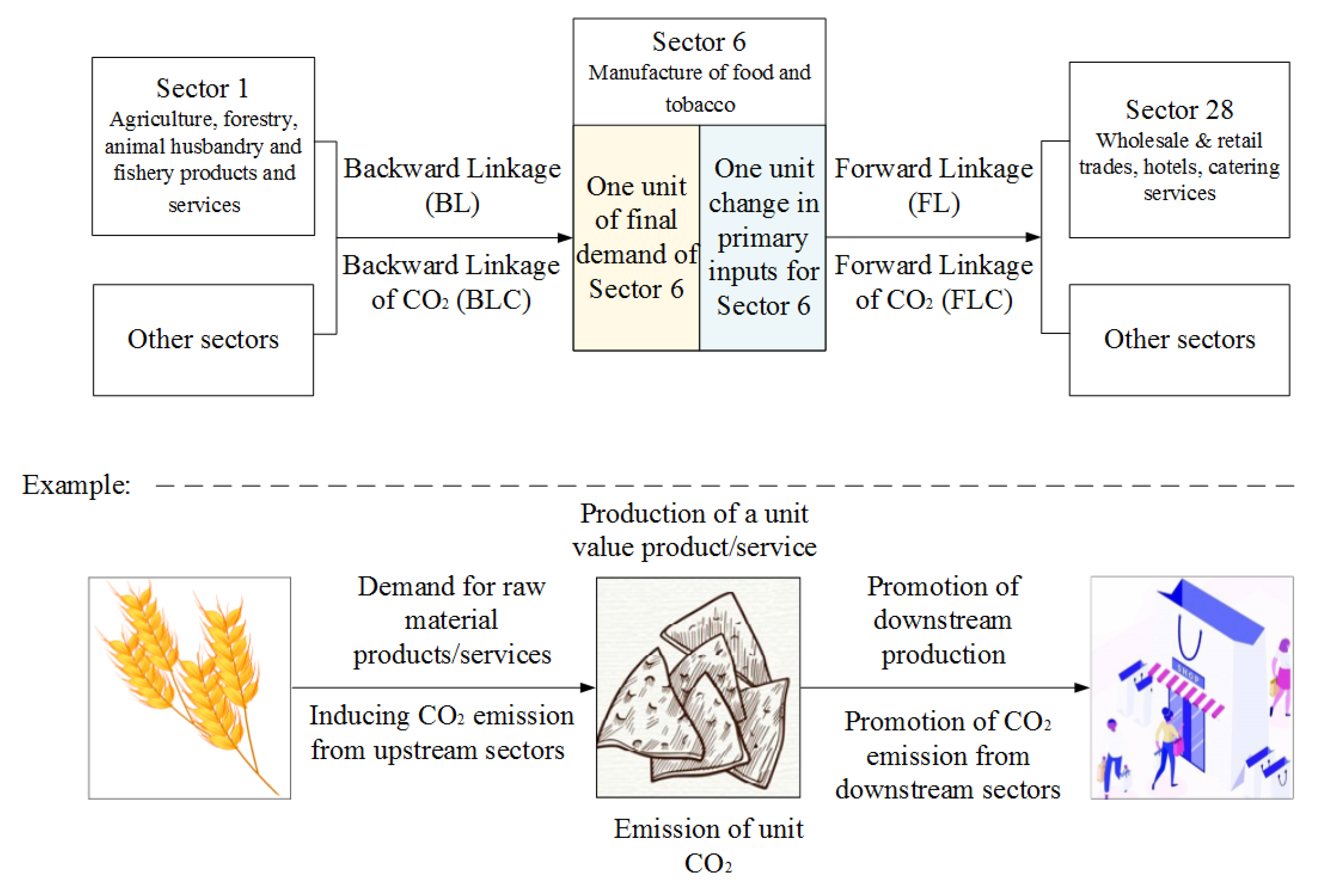
2.3. Production and CO₂ Emission Linkages Model

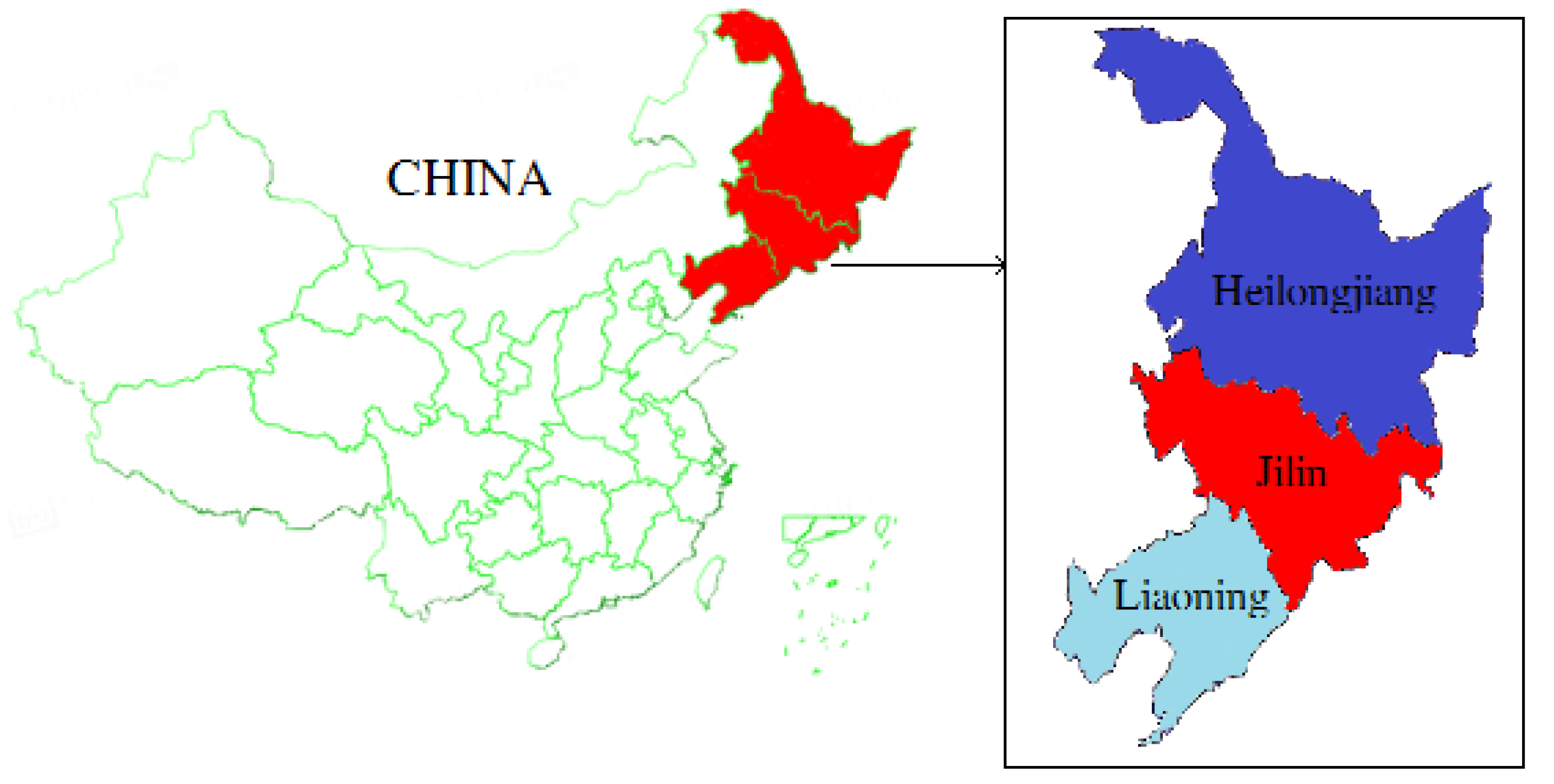
Based on the non-competitive environmentally extended I–O framework, we define that the direction of $x_{ij}$ is from sector i to sector j. In order to describe the relationship between two sectors, there are two concepts proposed by Leontief [16] and Ghosh [38], as shown in Equations (3) and (4), respectively.

$$\mathrm{A}=\left\{A_{ij}\right\}=\left\{\frac{x_{ij}}{X_j}\right\}=\left\{\frac{x_{ij}^d}{X_j}\right\}+\left\{\frac{m_{ij}}{X_j}\right\},$$

(3)

$$\mathrm{B}=\left\{B_{ij}\right\}=\left\{\frac{x_{ij}}{X_i}\right\}=\left\{\frac{x_{ij}^d}{X_i}\right\}+\left\{\frac{m_{ij}}{X_i}\right\},$$

(4)

where $A_{ij}$ denotes the input coefficients, and $B_{ij}$ represents the output coefficients. Equations (3) and (4) can be respectively expressed as follows:

$$\mathrm{A}=A^d+A^m,$$

(5)

$$\mathrm{B}=B^d+B^m,$$

(6)

where $A^d$ denotes the domestic input coefficient matrix (domestically produced goods/services), $B^d$ is the domestic output coefficient matrix, and $A^m$ and $B^m$ are imported input and output coefficient matrices, respectively.

$A^d$ and $B^d$ are used to express the direct linkage between two sectors. However, indirect linkages are generated among sectors in production chains. Therefore, it is necessary to calculate the total linkage among sectors. The matrices of once-indirect Leontief (Ghosh) coefficients among sectors are as follows:

$$A^d{}^2=\left(\begin{array}{cc}{a}_{ii}^d{}^2+a_{ij}^d{a}_{ji}^d& a_{ij}^d{a}_{ii}^d+a_{jj}^d{a}_{ij}^d\\ a_{ij}^d{a}_{ji}^d+a_{ji}^d{a}_{jj}^d& a_{jj}^d{}^2+a_{ji}^d{a}_{ij}^d\end{array}\right),$$

(7)

$$B^d{}^2=\left(\begin{array}{cc}{b}_{ii}^d{}^2+b_{ij}^d{b}_{ji}^d& b_{ij}^d{b}_{ii}^d+b_{jj}^d{b}_{ij}^d\\ b_{ij}^d{b}_{ji}^d+b_{ji}^d{b}_{jj}^d& b_{jj}^d{}^2+b_{ji}^d{b}_{ij}^d\end{array}\right).$$

(8)

The Leontief/Ghosh coefficients matrices (A_T/B_T) have the following equilibrium formulas:

$$A_T+I=I+A^d+A^d{}^2+A^d{}^3+\cdots +A^d{}^{\left(k+1\right)}+\cdots ={\left(I-A^d\right)}^{-1}=\left\{B{L}_{ij}\right\},$$

(9)

$$B_T+I=I+B^d+B^d{}^2+B^d{}^3+\cdots +B^d{}^{\left(k+1\right)}+\cdots ={\left(I-B^d\right)}^{-1}=\left\{F{L}_{ij}\right\},$$

(10)

where (k + 1) represents the k-th indirect Leontief (Ghosh) coefficients among sectors ($k\to \infty$, $A^d{}^{\left(k+1\right)}\to 0$). ${\left(I-A^d\right)}^{-1}$ and ${\left(I-B^d\right)}^{-1}$ represent the matrices of backward linkage (BL) and forward linkage (FL) between two sectors, also known as the Leontief inverse matrix and Ghosh inverse matrix, respectively.

(I) Sector–sector linkages of production and CO₂ emissions:

The sum of each column of the Leontief (row of Ghosh) inverse matrix is calculated to obtain the $B{L}_j$ ($F{L}_i$), which indicates the output of all sectors generated from the unit final demand of sector j (the effect on output of all sectors of unit change in primary inputs for sector i). BL and FL between two sectors are not simple reciprocal relations. Figure A1 (Appendix A) illustrates these two indicators with a simple example.

$$B{L}_j={{\displaystyle \sum }}_{i=1}^n{\alpha }_{ij}^d,$$

(11)

$$F{L}_i={{\displaystyle \sum }}_{j=1}^n{\beta }_{ij}^d,$$

(12)

where ${{\displaystyle \sum }}_{i=1}^n{\alpha }_{ij}^d$ and ${{\displaystyle \sum }}_{j=1}^n{\beta }_{ij}^d$ are the i-th row and j-th column elements of the matrix ${\left(I-A^d\right)}^{-1}$ and ${\left(I-B^d\right)}^{-1}$, respectively.

Equations (11) and (12) show the sector–sector backward and forward linkages from an economic point of view, respectively. Then, CO₂ emission intensity (CI) is introduced into Equations (11) and (12) to formulate sector–sector backward ($BL{C}_j$) and forward ($FL{C}_i$) linkages of CO₂ emissions.

$$BL{C}_j={{\displaystyle \sum }}_{i=1}^{n}C{I}_i{\alpha }_{ij}^d,$$

(13)

$$FL{C}_i={{\displaystyle \sum }}_{j=1}^n{\beta }_{ij}^{d}C{I}_j.$$

(14)

(II) Sector–system linkages of production and CO₂ emissions:

In order to better compare the degree of the linkages between sector and system (the entire economy), $B{L}_j$ and $F{L}_i$ are standardized to obtain the unified backward linkage (UBL) and unified forward linkage (UFL) in terms of production.

$$UB{L}_j=\frac{B{L}_j}{\frac{1}{m}{{\displaystyle \sum }}_{j=1}^{m}B{L}_j},$$

(15)

$$UF{L}_i=\frac{F{L}_i}{\frac{1}{m}{{\displaystyle \sum }}_{i=1}^{m}F{L}_i} .$$

(16)

$UB{L}_j$ and $UF{L}_i$ are capable of reflecting the effect of unitary change in final demand for sector j and primary inputs to sector i on the entire economy, respectively. If $UB{L}_j$ > 1, a unitary increase in final demand for sector j generates an above-average increase in the entire economy. If $UF{L}_i$ > 1, a unitary increase in primary inputs to sector i leads to an above-average increase in the entire economy. Accordingly, if $UB{L}_j$ > 1 and $UF{L}_i$ > 1, this sector can be recognized as a key sector in terms of economy. Therefore, it influences the whole economy to a great extent. In contrast, if $UB{L}_j$ < 1 and $UF{L}_i$ < 1, this sector can be recognized as a non-significant sector. Equations (15) and (16) show sector–system production linkages from an economic point of view. Sector–system linkages of CO₂ emissions are formed as follows:

$$UBL{C}_j=\frac{BL{C}_j}{\frac{1}{m}{{\displaystyle \sum }}_{j=1}^{m}BL{C}_j},$$

(17)

$$UFL{C}_i=\frac{FL{C}_i}{\frac{1}{m}{{\displaystyle \sum }}_{i=1}^{m}FL{C}_i}.$$

(18)

A similar interpretation can be adopted to CO₂ emission linkages. $UBL{C}_j$ > 1 indicates that a unitary increase in the final demand for sector j draws an above-average increase in CO₂ emissions, and $UFL{C}_i$ > 1 represents that a unitary increase in the primary inputs to sector i leads to an above-average increase in CO₂ emissions. The relatively small changes in the sectors ($UBL{C}_j$ > 1 and $UFL{C}_i$ > 1) which are defined as the key sectors in terms of CO₂ emissions could greatly affect the total CO₂ emissions in an economy. Therefore, industrial restructuring provides a potential pathway to reduce CO₂ emissions with relatively less negative effects on the economy through establishing two sectoral groups: constrained group ($UB{L}_j$ < 1, $UF{L}_i$ < 1, $UBL{C}_j$ > 1, and $UFL{C}_i$ > 1) and encouraged group ($UB{L}_j$ > 1, $UF{L}_i$ > 1, $UBL{C}_j$ < 1, and $UFL{C}_i$ < 1).

2.4. Data

This study focuses on sector–sector and sector–system linkages of production and energy-related CO₂ emissions in three heavy industrial regions (HLJ, JL, and LN). Simultaneously, linkage measurements for China and GD (a developed region) are also conducted for a comparative analysis. Two databases need to be established: an economic database and an energy-related CO₂ emission database. The economic database includes sectoral output and I–O relationships of China and four regions. Sectoral output data are used to calculate CO₂ emission intensity (see Equation (2)). The original I–O tables are used to produce extended I–O tables with non-competitive import assumption (see Table 1). These data are directly obtained from the I-O tables published by the Chinese Input–Output Association in 2016 and the three provinces’ Statistical Yearbooks in 2015 (the latest published I–O tables) [39,40,41,42]. The establishment of the sectoral energy-related CO₂ emission database requires the sectoral terminal energy consumption (physical unit) and CO₂ emission coefficient of each fossil fuel (proposed by the IPCC) as the original data (see Equation (1)). These original data are obtained from the China Energy Statistical Yearbook and the Statistical Yearbooks of three provinces in 2012 [14,43,44,45]. Sectoral energy-related CO₂ emissions are used to quantify sectoral CO₂ emission intensity. The extended I–O tables and sectoral CO₂ emission intensity are applied to calculate input and output coefficients (see Equations (3) and (4)), the basic equilibrium relationships (see Equations (5) and (6)), Leontief/Ghosh coefficient matrixes (see Equations (7)–(10)), sector–sector linkages (see Equations (11)–(14)), and sector–system linkages (see Equations (15)–(18)).

The classifications of sectors among these original data are different. According to the research purpose and data availability, the sectors are aggregated into 29 sectors (see

Table 2. Classification of aggregate sectors.

Sector Code	Sectors
S1	Agriculture, forestry, animal husbandry, and fishery products and services
S2	Mining and washing of coal
S3	Extraction of petroleum and natural gas
S4	Mining and processing of metal ores
S5	Mining and processing of non-metal ores
S6	Manufacture of food and tobacco
S7	Manufacture of textile
S8	Manufacture of textile, wearing apparel, shoes, hats, leather, feather, and related products
S9	Processing of wood, bamboo, rattan, palm, and straw products and manufacture of furniture
S10	Manufacture of paper and paper products; education and sport activities
S11	Petroleum processing and coking
S12	Manufacture of chemical products
S13	Manufacture of non-metallic mineral products
S14	Smelting and calendaring of metals
S15	Manufacture of metal products
S16	Manufacture of general and special purpose machinery
S17	Manufacture of transport equipment
S18	Manufacture of electrical machinery and equipment
S19	Manufacture of communication equipment, computer and other electronic equipment
S20	Other manufacturing industries
S21	Waste material
S22	Repair services for metal products, machinery, and equipment
S23	Production and supply of heat and electricity
S24	Production and supply of gas
S25	Production and supply of water
S26	Construction
S27	Transport, storage, and post
S28	Wholesale, retail trades, hotels, and catering services
S29	Other service sectors a

^a “Information and communication”, “financial and insurance activities”, “real estate activities”, “professional, scientific and technical activities”, “administrative and support service activities”, “public administration and defense; compulsory social security”, “education”, “human health and social work activities” and “arts, entertainment and recreation”.

). It must be pointed out that, when discussing environmental issues, the splitting and restructuring of sectors would lead to deviations in results [46]. Su and Ang [21] also found that regrouping of sectors would increase the uncertainty in I–O analysis.

3. Results

The sectoral terminal energy consumption of three heavy industrial regions and China is firstly analyzed to provide critical information on energy consumption distribution among sectors. Subsequently, energy structure and energy-related CO₂ emissions of three heavy industrial regions and China are compared. Sectoral CO₂ emission intensity is also shown to clarify the sectoral and spatial differences in CO₂ emission by unit output. Based on the CO₂ emission intensity results and extended I–O tables, sector–sector and sector–system linkages of production and CO₂ emissions are finally derived and analyzed.

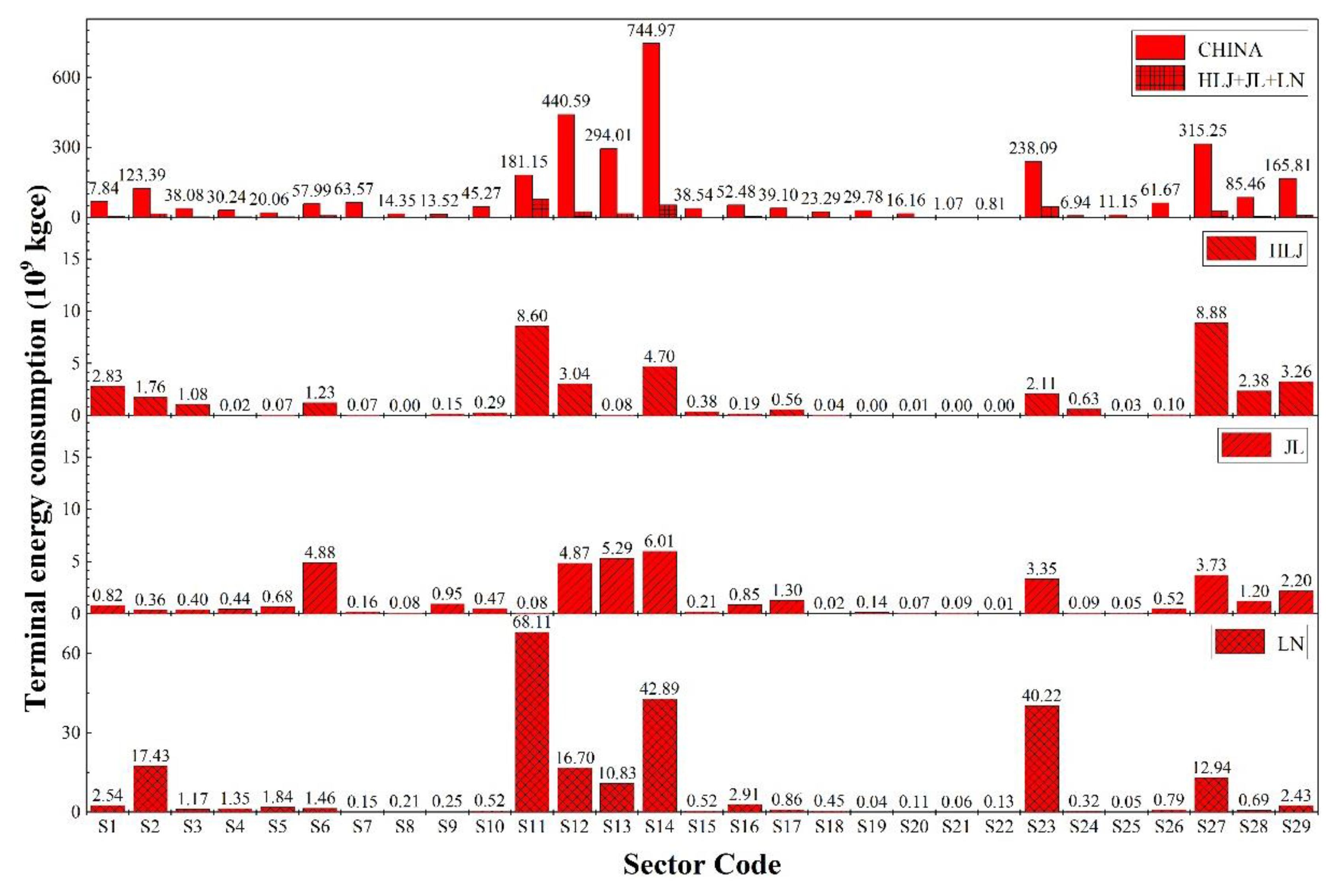
3.1. Terminal Energy Consumption

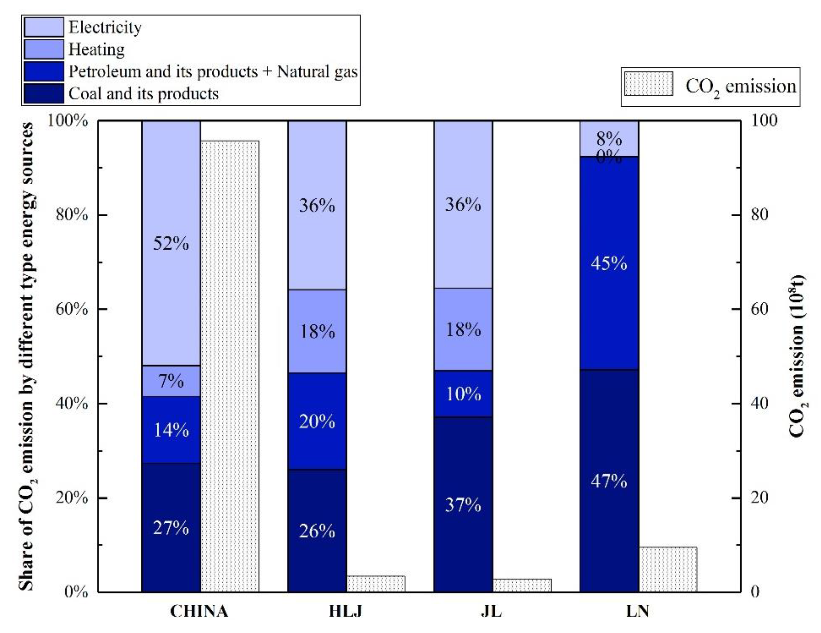
The total terminal energy consumption of China, HLJ, JL, and LN was 3220.66 million tons of coal equivalent (Mtce), 42.50 Mtec, 39.32 Mtec, and 222.67 Mtec, respectively, in 2012. The terminal energy consumption of HLJ, JL, and LN accounted for 1.32%, 1.22%, and 6.91% of that of China, respectively (Figure 2). From the sectoral perspective, smelting and calendaring of metals (S14) contributed the most to energy consumption in China, accounting for 23.13%, followed by manufacture of chemical products (S12) and transport, storage, and post (S27). However, the distribution characteristics of sectoral energy consumption of the three regions were different from that of China. The top three energy consumers were S14, petroleum processing and coking (S11), and S27 in HLJ (accounting for 52.18% of total energy consumption), S14, manufacture of non-metallic mineral products (S13), and manufacture of food and tobacco (S6) in JL (accounting for 41.14%), and S11, S14, and production and supply of heat and electricity (S23) in LN (accounting for 66.34%). The total energy consumption in LN was larger than the sum for HLJ and JL in 2012. Specifically, energy consumption of mining and washing of coal (S2), S11, S12, S13, S14, and S23 in LN was much larger than that of these sectors in HLJ and JL. According to the top panel in Figure 2, the sum of energy consumption of three regions in some sectors exceeded 1/10 of China’s corresponding sectors’, including high-energy-consumption sectors (mining and washing of coal (S2), manufacture of food and tobacco (S6), S11, and S23) and low-energy-consumption sectors (mining and processing of non-metal ores (S5), waste material (S21), repair services for metal products, machinery, and equipment (S22), and production and supply of gas (S24)). The above results show that the three heavy industrial regions were more energy-intensive, especially LN.

3.2. CO₂ Emissions

CO₂ emissions of HLJ, JL, and LN accounted for 3.58%, 2.94%, and 9.91% of that of China in 2012, respectively (Figure 3). Heat used by LN was not listed separately in the terminal energy consumption table published by the Statistics Bureau of Liaoning. Therefore, the category structure of energy sources was different from that in the other two regions and China. CO₂ emissions from heat and electric consumption accounted for more than 50% of total energy-related CO₂ emissions in HLJ, LN, and China. The shares of CO₂ emissions from different types of energy sources in HLJ and JL were similar. However, the proportion of CO₂ emissions from consumption of “petroleum and its products + natural gas” in HLJ (20%) was higher than that in JL (10%). In particular, CO₂ emissions from using “petroleum and its products + natural gas” and “coal and its products” both contributed over 45% of the total CO₂ emissions in LN. It can be concluded that LN is a region highly dependent on fossil fuel to support industrial production activities. At the national level, the proportion of CO₂ emissions from fossil fuel used to produce electricity was much larger than that of the three regions. Therefore, there is great potential to optimize the terminal energy consumption structure.

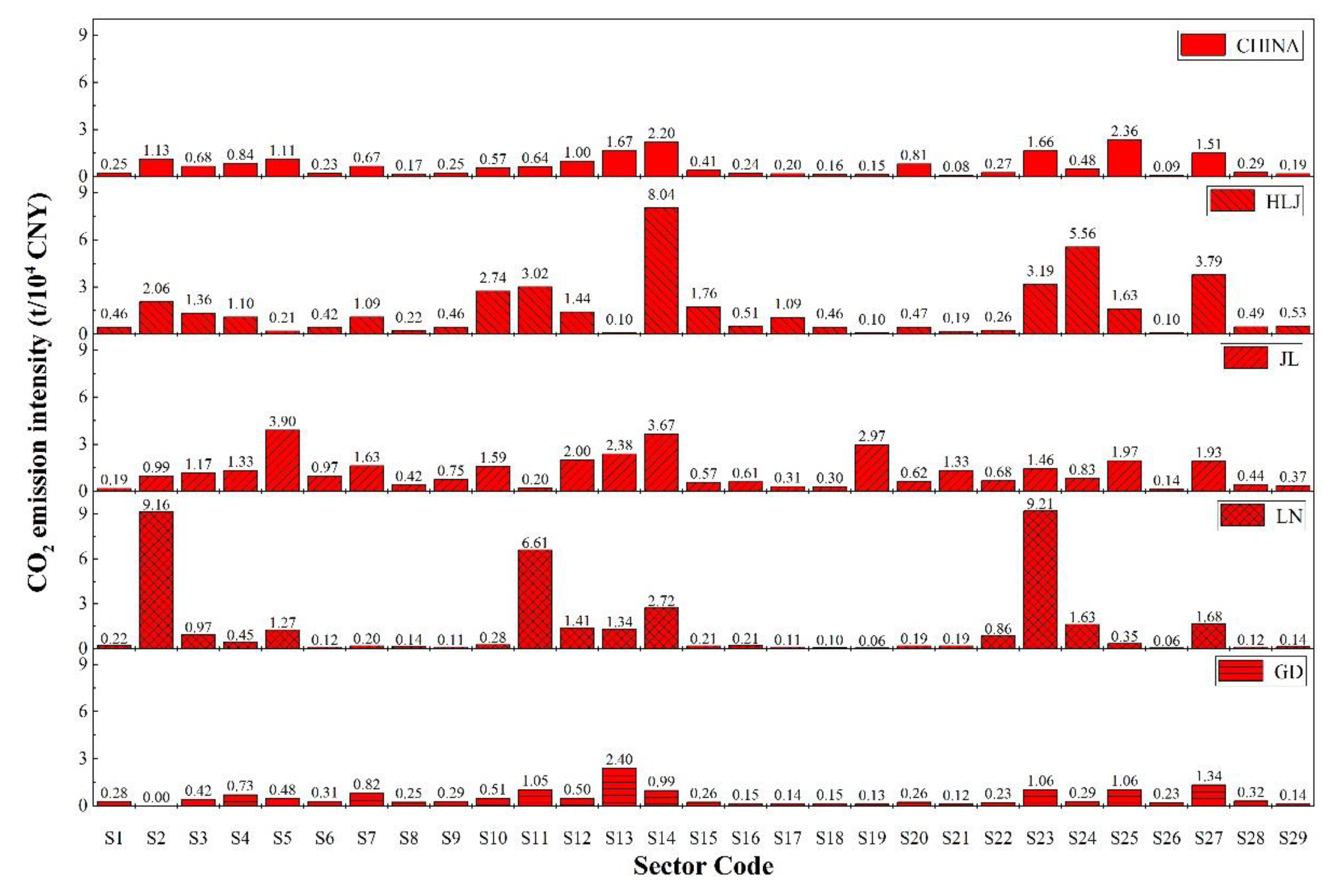
3.3. Sectoral CO₂ Emission Intensity

CO₂ emission intensity is defined as the amount of CO₂ emission of unit sectoral output. The sectoral CO₂ emission intensities of three regions and China in 2012 are shown in Figure 4. In order to investigate the differences in CO₂ emission intensity between heavy industrial and developed regions, we added Guangdong (GD) Province’s CO₂ emission intensity into Figure 4. The CO₂ emission intensities of HLJ, JL, LN, and GD were 1.85, 1.43, 2.00, and 0.68 times that of China, respectively. From the sectoral perspective, CO₂ emission intensities of S2, S11, and S23 in LN, S5 and S19 in JL, and S11, S14, and S24 in LN were much larger than that of China and GD. However, it is unreasonable to restrict the production of some sectors with relatively higher CO₂ emission intensity. This is because the sectors with high CO₂ emission intensity are usually recognized as critical sectors which provide raw material and energy to downstream sectors or supply products to final consumption sectors. Therefore, it is necessary to explore methods to balance the economic growth and CO₂ emission reduction.

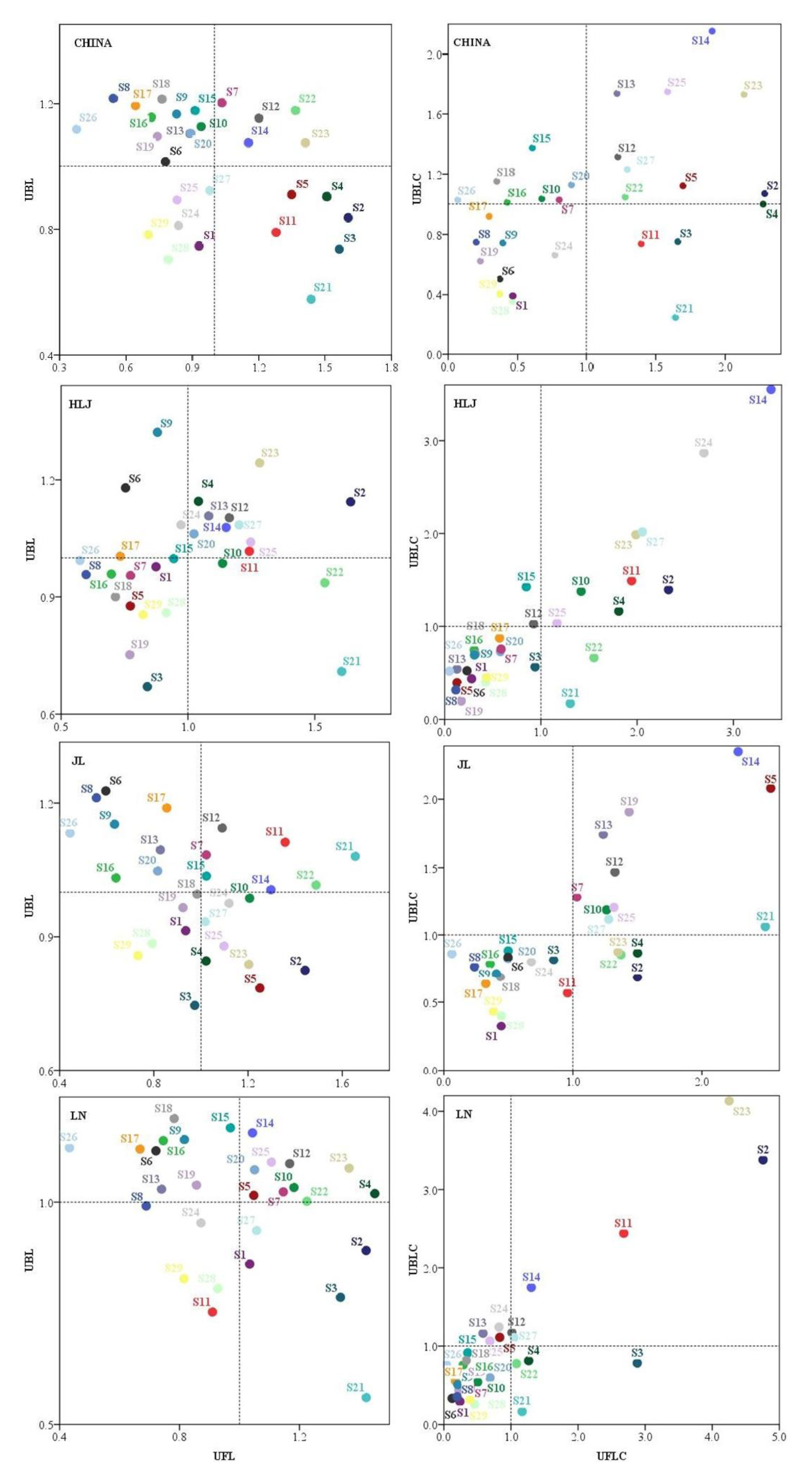
3.4. Sector–System Production and CO₂ Emission Linkages

The main goal of this study is to reduce carbon emissions while not affecting the economic growth obviously. It is clear that allocating the CO₂ emission reduction task by sector is unfair and unfeasible because all sectors are correlated in supply-and-demand relationships. Therefore, production limits should focus on industrial groups defined by linkage characteristics, rather than separate key emission sectors. Unified forward linkage of production (UFL), unified backward linkage of production (UBL), unified forward linkage of CO₂ (UFLC) emissions, and unified backward linkage of CO₂ (UBLC) emissions were quantified (see Equations (15)–(18)) to explore the effect of the unit change of one sector’s final demand or intermediate inputs on the entire economy and total CO₂ emissions. All panels are organized showing unified backward linkages on the vertical axis and unified forward linkages on the horizontal axis in Figure 5. Comparing the left and right panels, it can be clearly revealed that a unified linkage concept from economy into CO₂ emission terms increases the range of linkage values; this finding is consistent with Chang [27] and Lenzen [47]. The values of UFLC and UBLC (0.06–2.28 and 0.25–2.15 in China, 0.04–3.39 and 0.2–2.85 in HLJ, 0.06–2.49 and 0.32–2.36 in JL, and 0.03–4.76 and 0.17–4.13 in LN, respectively) distribute in a wider range than those of UFL and UBL (0.38–1.61 and 0.58–1.22 in China, 0.60–1.64 and 0.66–1.32 in HLJ, 0.44–1.66 and 0.75–1.23 in JL, and 0.43–1.45 and 0.56–1.19 in LN, respectively). From the perspective of the sectoral level, some specific sectors (i.e., S14 and S24 in HLJ, S14, S5, and S21 in JL, and S2 and S23 in LN) induce the wide distribution of linkage values in the three heavy industrial regions.

The definition of key sectors in terms of production and CO₂ emissions was explained in Section 2.3. For comparison, key productive sectors (left panels) and key CO₂ emission sectors (right panels) are identified in the upper right corner in each panel (see Figure 5). As an alternative way to reduce CO₂ emissions, industrial restructuring should be undertaken with sectoral groups as objectives, which corresponds to the values of unified forward and backward linkages of production and emission, simultaneously. If the sectors are non-significant sectors for production and key sectors for CO₂ emissions, they can be set as the constrained group ($UB{L}_j$ < 1, $UF{L}_i$ < 1, $UBL{C}_j$ > 1, and $UFL{C}_i$ > 1). If the sectors are key sectors for production and non-significant sectors for CO₂ emissions, they can be set as the encouraged group ($UB{L}_j$ > 1, $UF{L}_i$ > 1, $UBL{C}_j$ < 1, and $UFL{C}_i$ < 1). The productive change of encouraged sectors could affect the whole economy to a great extent and total CO₂ emission to a small extent. The productive change of constrained sectors would have the opposite effects. As shown in Figure 5, the encouraged sectors are S13 and other manufacturing industries (S20) for HLJ, S11 and manufacture of metal products (S15) for JL, and manufacture of paper and paper products; education and sport activities (S10), manufacture of textile (S7), and S20 for LN. When selecting the constrained sectors, we find that there were few sectors meeting the criteria. Thus, we lowered the production linkage criteria (values of UBL and UFL smaller than 1.2). The constrained sectors are S24 and S10 for HLJ, communication equipment, computer, and other electronic equipment (S19), S13, S25, S27, and S10 for JL, and S11 and S27 for LN.

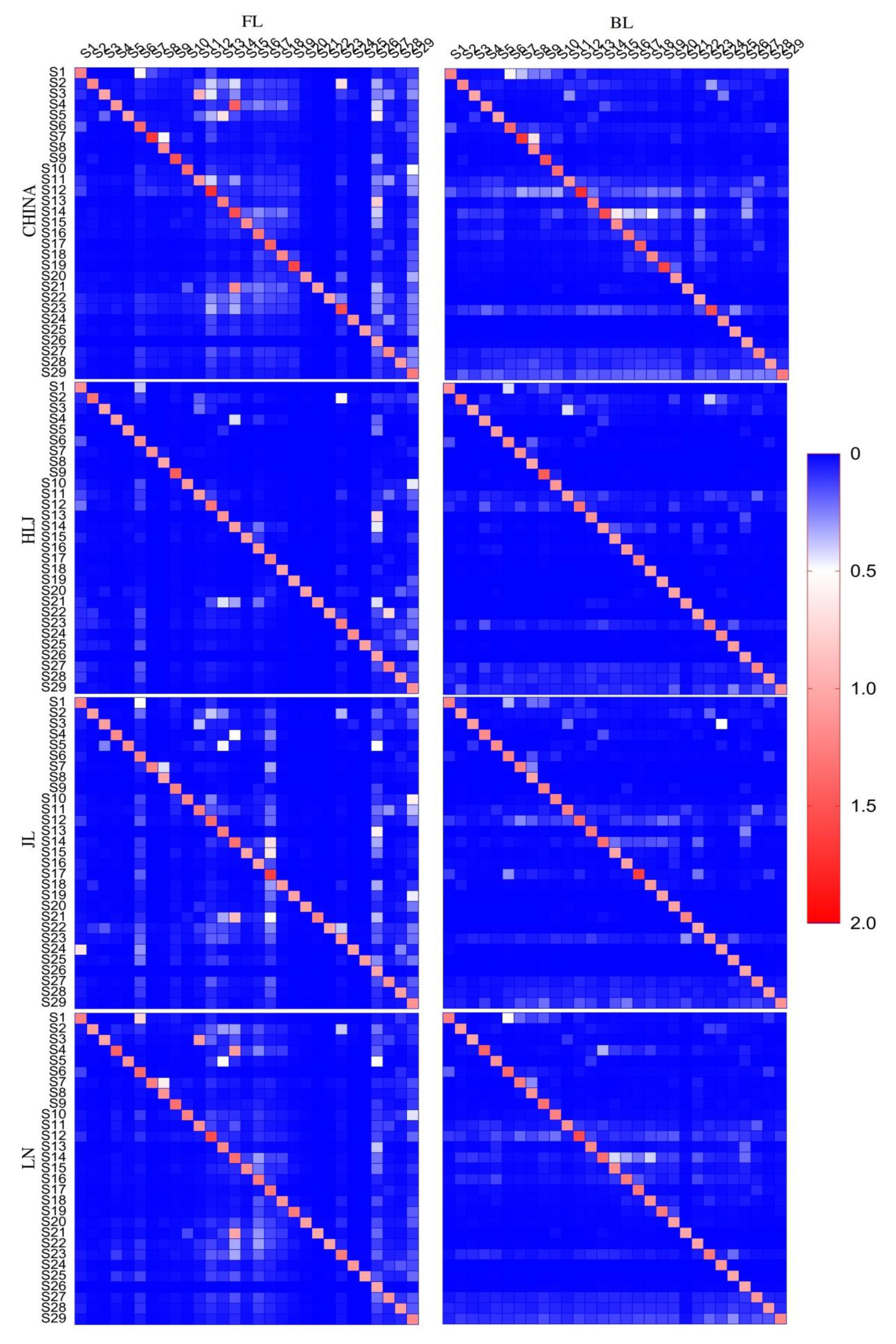
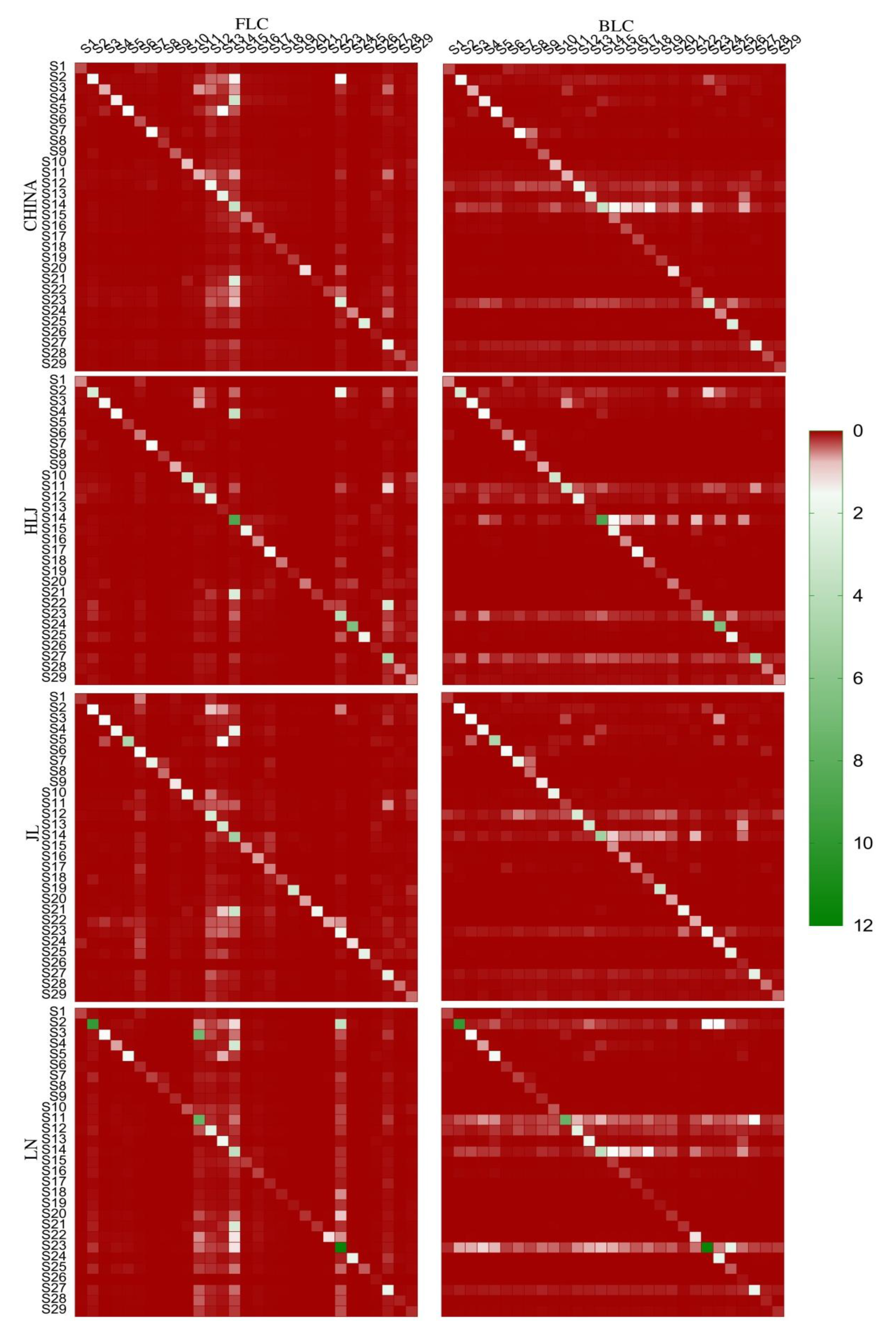
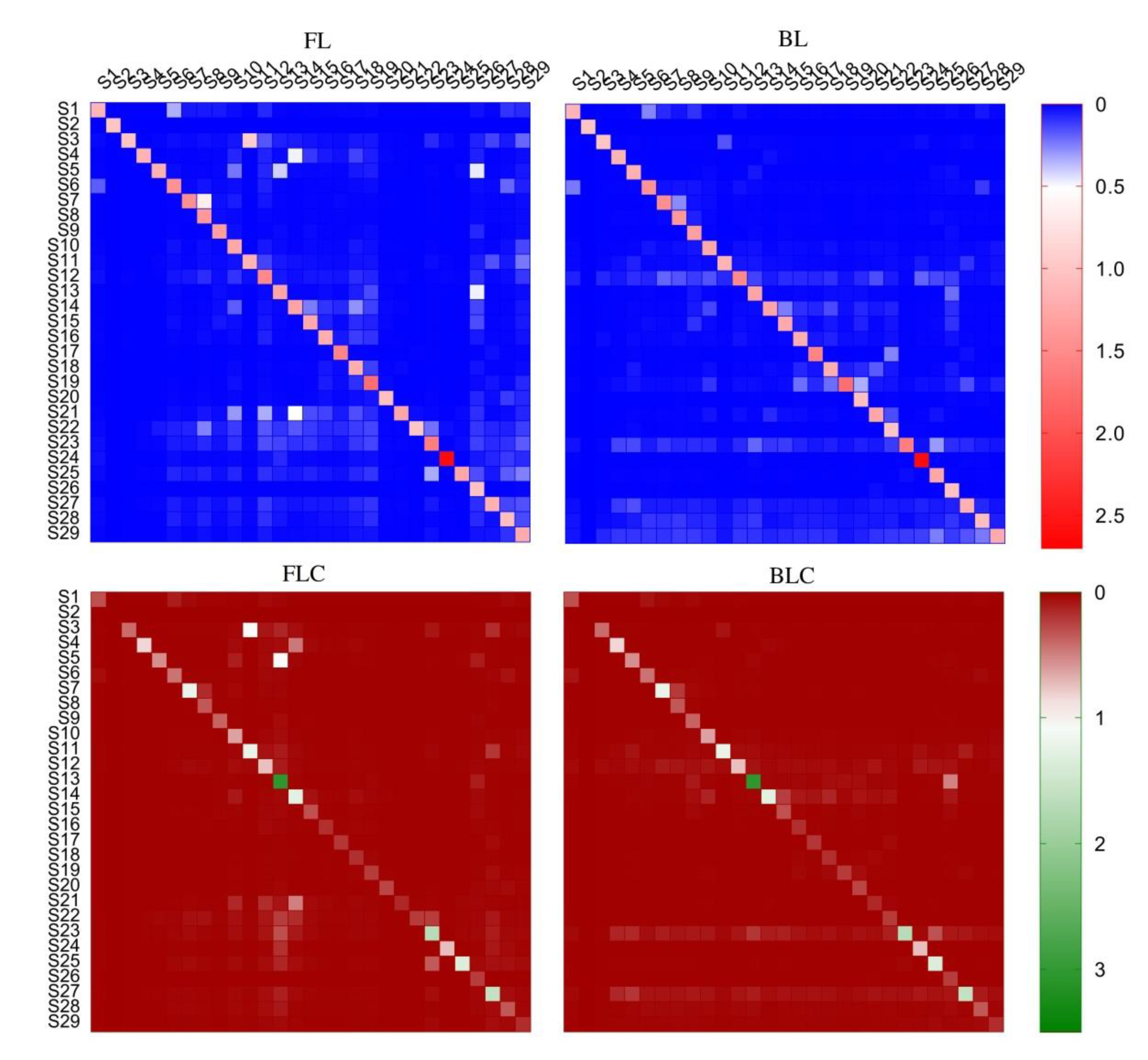
3.5. Sector–Sector Production and CO₂ Emissions Linkages

Section 3.4 helped to identify the encouraged and constrained sectoral groups. However, it is not sufficient to explore potential pathways toward energy-related carbon emission reduction. The pulling and pushing effects among sectors also should be well clarified, which can be accomplished by using sector–sector linkages. Backward linkage can quantify the extent to which a sector relies on other sectors for its inputs. Forward linkage can quantify the extent to which a sector supplies inputs to other sectors throughout the entire economy. The results of sector–sector linkages of production and CO₂ emissions are illustrated by Figure A2 and Figure A3 (see Appendix A), respectively. The sector–sector linkage results of GD (a developed region in China) (see Figure A4 in Appendix A) were also measured to clarify the gap between developed region and three heavy industrial regions.

HLJ’s sector–sector production linkages were weaker than those of GD or even JL and LN, with unobvious gaps among three heavy industrial regions. The structure features of sector–sector CO₂ emission linkages of the three heavy industrial regions were similar; however, they were far more complicated than that of GD. Specifically, the highest values of production and CO₂ emission linkages both occurred between one sector and itself (the main diagonal in each panel in Figure A2 and Figure A3, Appendix A). The reason for this phenomenon is that this study reorganized the sectors, and the aggregate sectors could be further divided into more detailed and closely related sectors in actual production activities. However, there were some exceptions; the largest values of FL/FLC occurred between mining and processing of metal ores (S4) and S14/waste material (S21) and S14 in China and JL; the highest values of FL and FLC occurred between extraction of petroleum and natural gas (S3) and S11 in HLJ and LN. The highest values of FL/FLC in the above three pairs of sectors represent the great pushing effect of the former sector on the latter sector. These special cases can be explained using actual production process; metal mining and manufacturing, waste and metal manufacturing, petroleum mining and processing are the adjacent sectors in the production chain with high energy consumption/carbon emission, respectively.

According to the FLC plots in Figure A3 (see Appendix A), some sectors in heavy industrial regions (S11, S14, S23, and transport, storage, and post (S27) in HLJ, manufacture of food and tobacco (S6), manufacture of chemical products (S12), manufacture of non-metallic mineral products (S13), S14, and manufacture of transport equipment (S17) in JL, and S2, S11, S12, S13, S14, S23, and S27 in LN) were intensively pushed by their upstream sectoral clusters to emit CO₂. According to the results, the high-energy-consumption sectors of HLJ and LN (e.g., metal mining and manufacturing, energy mining, and heavy industry) had a strong pushing effect on other sectors in terms of CO₂ emissions. JL is a major agricultural and vehicle manufacturing region, whose food-related industries and automobile industry have a great pushing effect on others in terms of CO₂ emissions. On the other hand, in the BLC plots, some sectors in heavy industrial regions (S2, S11, S12, S14, S23, and S27 in HLJ and LN, and S12, S14, S23, and S27 in JL) would pull upstream sectoral clusters to emit CO₂ to a great extent.

In HLJ and JL, for coal mining and chemical manufacturing, the BLC was larger than FLC. The reason is that the upstream sectors of these two sectors feature high energy consumption/carbon emissions. Thus, a unit increase in final demand of these two sectors’ products would drive more CO₂ emission from upstream sectors than that emitted by the downstream sectors pushed by a unit increase in intermediate inputs of these two sectors. On the contrary, in JL, food manufacturing and non-metallic mineral manufacturing industries had a great pushing effect on downstream sectors in terms of CO₂ emissions, whereas their pulling effect on upstream sectors (with relatively low CO₂ emission intensity) was lower in terms of CO₂ emissions. Attention should be paid to the differences between the above two situations. These sectors were all downstream sectors in the supply chain. The first case emphasizes the effect of other sectors on objective sector in terms of CO₂ emissions. However, the conditions for the second case are converse. For FL and BL, similar situations can be observed in the corresponding plots of each panel. We infer that this situation is mainly determined by the characteristics of the I–O structure of the three regions.

4. Discussion

4.1. Carbon Reduction Potential of Heavy Industrial Regions

The regional and national I–O tables are compiled every five years in China. The latest published I–O tables (2012) of the three heavy industrial regions and 2012 terminal energy consumption data were used in this study. In 2012, the use of terminal energy in heavy industrial regions (HLJ, JL, and LN) still mainly depended on fossil fuel. The proportion of renewable energy was lower than that of national level. Considering the sectoral production and energy-related CO₂ emissions, the backwardness of production technologies and the unsustainable energy structure in heavy industrial regions were more obvious, especially in HLJ and LN. From a sectoral perspective, most sectors in HLJ and LN have a large potential to reduce CO₂ emissions compared with the national level. Emphatically, MINING and washing of coal (S2), petroleum processing and coking (S11), and production and supply of heat and electricity (S23) should be focused on firstly due to their great potential for CO₂ emission reduction. Compared with HLJ and LN, the CO₂ emission intensity gap between JL and China was not so large. However, there was still a large gap between JL and a developed province (GD) in terms of CO₂ emission intensity.

4.2. Dividing Sectoral Clusters

For the three heavy industrial regions, the top three clusters in terms of CO₂ emission were S2 and S3 (mining and washing of coal; extraction of petroleum and natural gas), which provide the original resources and energy for downstream sectoral production; S11–S14 (petroleum processing and coking; manufacture of chemical products; manufacture of non-metallic mineral products; smelting and calendaring of metals), which provide critical materials to downstream manufacture sectors; and S27–S29 (wholesale and retail trades, hotels; catering services; other service sectors), which provide living goods/services to residents. However, it is difficult to obtain some clusters in terms of energy-related CO₂ emission intensity. In general, CO₂ emission intensities of production and supply of energy and resources industries (production and supply of heat and electricity (S23), mining and washing of coal (S2), and petroleum processing and coking (S11)) and heavy industries (S13, S14, and S5) are much higher than other sectors in the three regions studied.

However, if the industrial restructuring is conducted only based on sectoral terminal energy and sectoral CO₂ emission intensity, the macroeconomic benefit is lost to some extent. It must also be pointed out that allocating the emission reduction task by sector is unfair and unfeasible because all sectors are correlated in backward and forward partnerships. Therefore, to balance the conflict between CO₂ emission reduction and economic growth, production and CO₂ emission linkages should be jointly considered when discussing the role of sectors in an economy. Encouraged and constrained sectoral groups were established based on the sector–system linkages. The development of encouraged sectors can affect the whole economy to a great extent and slightly influence the total CO₂ emissions. Restricting constrained sector production can reduce total carbon emissions significantly with less impact on the whole economy. However, several sectors were classified into encouraged and constrained groups. Thus, based on the results of unified linkages of production and CO₂ emissions, we made a table as a key output ranking the sectors. In addition to encouraged and constrained sectors, slightly encouraged and constrained sectors were defined (see

Table A1. Classification of sectors in terms of potential of CO₂ emission reduction (UBL: unified backward linkage of production; UFL: unified forward linkage of production; UFLC: unified forward linkage of CO₂ emissions; UBLC: unified backward linkage of CO₂ emissions).

Sector Code	HLJ	JL	LN
S1
S2
S3
S4
S5
S6
S7
S8
S9
S10
S11
S12
S13
S14
S15
S16
S17
S18
S19
S20
S21
S22
S23
S24
S25
S26
S27
S28
S29

  : Encouraged sector ^a;   : slightly encouraged sector ^b.   : Slightly constrained sector ^c;   : constrained sector ^d. ^a Encouraged sector is determined by $UB{L}_j$ > 1, $UF{L}_i$ > 1, $UBL{C}_j$ < 1 and $UFL{C}_i$ < 1. ^b Slightly encouraged sector is determined by $UB{L}_j$ > 1, $UF{L}_i$ > 1, $UBL{C}_j$ > 1 and $UFL{C}_i$ < 1; $UB{L}_j$ > 1, $UF{L}_i$ > 1, $UBL{C}_j$ < 1 and $UFL{C}_i$ > 1; $UB{L}_j$ > 1, $UF{L}_i$ < 1, $UBL{C}_j$ < 1 and $UFL{C}_i$ < 1; $UB{L}_j$ < 1, $UF{L}_i$ > 1, $UBL{C}_j$ < 1 and $UFL{C}_i$ < 1. ^c Slightly constrained sector is determined by $UB{L}_j$ < 1, $UF{L}_i$ < 1, $UBL{C}_j$ > 1 and $UFL{C}_i$ < 1; $UB{L}_j$ < 1, $UF{L}_i$ < 1, $UBL{C}_j$ < 1 and $UFL{C}_i$ > 1; $UB{L}_j$ > 1, $UF{L}_i$ < 1, $UBL{C}_j$ > 1 and $UFL{C}_i$ > 1; $UB{L}_j$ < 1, $UF{L}_i$ > 1, $UBL{C}_j$ > 1 and $UFL{C}_i$ > 1. ^d Constrained sector is determined by $UB{L}_j$ < 1.2, $UF{L}_i$ < 1.2, $UBL{C}_j$ > 1 and $UFL{C}_i$ > 1.

, Appendix A). These results will help researchers and policy-makers to clarify the carbon reduction potential of each sector when formulating industrial restructuring.

4.3. Improvement Measures for Sectors

The non-competitive I–O model was used in this study; thus, the inflows from foreign countries and other regions in China (out-of-region) were removed. The four panels on the left in Figure A2 (Appendix A) show the intra-regional sectoral production linkage. The degree of the linkage is mainly affected by two factors: supply chain and the proportion of imports in output. Decreasing the value of the second factor decreases the value of UBL. For example, the proportions of imports in total output of manufacture of electrical machinery and equipment (S18) were 0.07, 0.73, 0.36, and 0.21 in China, HLJ, JL, and LN, respectively, and the S18 UBL values of China and three regions were 1.22, 0.90, 1.00, and 1.19, respectively. Of course, the impact of the second factor is much smaller than that of the first factor.

In Section 3.4, we pointed out the encouraged and constrained sectoral groups. For the encouraged sectors, the proportion in total output should be promoted [48]. We can take some measures to constrained sectors: optimizing the energy structure, increasing the share of renewable energy, improving energy efficiency through technological innovations, and reducing the proportion of constrained sectors’ output in total output [49,50]. However, according to the actual situation, the above approaches may not be all applicable. For example, the production of manufacture of non-metallic mineral products (S13) and transport, storage, and post (S27) in JL and S27 in LN should be restricted. However, according to Figure A2 (Appendix A), these three sectors have strong sector–sector linkage relationships with many sectors. Changing their production will induce unexpected turbulence in the economy. Therefore, for such sectors, some measures should be implemented for improving energy efficiency or changing the energy source. More specifically, as a heavy industry, S13 heavily relies on raw coal. Thus, it would be easier to improve energy efficiency than change the energy structure. However, S27 has a complicated energy structure. It would be easier to reduce carbon emissions by changing the energy structure [51].

5. Conclusions

Reducing CO₂ emissions by adjusting the industrial structure constrains the development of some sectors, which results in macroeconomic losses to some extent. In addition, allocation of emission reduction task by sector is unfeasible because all sectors are correlated in supply and demand relationships. For avoiding the above situations, we applied linkage analysis within the input–output framework to explore potential pathways toward energy-related carbon emission reduction in heavy industrial regions in China (Heilongjiang (HLJ), Jilin (JL), and Liaoning(LN)), considering the backward and forward partnerships among sectors. Sector–sector and sector–system linkages (forward and backward) of production and CO₂ emissions were quantified at regional (HLJ, JL, LN, and Guangdong (GD), a developed region) and national (China) levels. The encouraged and constrained sectoral groups in terms of CO₂ emissions were established. The significant findings are as follows:

A: The CO₂ emissions in HLJ, JL, and LN account for 3.58%, 2.94%, and 9.91% of that of China, respectively. The dependence on fossil fuel energy in the above three heavy industrial regions is higher than that in China.

B: Sector–system linkage analysis helped to identify the encouraged or constrained sectoral groups. Manufacture of non-metallic mineral products (S13) and other manufacturing industries (S20) in HLJ, other manufacturing industries (S11) and manufacture of metal products (S15) in JL, and manufacture of paper and paper products; education and sport activities (S10), manufacture of textile (S7), and S20 in LN were identified as encouraged sectors. Production and supply of gas (S24) and S10 in HLJ, manufacture of communication equipment, computer, and other electronic equipment (S19), S13, production and supply of water (S25), transport, storage and post (S27), and S10 in JL, and S11 and S27 in LN were suggested as constrained sectors. Based on the results obtained, four categories of sectors in terms of potential of CO₂ emission reduction were classified.

C: Some sectors set to be constrained have strong sector–sector linkage relationships with other sectors. Therefore, changing production of these sectors will induce unexpected turbulence in the economy. Improving energy efficiency, optimizing energy structure, and production technology innovations for these sectors should be considered with priority. In addition, the actual social situation and the sectoral practical significance should be included when formulating policies.

This study provides a potential pathway in heavy industrial regions toward energy-related carbon emission reduction. In the future, if more detailed data are available, we will carry out an optimization simulation to explore more details and practical results, which will help decision-makers to better formulate policies and measures.

References

1. Henson, S.A.; Beaulieu, C.; Ilyina, T.; John, J.G.; Long, M.; Séférian, R.; Tjiputra, J.; Sarmiento, J.L. Rapid emergence of climate change in environmental drivers of marine ecosystems. Nat. Commun. 2017, 8. [Google Scholar] [CrossRef] [PubMed]
2. Quadrelli, R.; Peterson, S. The energy-climate challenge: Recent trends in CO2 emissions from fuel combustion. Energy Policy 2007, 35, 5938–5952. [Google Scholar] [CrossRef]
3. Hansen, J.; Kharecha, P.; Sato, M.; Masson-Delmotte, V.; Ackerman, F.; Beerling, D.J.; Hearty, P.J.; Hoegh-Guldberg, O.; Hsu, S.L.; Parmesan, C.; et al. Assessing “dangerous climate change”: Required reduction of carbon emissions to protect young people, future generations and nature. PLoS ONE 2013, 8, e81648. [Google Scholar] [CrossRef] [PubMed] [Green Version]
4. General Office of the State Council, PRC. The 11th Five-Year-Plan of Energy Conservation and Emission Mitigation. 2010. Available online: http://www.gov.cn/zhengce/content/2010-05/05/content_4872.htm (accessed on 5 December 2019).
5. General Office of the State Council, PRC. The 12th Five-Year-Plan of Energy Conservation and Emission Mitigation. 2012. Available online: http://www.gov.cn/zhengce/content/2012-08/12/content_2728.htm (accessed on 5 December 2019).
6. General Office of the State Council, PRC. The 13th Five-Year-Plan of Energy Conservation and Emission Mitigation. 2017. Available online: http://www.gov.cn/zhengce/content/2017-01/05/content_5156789.htm (accessed on 5 December 2019).
7. Ouyang, Y.; Li, P. On the nexus of financial development, economic growth, and energy consumption in China: New perspective from a GMM panel VAR approach. Energy Econ. 2018, 71, 238–252. [Google Scholar] [CrossRef]
8. Yang, D.; Liu, B.; Ma, W.; Guo, Q.; Li, F.; Yang, D. Sectoral energy-carbon nexus and low-carbon policy alternatives: A case study of Ningbo, China. J. Clean. Prod. 2017, 156, 480–490. [Google Scholar] [CrossRef]
9. Shan, Y.; Liu, J.; Liu, Z.; Xu, X.; Shao, S.; Wang, P.; Guan, D. New provincial CO2 emission inventories in China based on apparent energy consumption data and updated emission factors. Appl. Energy 2016, 184, 742–750. [Google Scholar] [CrossRef] [Green Version]
10. Zhang, W.; Li, K.; Zhou, D.; Zhang, W.; Gao, H. Decomposition of intensity of energy-related CO2 emission in Chinese provinces using the LMDI method. Energy Policy 2016, 92, 369–381. [Google Scholar] [CrossRef]
11. Sun, Q.; Shi, K.; Damerell, P.; Whitham, C.; Yu, G.; Zou, C. Carbon dioxide and methane fluxes: Seasonal dynamics from inland riparian ecosystems, northeast China. Sci. Total Environ. 2013, 465, 48–55. [Google Scholar] [CrossRef]
12. Acs, Z.; Plummer, L.A.; Sutter, R. Penetrating the knowledge filter in “rust belt” economies. Ann. Reg. Sci. 2009, 43, 989–1012. [Google Scholar] [CrossRef] [Green Version]
13. Wang, C.; Wang, F.; Zhang, H.; Ye, Y.; Wu, Q.; Su, Y. Carbon Emissions Decomposition and Environmental Mitigation Policy Recommendations for Sustainable Development in Shandong Province. Sustainability 2014, 6, 8164–8179. [Google Scholar] [CrossRef] [Green Version]
14. Chinese Bureau of Statistics. China Energy Statistics Yearbook 2013; China Statistics Press: Beijing, China, 2013. (In Chinese)
15. Li, S.; Wang, S. Examining the effects of socioeconomic development on China’s carbon productivity: A panel data analysis. Sci. Total Environ. 2019, 659, 681–690. [Google Scholar] [CrossRef] [PubMed]
16. Leontief, W. Composite Commodities and the Problem of Index Numbers. Econ. Soc. 1936, 1, 39–59. [Google Scholar] [CrossRef]
17. Leontief, W. Environmental Repercussions and the Economic Structure: An Input-output Approach. Rev. Econ. Stat. 1970, 52, 262–271. [Google Scholar] [CrossRef]
18. Song, J.; Yang, W.; Wang, S.; Wang, X.; Higano, Y.; Fang, K. Exploring potential pathways towards fossil energy-related GHG emission peak prior to 2030 for China: An integrated input-output simulation model. J. Clean. Prod. 2018, 178, 688–702. [Google Scholar] [CrossRef]
19. Yang, W.; Song, J.; Wang, H.; Dong, L. Insights into variations and determinants of water pollutant discharge in Jilin, China: Investigations from multiple perspectives. J. Clean. Prod. 2019, 241, 118386. [Google Scholar] [CrossRef]
20. Li, L.; Zhang, J.; Tang, L. Sensitivity analysis of China’s energy-related CO2 emissions intensity for 2012 based on input-output Model. Proced. Comput. Sci. 2017, 122, 331–338. [Google Scholar] [CrossRef]
21. Su, B.; Ang, B.W.; Low, M. Input-output analysis of CO2 emissions embodied in trade and the driving forces: Processing and normal exports. Ecol. Econ. 2013, 88, 119–125. [Google Scholar] [CrossRef]
22. Su, B.; Ang, B.W.; Li, Y. Input-output and structural decomposition analysis of Singapore's carbon emissions. Energy Policy 2017, 105, 484–492. [Google Scholar] [CrossRef]
23. Hondo, H.; Sakai, S.; Tanno, S. Sensitivity analysis of total CO2 emission intensities estimated using an input-output table. Appl. Energy 2002, 72, 689–704. [Google Scholar] [CrossRef]
24. Butnar, I.; Llop, M. Structural decomposition analysis and input-output subsystems: Changes in CO2 emissions of Spanish service sectors (2000–2005). Ecol. Econ. 2011, 70, 2012–2019. [Google Scholar] [CrossRef]
25. Supasa, T.; Hsiau, S.; Lin, S.; Wongsapai, W.; Chang, K.; Wu, J. Sustainable energy and CO2 reduction policy in Thailand: An input-output approach from production- and consumption-based perspectives. Energy Sustain. Dev. 2017, 41, 36–48. [Google Scholar] [CrossRef]
26. Xu, X.; Mu, M.; Wang, Q. Recalculating CO2 emissions from the perspective of value-added trade: An input-output analysis of China’s trade data. Energy Policy 2017, 107, 158–166. [Google Scholar] [CrossRef]
27. Chang, N. Changing industrial structure to reduce carbon dioxide emissions: A Chinese application. J. Clean. Prod. 2015, 103, 40–48. [Google Scholar] [CrossRef]
28. Su, B.; Ang, B.W. Input-output analysis of CO2 emissions embodied in trade: The effects of spatial aggregation. Ecol. Econ. 2010, 70, 10–18. [Google Scholar] [CrossRef]
29. Wang, Z.; Yang, Y. Features and influencing factors of carbon emissions indicators in the perspective of residential consumption: Evidence from Beijing, China. Ecol. Indic. 2016, 61, 634–645. [Google Scholar] [CrossRef]
30. Wei, J.; Huang, K.; Yang, S.; Li, Y.; Hu, T.; Zhang, Y. Driving forces analysis of energy-related carbon dioxide (CO2) emissions in Beijing: An input-output structural decomposition analysis. J. Clean. Prod. 2017, 163, 58–68. [Google Scholar] [CrossRef]
31. Murakami, K.; Kaneko, S.; Dhakal, S.; Sharifi, A. Changes in per capita CO2 emissions of six large Japanese cities between 1980 and 2000: An analysis using “The Four System Boundaries” approach. Sustain. Cities Soc. 2020, 52, 101784. [Google Scholar] [CrossRef]
32. Li, J.; Huang, G.; Liu, L. Ecological network analysis for urban metabolism and carbon emissions based on input-output tables: A case study of Guangdong province. Ecol. Model. 2018, 383, 118–126. [Google Scholar] [CrossRef]
33. IPCC. 2006 IPCC Guidelines for National Greenhouse Gas Inventories, Prepared by the National Greenhouse Gas Inventories Programme; Eggleston, H.S., Buendia, L., Miwa, K., Ngara, T., Tanabe, K., Eds.; IGES: Kanagawa, Japan, 2006. [Google Scholar]
34. Simpson, D.; Tsukui, J. The Fundamental Structure of Input-output Tables, An International Comparison. Rev. Econ. Stat. 1965, 4, 434–446. [Google Scholar] [CrossRef]
35. Chen, G.Q.; Wu, X.F. Energy overview for globalized world economy: Source, supply chain and sink. Renew. Sustain. Energy Rev. 2017, 69, 735–749. [Google Scholar] [CrossRef]
36. Zhao, X.; Chen, B.; Yang, Z.F. National water footprint in an input-output framework-A case study of China 2002. Ecol. Model. 2009, 220, 245–253. [Google Scholar] [CrossRef]
37. Su, B.; Ang, B.W. Input-output analysis of CO2 emissions embodied in trade: Competitive versus non-competitive imports. Energy Policy 2013, 56, 83–87. [Google Scholar] [CrossRef]
38. Ghosh, A. Input-output approach in an allocation system. Economica 1958, 25, 58–64. [Google Scholar] [CrossRef]
39. Chinese Input-Output Association. Chinese Input-output Table 2012; China Statistics Press: Beijing, China, 2015. (In Chinese)
40. Statistics Bureau of Heilongjiang. Heilongjiang Input-Output Table 2012; China Statistics Press: Beijing, China, 2015. (In Chinese)
41. Statistics Bureau of Jilin. Jilin Input-Output Table 2012; China Statistics Press: Beijing, China, 2015. (In Chinese)
42. Statistics Bureau of Liaoning. Liaoning Input-Output Table 2012; China Statistics Press: Beijing, China, 2015. (In Chinese)
43. Statistics Bureau of Heilongjiang. Heilongjiang Statistical Yearbook 2013; China Statistics Press: Beijing, China, 2013. (In Chinese)
44. Statistics Bureau of Jilin. Jilin Statistical Yearbook 2013; China Statistics Press: Beijing, China, 2013. (In Chinese)
45. Statistics Bureau of Liaoning. Liaoning Statistical Yearbook 2013; China Statistics Press: Beijing, China, 2013. (In Chinese)
46. Lenzen, M. Aggregation versus disaggregation in Input-Output Analysis of the environment. Econ. Syst. Res. 2011, 1, 73–89. [Google Scholar] [CrossRef]
47. Lenzen, M. Environmentally important paths, linkages and key sectors in the Australian economy. Struct. Chang. Econ. Dyn. 2003, 14, 1–34. [Google Scholar] [CrossRef]
48. Li, Z.; Pan, L.; Fu, F.; Liu, P.; Ma, L.; Amorelli, A. China’s regional disparities in energy consumption: An input-output analysis. Energy 2014, 78, 426–438. [Google Scholar] [CrossRef]
49. Ang, B.W.; Pandiyan, G. Decomposition of energy-induced CO2 emissions in manufacturing. Energy Econ. 1997, 19, 363–374. [Google Scholar] [CrossRef]
50. Chen, W.; Lei, Y.; Wu, S.; Li, L. Opportunities for low-carbon socioeconomic transition during the revitalization of Northeast China: Insights from Heilongjiang province. Sci. Total Environ. 2019, 683, 380–388. [Google Scholar] [CrossRef]
51. Jiang, T.; Huang, S.; Yang, J. Structural carbon emissions from industry and energy systems in China: An input-output analysis. J. Clean. Prod. 2019, 240, 118116. [Google Scholar] [CrossRef]
Figure 1. Three typical heavy industrial regions of China.
Sustainability 12 02148 g001
Figure 2. Regional and national terminal energy consumption by sectors in 2012.
Sustainability 12 02148 g002
Figure 3. Regional and national total CO2 emissions and proportion contributed by different types of energy sources. Due to data unavailability on energy consumption for heating, the category structure of energy sources in Liaoning (LN) is different from that in Heilongjiang (HLJ), Jilin (JL), and China).
Sustainability 12 02148 g003
Figure 4. Regional and national CO2 emission intensity by sectors in 2012.
Sustainability 12 02148 g004
Figure 5. Sector–system unified linkages of production and CO2 emissions in China and three regions (UBL: unified backward linkage of production; UFL: unified forward linkage of production; UFLC: unified forward linkage of CO2 emissions; UBLC: unified backward linkage of CO2 emissions).
Sustainability 12 02148 g005