Joint Governance Regions and Major Prevention Periods of PM_2.5 Pollution in China Based on Wavelet Analysis and Concentration-Weighted Trajectory

Abstract

China has made some progress in controlling PM_2.5 (particulate matter with an aerodynamic diameter of ≤2.5 μm) pollution, but there are still some key areas that need further strengthening. Considering that excessive prevention and control efforts affect economic development, this paper combined an empirical orthogonal function, a continuous wavelet transform, and a concentration-weighted trajectory method to study joint regional governance during key pollution periods to provide suggestions for the efficient control of PM_2.5. The results from our panel of data of PM_2.5 in China from 2016 to 2018 could be decomposed into two modes. In the first mode, the pollution center was in central Shaanxi Province, and the main eruption period was from November to January of the following year. As the center of this region, Xi’an should cooperate with the four cities in eastern Sichuan (Nanchong, Guangan, Bazhong, and Dazhou) to control PM_2.5, since the eruption occurred in this area. Moreover, governance should last for at least two cycles, where one cycle is at least 23 days. The pollution center of the second mode was in the western part of Xinjiang. Therefore, after the prevention and control efforts during the first mode are completed, the regional city of Kashgar should continue to build a joint governance zone for PM_2.5 along the Tianshan mountains in the east, focusing on prevention and control over two cycles (where one cycle is 28 days).

1. Introduction

The occurrence of haze and severe PM_2.5 (particulate matter with an aerodynamic diameter of ≤2.5 μm) pollution has attracted broad attention around the world. Increased PM_2.5 concentrations lead to a deterioration in human health [1], visibility [2], the regional climate [3], and economic development [4], causing urgent environmental problems that need to be solved. Developing countries that are experiencing rapid urbanization suffer from severe PM_2.5 pollution, and their inhabitants are exposed to high PM_2.5 concentrations. In January 2013, China suffered the most severe haze weather in its history (since haze has been recorded). The concentration of PM_2.5 in the Beijing–Tianjin–Hebei region (the most polluted region in China) was as high as 500 μg·m^-3, which is much higher than the acceptable level of PM_2.5 concentrations (0–35 μg·m^-3) in China [5]: This caused widespread concern across China. In 2013, the Chinese State Council released an Atmosphere Pollution Prevention and Control Action Plan [6], which required that by 2017, the respirable particle concentration in prefecture-level cities should be at least 10% lower than 2012 concentrations; moreover, the number of days with good air quality should increase every year. To achieve this goal, local governments in China have taken multiple measures. However, the high pollution levels in this severely polluted region do not breed confidence. In the fourth quarter of 2018, there were still 27 cities with PM_2.5 concentrations above the “lightly polluted” level (75–115 μg·m^-3). Pollution control and the prevention of PM_2.5 still need further strengthening.

As for studies on PM_2.5 pollution, previous scholars have generally used descriptive statistical analyses and combined spatial autocorrelation analyses to study a spatial cluster of annual PM_2.5 concentrations [7,8,9]. However, concentrations change in space, which tends to change the means of local areas. In heavily polluted regions, PM_2.5 pollution is normally a superposition of pollutants from different sources. A quantitative analysis can only determine the overall distribution of PM_2.5 and the influencing factors of PM_2.5 pollution. When confronting a more specific situation, such as different pollution statuses in one polluted area or the pollution situation at different times on a shorter time scale, a metrology analysis is not suitable because short-term social and economic data are difficult to obtain: This also means that prevention recommendations are not possible.

The local control and prevention of pollution mainly focuses on the relocation of heavily polluted enterprises or on regulating cars. However, PM_2.5 pollution does not only come from local emissions, but is also influenced by meteorological conditions, such as wind direction and speed [10]. Local governments cannot mitigate pollution by themselves. Some common policies should be jointly developed by city governments in the most seriously polluted regions (instead of in traditional administrative regions) [11]. Considering the differences in PM_2.5 pollution levels and the characteristics of agglomeration, governments should implement differentiated regional pollution control strategies [7]: Prevention and control require cooperation [12]. Studies have already established hierarchical policies based on differentiated socioeconomic development conditions and requirements across Chinese cities [13,14]. Chen et al. [8] analyzed the socioeconomic factors of joint control using a geographically weighted regression method, establishing a strategy of joint control. Zhang et al. [15] built a PM_2.5 network correlation model to identify and demarcate regions with strong temporal intercorrelations using hourly PM_2.5 concentrations. These studies, however, have only analyzed the key aspects of joint control over PM_2.5 from the perspective of society and economics: They have not been focused on the sources of PM_2.5. PM_2.5 pollution is also closely related to atmospheric transportation. If heavily polluted regions could adopt joint control strategies for the sources of pollutants, the control of PM_2.5 would be more efficient.

Backward trajectory analysis is an important method for analyzing the sources of air pollution. Scholars have studied the regional transportation characteristics of atmospheric particles by analyzing their air mass trajectories [16,17,18,19]. Existing research has focused on descriptions of long-term pollution sources in a single region, which cannot distinguish between the air mass trajectory during a heavily polluted period and the air mass trajectory during a slightly polluted period. Considering that policies leading to PM_2.5 decreases in China have been implemented without taking economic costs into account (which might be unsustainable in the near future) [20], prevention should be primarily focused on heavily polluted periods in key regions to find a balance between the control of pollution and economic growth.

As for studies of polluted periods, previous researchers have mainly analyzed changes in PM_2.5 concentrations using statistical methods that include the year, quarter, or day to analyze variations in the concentration of PM_2.5 [7,9,15,21]. These researchers have used overall temporal information to analyze the evolutionary features of PM_2.5 based on a simple method, where temporal characteristics of PM_2.5 are evaluated with the assumption that the statistical properties of the time series do not vary over time. These types of studies can only uncover intense periods of high PM_2.5, ignoring the pollution cycle. Because of that, pertinent suggestions for control cannot be given. Meanwhile, PM_2.5 concentrations have a complex cyclical variation with several short and long periods, which makes it difficult to analyze the temporal changes in PM_2.5 concentrations. The wavelet transform method is a feasible and effective method for studying the laws of variation of air pollution time-series indexes [22]. Temporal variations are expressed well, and mutated signals of the PM_2.5 level can be identified through wavelet analysis [23]. Using the wavelet method, Chen et al. [24] discovered multiscale features that are indicated in the temporal evolution of PM_2.5. Huang et al. [25] used the wavelet transform method to obtain the characteristics of yearly changes and sudden changes in the PM_2.5 level. Liang et al. [26] utilized the wavelet approach to explore the potential association between PM_2.5 and influenza. In addition, the wavelet transform method is mainly used in PM_2.5 concentration predictions [27,28,29,30,31]. However, these studies have barely focused on the characteristics of periodic changes in the PM_2.5 concentration on a major scale.

The factors of time and space should both be considered in analyses of the period and location of heavy pollution. The empirical orthogonal function (EOF) method was originally introduced in meteorology as a method for extracting the dominant modes of spatial variability [32]: It has since been applied in climatological [33,34], hydrological [35,36], and geophysical studies [37]. This method can extract the main components of meteorological factors and temporal and spatial variations. This paper decomposes PM_2.5 concentrations and judges the pollution center through the PM_2.5 concentration distribution in different modes. Furthermore, it analyzes the counterpart time variation and cycle patterns, giving the foundation for an analysis of joint governance regions and control cycles.

Due to limitations with monitoring conditions, previous studies on the spatiotemporal distribution of PM_2.5 have mainly focused on the Yangtze River Delta [38], the Pearl River Delta [39,40], the Beijing–Tianjin–Hebei region [41], and other developed regions. Even if the scopes of these studies were national, pollutants in the western regions were characterized as missing or unpolluted due to missing data, which is not consistent with reality [7]. As the Chinese government has paid more attention to PM_2.5 issues, observation conditions across the country have improved. In 2013, there were only nearly 800 monitoring sites in the country [15], but as of December 2018, the number of sites exceeded 1600, covering the vast majority of the country. With these improvements in monitoring conditions, the pollution problem in the western region—which had not been studied before—has gradually come to light. Therefore, it is necessary to carry out a national PM_2.5 analysis of temporal and spatial variations according to existing conditions and to further expand previous research to create more accurate PM_2.5 studies in China.

First, this paper combines a spatiotemporal distribution of PM_2.5 with an analysis of the source of pollutants, studying the spatiotemporal distribution of PM_2.5 concentrations in China to identify seriously polluted areas and time coefficients. Moreover, we utilized a wavelet transform to analyze key pollution periods using time coefficients. Finally, a backward trajectory analysis and a concentration-weighted trajectory were utilized to study the joint prevention regions of seriously polluted areas at heavily polluted times, providing suggestions for the efficient control of PM_2.5. The main contributions of this work are summarized as follows:

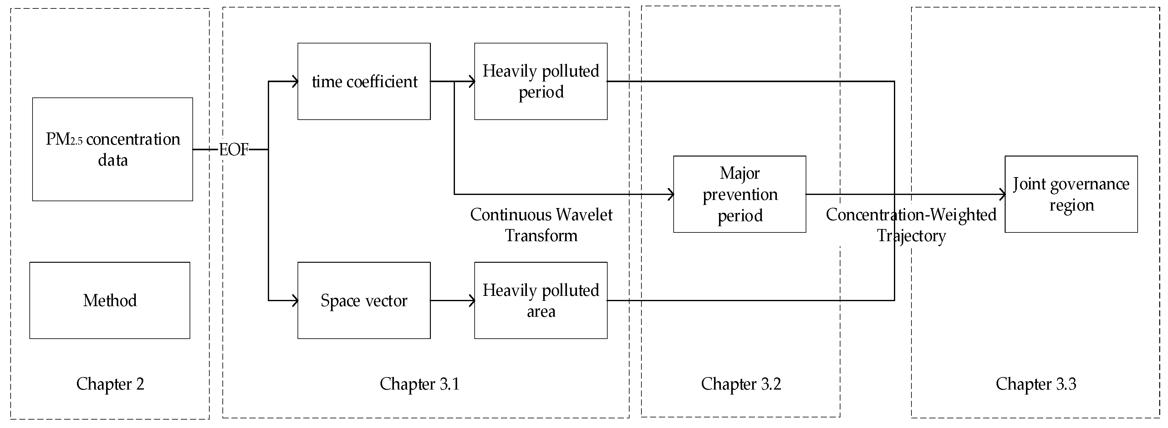
• The study of the spatiotemporal distribution of PM_2.5 concentrations. We applied EOF decomposition to the spatiotemporal distribution of PM_2.5 concentrations, studying the time coefficients and vectors of PM_2.5 concentrations in different modes and analyzing the overall average state and local variation of PM_2.5. Thus, regions and periods of heavy pollution could be determined.
• An analysis of the duration of key prevention and control strategies. The time coefficient of PM_2.5 concentrations under different modalities was analyzed using a wavelet transform to judge the length of time of serious pollution periods so as to provide suggestions for the duration of prevention and control policies.
• An investigation into the areas of joint protection and control. On the basis of the duration of key protection and control policies, PM_2.5 pollution in major cities in heavily polluted areas was analyzed using a backward trajectory analysis and a potential source analysis, with seriously polluted areas selected as the research object.

The rest of this paper is organized as follows (Figure 1): Chapter 2 describes our data sources and research methods. Chapter 3.1 presents a descriptive statistical analysis of the annual variation in PM_2.5 from 2016 to 2018, using EOF to decompose panel data of PM_2.5 concentrations to identify the periods of and areas with heavy pollution in different modes. Chapter 3.2 uses a continuous wavelet transform to analyze the duration of key protection and control policies. Using the above-mentioned pollution areas and prevention periods, Chapter 3.3 analyzes the joint prevention and control areas of the research object from the point of view of air mass trajectory. Chapter 4 is the conclusion.

2. Materials and Methods

2.1. Data Sources

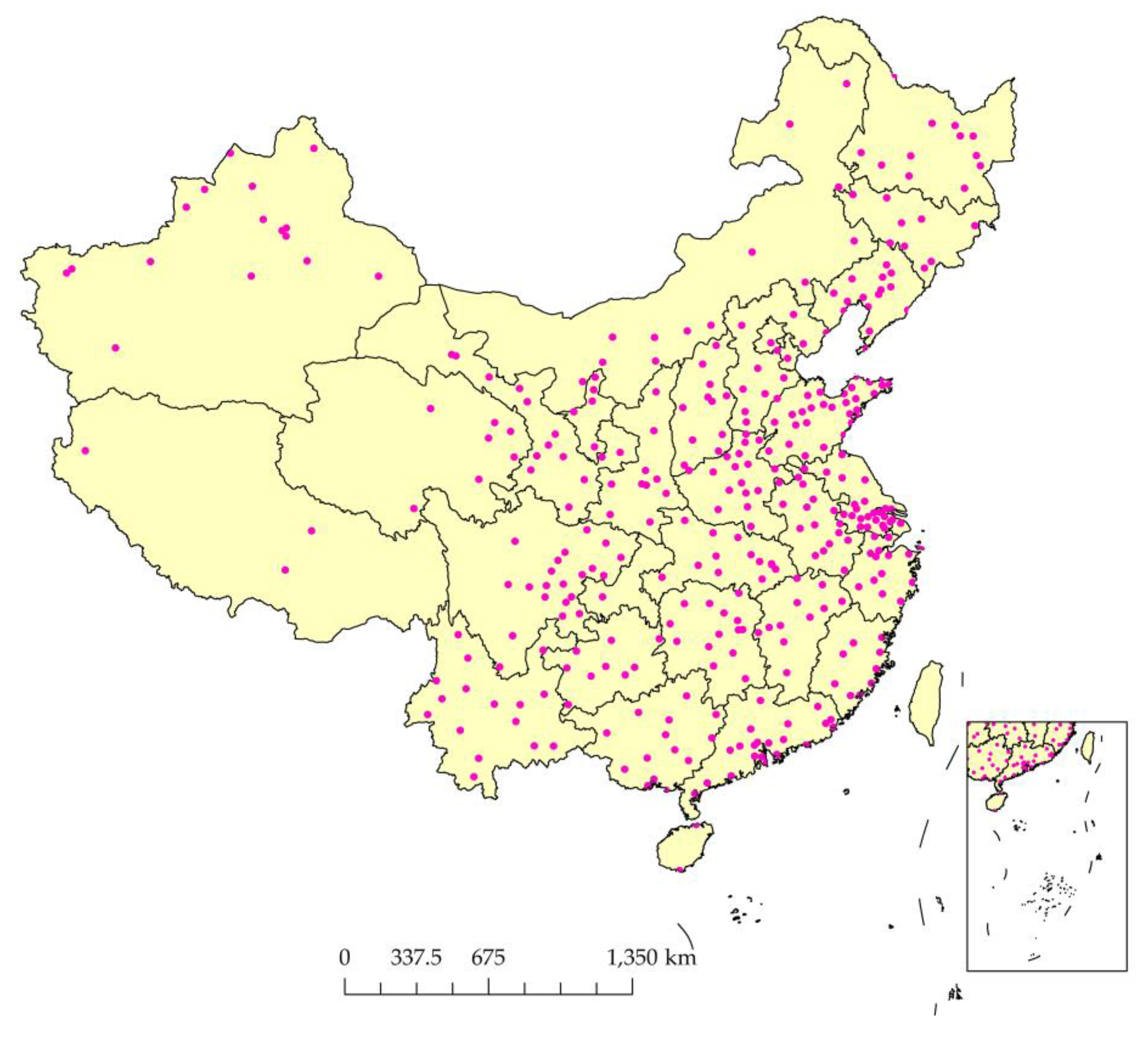
2.1.1. PM_2.5 Data

The PM_2.5 data were collected from the PM25.in website [42] (estimated by the National Urban Air Quality Real-Time Release Platform of China’s National Environmental Monitoring Center) [43]. The β-ray decay method and the tapered element oscillating microbalance (TEOM) method are commonly used as monitoring methods in China. Although these two methods are different in terms of measuring the concentration of PM_2.5 and although the TEOM is known to have seasonally dependent biases [44], there is no evidence that China’s ground monitoring data are not valid. Therefore, this paper used the (valid) ground monitoring data of PM_2.5 concentrations released by official data sources, which are widely used in academic research [8,15,24], without considering errors in the measurements.

This paper collected 24 h monitoring data from 361 cities in China, and daily and annual data were obtained through averaging. The positions of the selected cities are shown in Figure 2. An inverse distance weight algorithm [45] was employed to interpolate the PM_2.5 concentration and a simulation of the spatial distribution of pollution. The results, combined with geographic data, are presented in ArcGIS 10.2.

2.1.2. Backward Trajectory Analysis Data

The meteorological data, which were provided by the NCEP (National Environmental Forecasting Center), were exploited in backward trajectory mode (GDAS1 (Global Data Assimilation System) data). The meteorological element field included temperature, air pressure, relative humidity, ground precipitation, horizontal and vertical wind speed, etc., from 2016 to 2018. GADS1 has the capability of calculating trajectory directly using vertical wind speed, which is an advantage over other methods, whose vertical wind speed is calculated indirectly by calculating the vertical integration of horizontal wind speed divergence [46].

2.2. Method

2.2.1. Empirical Orthogonal Function

The empirical orthogonal function is a field analysis method widely used in the sphere of geosciences. Its principle is to decompose the spatiotemporal element field into several spatial basic modes and a linear combination of the time coefficient series, and then to objectively and quantitatively analyze the spatial structure and time changes of the element fields. The panel data of m observation points and n observations were expanded using the EOF and decomposed into the sum of the product of the orthogonal space matrix V and the orthogonal time matrix T:

$$X_{mn}=VT=\left(\begin{array}{ccc}{v}_{11}& \dots & v_{1n}\\ ⋮& \ddots & ⋮\\ v_{m1}& \cdots & v_{mn}\end{array}\right)\left(\begin{array}{ccc}{t}_{11}& \dots & t_{1n}\\ ⋮& \ddots & ⋮\\ t_{m1}& \cdots & t_{mn}\end{array}\right).$$

(1)

Equation (1) is multiplied on the right to get Equation (2):

$$X{X}^T=VT{T}^T{V}^T=V\Lambda V^T,$$

(2)

where the superscript T represents the transpose of the matrix, $\Lambda$ is a diagonal matrix composed of the eigenvalues of the matrix, and V is a matrix composed of the matrix eigenvectors.

Therefore, the time coefficient can be obtained from Equation (3):

$$T=V^{T}X.$$

(3)

North’s Rule of Thumb assesses the uniqueness of EOF modes through assumptions of error of the eigenvalues. When adjacent eigenvalues match the condition ${\lambda }_{j+1}-{\lambda }_j\ge {\lambda }_j{(\frac{2}{n})}^{\frac{1}{2}}$, these two eigenvalues and their corresponding modes pass the sampling error test [47].

The variance contribution rate ρ of the eigenvalues and the cumulative variance contribution rate of the first p eigenvalues are calculated as follows:

$${\rho }_i={\lambda }_i/{\displaystyle \sum _{i=1}^m{\lambda }_i},$$

(4)

$$p_i={\displaystyle \sum _{i=1}^p{\lambda }_i}/{\displaystyle \sum _{i=1}^m{\lambda }_i}.$$

(5)

In the EOF, a set of eigenvalues, eigenvectors, and time coefficients represents a distribution mode. The first few eigenvectors passing the significance test represent the maximum distribution structure. The component of the eigenvector with the largest absolute value represents the intensity center. If the positive and negative signs in the eigenvector are consistent, the eigenvector reflects the features with the same change trend. If the component of a certain eigenvector is in a positive and negative phase distribution, then this eigenvector represents two opposite distribution types. The time coefficient represents the time variation characteristics of the spatial distribution form. When the time coefficient is positive, the year is consistent with the distribution form represented by the eigenvector, and vice versa. The larger the absolute value of the time coefficient is, the more significant the distribution form. The variance contribution rate ρ reflects the degree to which a mode explains the whole. The higher its cumulative value is, the more accurately the selected mode describes the overall situation.

2.2.2. Continuous Wavelet Transform

A continuous wavelet transform can clearly reveal the period of change hidden in nonstationary time series and can reflect its change trend in different time scales. A continuous wavelet transform can also extract multiple wave periods from the wave sequence at different scales to reflect its changing trend, which is suitable for signal feature extraction [48]. The principle is to shift the mother wavelet function $\psi (t)$ after the translation $b$, and then to make an inner product with the signal $f(t)$ for it to be analyzed at different scales $a$, as follows:

$${\psi }_{ab}=\frac{1}{\sqrt{\left|a\right|}}\psi (\frac{t-b}{a}),$$

(6)

$$w_f(a,b)=\frac{1}{\sqrt{\left|a\right|}}{\displaystyle {\int }_{R}f(t)\overline{\psi }(\frac{t-b}{a})}\mathrm{d}t,$$

(7)

where $b=1,2,\dots ,N$. N is the number of datapoints (1096 in this paper). According to the literature [49], for nonorthogonal wavelet analyses, one can use an arbitrary set of scales $a$ to build a more complete picture. It is convenient to write the scales as fractional powers of two:

$$s_j=s_0{2}^{j\delta j},j=0,1\dots ,J,$$

(8)

$$J=\delta j^{-1}{\log }_2(N\delta t/s_0),$$

(9)

where $s_0$ is the smallest resolvable scale and $J$ determines the largest scale. Here, $\delta t$ represents the sampling intervals of data in this paper, and $s_0$ should be chosen so that the equivalent Fourier period is approximately $2\delta t$. For the Morlet wavelet, a $\delta j$ of about 0.5 is the largest value that can still give an adequate sampling scale. Parameter values from the literature [49] were used here: $\delta j$ = 0.125. Therefore, the smallest and largest resolvable scales could be calculated as 2 and 512, respectively. Note that longer scales correspond to the most stretched-out wavelets. The more stretched-out the wavelet is, the longer the portion of the signal to which it is being compared (and the coarser the signal features measured by the wavelet coefficients) will be. In addition, a large scale also means a long period. The time between the adjacent maximum and minimum of wavelet coefficients is almost 7 months when the scale $a$ is over 300 d (with similar data conditions) [24]. Because this article focuses on short-term trends in PM_2.5 concentration changes for efficient governance, the largest scale was set at 64, the same as in the literature [49].

The complex Morlet wavelet, which is a single-frequency complex sinusoidal function, which has symmetry, nonorthogonality, and an imaginary part [24], can simultaneously preserve the amplitude and phase information of the sequence signal of PM_2.5 concentrations. Therefore, a complex Morlet wavelet was selected as the mother wavelet. The complex Morlet wavelet function is as follows:

$$\psi (t)={(\pi \times f_b)}^{-0.5}{e}^{2i\times f_c\times t}{e}^{-t^2/f_b},$$

(10)

where t represents time and $f_b$ represents the bandwidth controlling attenuation in the time domain and the corresponding bandwidth in the frequency domain. Here, $f_b$ is the reciprocal of variance in the frequency domain. An increase in $f_b$ will lead to the wavelet energy being concentrated around the center frequency and will slow down the attenuation speed in the time domain. On the other hand, a decrease in $f_b$ will accelerate the decay rate in the time domain and reduce the energy of the frequency domain. Here, $f_c$ denotes the center frequency and affects the frequency value when the time domain is converted into a frequency domain [24,50]. These two parameters can be adjusted to obtain appropriate time–frequency resolutions. In this paper, we set the $f_b$ as 1 and the $f_c$ as 1.5, in accordance with parameter settings from the literature [24] and parameter optimization from the literature [51].

Using the MatlabR2018a software platform, the wavemenu toolbox was selected to calculate the wavelet coefficients. Meanwhile, the wavelet variance of the EOF time coefficient was analyzed to find the main scale. Then, the coefficient modulus of the wavelet coefficients and the contour plots of the real part were plotted to find the main oscillation periods and periods of time series at major scales. The periodic variation of the real part of the wavelet coefficient on the main scale was the most significant period of the time series.

A continuous wavelet transform can expand one-dimensional signals in both the time and frequency directions to analyze the time–frequency structure of the data in detail and extract valuable information. A continuous wavelet transform can not only provide the relative contribution of different scales of the time series, but can also indicate changes in different scales, so it is very helpful for the study of time series.

2.2.3. Backward Trajectory Analysis and Concentration-Weighted Trajectory

Here, we convey the calculation of the air trajectory first. The backward trajectory mode adopts the Hybrid Single-Particle Lagrangian Integrated Trajectory Model (HYSPLIT) developed by the NOAA (National Oceanic and Atmospheric Administration) [52,53]. The HYSPLIT model uses gridding meteorological data to respond to emergencies in the atmosphere to diagnose issues and analyze the climate. This mode is Lagrangian, as is Euler’s mixed diffusion mode: The processes of advection and diffusion are calculated using the Lagrangian method, and the concentration is calculated using the Euler Method [54]. HYSPLIT is considerably detailed in terms of the transportation, diffusion, and settling of pollutants, and its highest simulation accuracy can last hours. Thus, HYSPLIT is widely used in analyzing the source of pollutants and determining transmission and diffusion [55].

MeteoinfoMap is a geographic information system application that analyzes and visualizes multiple meteorological data formats [56]. Its plug-in, TrajStat, can use the backward trajectory analysis software adopted by the HYSPLIT Lagrangian diffusion module [57]. On the basis of the results from the EOF analysis, we selected cities with high pollution levels as the starting point and used the length of time of severe pollution as the pushback time. The air mass movement path at 500 m of altitude (the wind field at 500 m of altitude) can reflect the characteristics of the average flow field in the boundary layer [16,17,19]. Therefore, the height of the simulation was selected as 500 m, and we calculated the 48 h backward trajectory every 2 h.

After that, a grid was established based on the area covered by the atmospheric trajectory, with a resolution of 0.25° × 0.25°. The concentration-weighted trajectory (CWT) was used to analyze the source of pollution. The CWT is a mixed-trajectory receptor model that combines meteorological trajectory nodes (residence time) and pollutant concentrations to trace their contributions to the pollution of a recipient site [58]. After the study area was gridded, the CWT value of Grid (i, j) was as follows:

$$CW{T}_{ij}=\frac{1}{{\displaystyle \sum _{l=1}^M{\tau }_{ijl}}}{\displaystyle \sum _{l=1}^M{c}_l{\tau }_{ijl}},$$

(11)

where ${\tau }_{ijl}$ is the number of pollution trajectory nodes in the grid (i, j) in the area, and $C_l$ is the pollutant concentration of the trajectory. The higher the grid CWT value is, the greater the probability that the pollution trajectory comes from that grid point.

When there are fewer trajectories within the grid, the residence time is shorter, so the x value is higher and there is greater uncertainty. When $n_{ij}$ is less than three times its average value, we use the following weight function to reduce the uncertainty [58,59,60]:

$$WCW{T}_{ij}=W_{ij}\times CW{T}_{ij},$$

(12)

$$W_{ij}=\left\{\begin{array}{l}1.003n_{ave}<n_{ij}\\ 0.70n_{ave}<n_{ij}\le 3n_{ave}\\ 0.420.4n_{ave}<n_{ij}\le n_{ave}\\ 0.05n_{ij}\le 0.4n_{ave}\end{array}\right\}.$$

(13)

3. Results

3.1. Spatiotemporal Features of PM_2.5 Concentrations

3.3.1. Descriptive Statistical Analyses

According to the PM_2.5 concentration data from 2016 to 2018, the annual mean of the PM_2.5 concentration across the country had a downward trend. The national average PM_2.5 concentration value was reduced by a total of 6.753 μg·m^-3, representing 14.6% of the former value. The mean value decreased from 46.15 μg·m^-3 in 2016 to 43.76 μg·m^-3 in 2017, and then declined to 39.39 μg·m^-3. As is shown in Figure 3, except for the North China Plain, southern Sichuan, and part of western Xinjiang, the three-year average PM_2.5 concentration value in most areas was less than 55 μ·m^_3, which indicates good-quality air. In 2016, heavily polluted areas (in terms of PM_2.5 pollution) were mainly concentrated in western Xinjiang, the Beijing–Tianjin–Hebei region, Shanxi, Henan, central Hubei, central Shanxi, and west Shandong. In 2017, the concentration of PM_2.5 in the Shanxi, Anhui, Guangxi, Guangdong, Hainan, and Northern Xinjiang areas increased. At the same time, the PM_2.5 concentration in western Xinjiang dropped significantly. However, due to the high PM_2.5 concentration in western Xinjiang, although the decline was large, the air quality in Xinjiang was still worrying. Although PM_2.5 concentrations in most parts of the country were under control in 2018, PM_2.5 concentrations in western Xinjiang and Tibet continued to rebound slightly, and PM_2.5 concentrations also increased in western Yunnan and northern Gansu, indicating that in these areas, regional PM_2.5 prevention and control policies were not effective. These results differ from previous studies of the PM_2.5 distribution in China (by Hu Line [41]).

These research results should alarm the Chinese government: Although PM_2.5 has been under control in most regions of the country under current policies, PM_2.5 pollution remains a major problem in some regions. PM_2.5 concentrations did not always continue to decrease over the three years. Therefore, PM_2.5 prevention and control work should focus on these problem areas by strengthening control policies further, improving governance policies, and making PM_2.5 governance more effective.

3.3.2. Heavily Polluted Areas and Periods

In order to further understand the spatial and temporal distribution of PM_2.5 pollution and to accurately determine the key areas and periods of PM_2.5 governance, this paper used EOF analysis. We employed a standardized matrix of monthly panel data of PM_2.5 concentrations in 361 cities from 2016 to 2018. The characteristic vector of EOF expansion demonstrated the spatial distribution of the PM_2.5 concentration in each province. The maximum value center of all eigenvector fields indicated the region that was the most sensitive to PM_2.5 concentration changes. The eigenvectors of PM_2.5 concentrations in China’s provinces converged quickly, with eight eigenvalues passing North’s Rule of Thumb. The variance contribution rates of each mode were 41.70%, 10.77%, 6.56%, 4.72%, 3.63%, 2.93%, 2.12%, and 1.78%. The contribution rates of the eigenvalue variance illustrated that the EOF analysis results were ideal. Compared to the first two modes, the third mode and the subsequent modes took up a small proportion of the EOF decomposition. Therefore, the first two eigenvectors could be used to represent the spatiotemporal structure of PM_2.5 concentrations.

The variance contribution of the first mode of EOF indicated the average state of the PM_2.5 concentration from 2016 to 2018, representing the distribution field of PM_2.5 concentrations in China. In Figure 4, it can be seen that the first eigenvector had a consistently positive value, indicating that the spatial variation trend of PM_2.5 concentrations in the first mode was synchronous. The distribution pattern of the eigenvector in the first mode was close to the mean distribution (Figure 3a). It can be concluded that the first mode was the average state of PM_2.5 concentration. The highest value area was located in the middle of Shaanxi Province. The eigenvalues of North China, central Sichuan, and parts of Xinjiang were also large. This indicates that the PM_2.5 concentration fluctuated greatly in these areas. When the time coefficient was positive, PM_2.5 pollution was more severe. In other areas, the eigenvalue was close to zero regardless of changes in the time coefficient, so the PM_2.5 concentration remained at a low level.

From the distribution of the time coefficients in the first mode (Figure 5), it can be concluded that the PM_2.5 concentration change in the first mode had obvious seasonal characteristics. In the first and fourth quarters of each year, most PM_2.5 time coefficients were positive, and the maximum value each year appeared around December, which means that the high-value area of the eigenvector in the first and fourth quarters represented the PM_2.5 pollution problem getting worse and the pollution being the most serious from December to January. In the second and third quarters, the time coefficients were negative, so the PM_2.5 concentration gradually decreased. The dashed line in the figure is the linear regression of the time coefficients of the first mode, which had a downward trend, reflecting that in the long term, the pollution problems in the areas where the PM_2.5 concentrations changed after the first mode were alleviated.

According to the above analysis, in the first mode, the main pollution areas were Shaanxi, North China, Sichuan, and Xinjiang, and central Shaanxi. The main pollution periods were the first and fourth quarters of each year, and pollution was the most serious in December. Governments should focus on the above areas and pollution periods.

The second EOF mode reflected the spatial variation of regional PM_2.5 concentration differences; the spatiotemporal distributions are shown in Figure 6. Most of the eigenvalues exhibited in Figure 6 were close to zero, which meant that these regions contributed little to local pollution characteristics. However, the eigenvalues in Western Xinjiang had large negative values, suggesting dramatic changes in the PM_2.5 concentration.

It can be seen from Figure 7 that the time coefficients had large negative values from February to April each year, reaching a maximum on April 3, 2018. When looking at the eigenvectors of western Xinjiang in the second mode, in areas where the eigenvector is negative, negative time coefficients reflect a positive increase in the PM_2.5 concentration. The greater the absolute values of the time coefficients and eigenvalues are, the more severe the pollution is. It can be seen that the PM_2.5 pollution in the second mode was concentrated from February to April each year, and the pollution problem was extremely serious, especially in April (when there was an eruption of severe pollution). PM_2.5 governance in western Xinjiang should be strengthened during this period; the pollution problem in April is especially worthy of more attention.

3.2. Major Prevention Period

The PM_2.5 pollution periods in different modes were analyzed above. Local governments should focus primarily on severely polluted periods, especially in the western region of China, to strictly control PM_2.5 and further strengthen prevention and control efforts. However, considering the economic costs brought on by strengthening prevention and control efforts, the periods that are the most polluted should be of higher priority to be the most efficient. Since changes in PM_2.5 levels also have high-intensity periods, we suggest carrying out at least one complete control cycle for polluted periods. Prevention during heavily polluted times is key to helping improve control efficiency. Therefore, a wavelet transform was performed on the time coefficients in the two modes to further study what the best prevention time periods were.

The variance of wavelet transform coefficients can determine the main scale of the wavelet transform, which is plotted in Figure 8. The line chart represents the relative intensity of each scale in a time series. The scale at the corresponding peak is called the main time scale of the wavelet transform, and the periodic oscillation at this scale is the most significant. It is clear from Figure 8 that the wavelet variance of the time coefficients in the first mode had two distinct peaks corresponding to the time scales of 37 and 23 d. The periodic oscillation of the time scale around 37 d was the largest, which could mean that this is the main scale. In the second mode, the time scale of about 44 d had the largest variance.

The modulus value of the wavelet coefficient is a reflection of the distribution of the energy density at different time scales, which corresponds to the period of change in the time domain. The larger the modulus value of the coefficient is, the stronger the periodicity of the corresponding period or scale is. A contour map of the modulus of the wavelet variation coefficient is plotted in Figure 9. The red area in the figure indicates a large wavelet coefficient modulus value. The corresponding abscissa indicates a time of strong oscillation, and the ordinate is the wavelet transform scale. As can be seen in the figure, in the first mode, the strong period corresponding to the main scale (37 d) was from December 2017 to January 2018. The strongest period in the second mode was from February to March 2016 (at 44 d).

On the basis of the wavelet coefficient modulus and variance, the main scale of the time coefficient of changes in PM_2.5 concentration in the two modes (and their corresponding time range) was found. The main scale was used in the frequency domain analysis to determine the time domain change at different frequencies, which has no practical meaning. Because we wanted to focus on the most polluted periods from 2016 to 2018, we selected the scale with the largest variance of wavelet coefficients and the time range of the corresponding maximum value of the wavelet coefficient modulus. In practical applications, other typical scales or periods can also be selected for analysis according to actual needs, or all periods corresponding to the main scales can be selected for a comprehensive analysis. This method is very flexible.

A contour plot of the real part of the wavelet transform coefficient can reflect the change in the data at different transform scales. The ordinate of the densely arranged region at the center of the positive and negative values is the characteristic time scale of the wave sequence, and the abscissa is the periodic time frame of changes. In Figure 10, there are four red and blue local oscillation regions in the first mode and two local oscillation regions in the second mode. The two types of oscillations at different scales reflect different periodic changes. Each time the regions alternate between red and blue is a pollution period. The above analysis was carried out by selecting areas located in the main time scale and within the strong oscillating periods. The first mode (Figure 10a, the 37 d scale) experienced two pronounced concentration bursts between December 2017 and January 2018. In the second mode (Figure 10b), the cold- and warm-colored alternation regions were mainly concentrated in the period between February and April in 2016, with two cycles of strength and weakness on a 44 d scale. It is worth noting that there was a slight increase in the concentration of PM_2.5 before the eruption of the two modes, which indicates the beginning of a serious eruption of PM_2.5 pollution, an important early warning sign for PM_2.5 prevention. After the second eruption, the PM_2.5 concentration decreased to normal levels, and we defined the end of the second eruption as the end time of major pollution.

The above analysis determined the main scales, strong oscillation periods, and cyclic changes in the corresponding time coefficients. For the purpose of determining the PM_2.5 pollution cycle in different modes, the real part of the wavelet transform coefficients of different modes (with their main scales) was drawn. A typical polluted period was calculated using the intervals between the PM_2.5 concentration peaks. In Figure 11, the peak is the eruption time, the start is the short eruption time before the intense eruption of pollution, and the end is the ending time of the major pollution period. With these calculations, we could find out that the typical pollution time under the first mode was between 27 November 2017 and 26 January 2018, the outbreak interval was 23 days, and there were two intense pollution eruptions of PM_2.5. Pollution in the second mode occurred between 27 January 2016 and 31 March 2016, the outbreak interval was 28 days, and there were two intense pollution eruptions of PM_2.5 here as well.

Autocorrelation was used to verify the wavelet transform results. The autocorrelation results from the first and second modes’ time coefficients are shown in Figure A1 and Figure A2, respectively. According to the literature [61,62], the time differences between peaks can be calculated—we did that here to find that there existed a long period of 22 days, a result very close to the wavelet transform results from the first mode. Though the autocorrelation of the second mode was weaker than that of the first mode, a long period of 25 days was found for the time coefficient of the second mode, which was only a three-day difference compared to the wavelet analysis results. The autocorrelation results certified that the continuous wavelet transform method could find periods of time series from weak autocorrelation and can be used reliably in PM_2.5 concentration research.

On the basis of the above results, Shaanxi, northern China, Sichuan, and some parts of Xinjiang (whose PM_2.5 performances were poor during the first mode) should commence their governance between November and January of the following year (when PM_2.5 pollution is severe). The governance in these regions should last for two cycles after slight PM_2.5 pollution occurs for the first time, and one cycle should last for no less than 23 days. Governance in western Xinjiang should be strengthened in terms of prevention and control (in the first mode) until March. There should be at least two cycles during this period, and one cycle should last for 28 days.

3.3. Joint Governance Region

On the basis of the analysis above, we selected the cities of Xi’an and Kashgar for analysis. Both cities were in the most polluted areas in both modes. Taking the most severely polluted period as the calculation time, we used a backward trajectory of 48 h to analyze the major joint-governance cities. The backward trajectory analysis and concentration-weighted trajectory conditions are shown in

Table 1. The backward trajectory analysis and concentration-weighted trajectory conditions.

	Location	Start Time	End Time	Calculated Time	Grid Area
1	Xi’an (34.27°N, 108.93°E)	2017.12.3	2018.1.26	55 days	28.00°N~53.00°N, 73.00°E~120.00°E
2	Kashgar (39.47°N, 75.98°E)	2016.1.27	2016.3.31	65 days	30.00°N~50.00°N, 50.00°E~89.00°E

.

Here, the atmospheric trajectory image and CWT values reflect the effect of grid points on the PM_2.5 levels of the analyzed city. The larger the grid value is, the more serious the impact of PM_2.5 pollution on the city. In order to better identify major pollution sources, only high-value CWT grids in China are plotted, which are shown in Figure 12 and Figure 13. The CWT diagram of all grids is shown in Figure A3 and Figure A4.

In Figure 12, it can be seen that Nanchong, Guangan, Bazhong, and Dazhou in the eastern Sichuan Province had the greatest impact on PM_2.5 pollution in Xi’an. During the most polluted winter, PM_2.5 in eastern Sichuan passed through Ankang, Hanzhong, and Shangluo in southern Shaanxi Province and reached Xi’an, exacerbating PM_2.5 pollution. In addition, Weinan, Yanan, and Yuncheng in the northeast were also sources of PM_2.5 pollution in Xi’an. Therefore, prevention and control strategies in Xi’an should not be limited to local governance, and joint governance should be carried out between the above cities to control pollution more effectively.

The sources of severe pollution in Kashgar are shown in Figure 13. The PM_2.5 concentration in Kashgar was most influenced by the eastern region, which had heavy pollution. The grids of these trajectories were distributed along the Tianshan Mountains, starting from Bayingol and reaching Kashgar via Aksu, Aral, Tumshuk, and North Kashgar. Therefore, Kashgar should create prevention and control strategies for the urban agglomerations along the Tianshan Mountains.

4. Conclusions

This paper analyzed joint governance regions and key governing cycles in China through the EOF and backward trajectory analysis. The EOF decomposed PM_2.5 concentration panel data into space vectors and time coefficients. The time coefficients reflected the changing trends in pollution distribution. After transforming the time coefficients using wavelets, we could obtain the pollution periods of the main time scales and could determine key governance periods using the real parts of the wavelet coefficients. A space vector indicated the distribution of PM_2.5 pollution, which helped identify areas with serious pollution problems. Then, we selected the main cities in these areas and analyzed their sources of pollution during key governance periods to determine possible joint prevention areas. The conclusions can be summarized as follows:

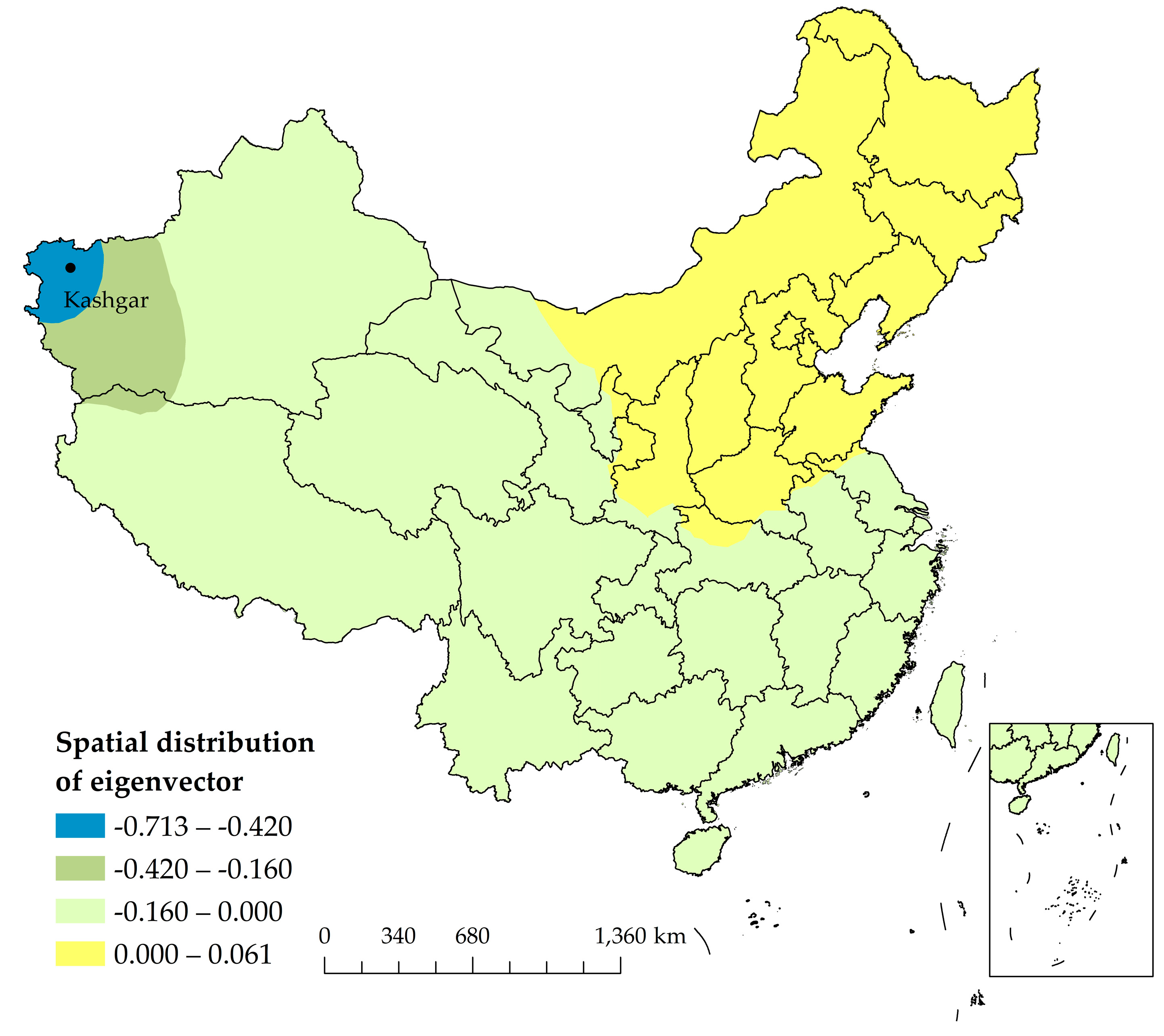
• From a nationwide point of view, the overall PM_2.5 pollution in China improved from 2016 to 2018, but the improvement was limited. PM_2.5 remains a serious problem in Xinjiang and North China. This finding is different from previous studies that have claimed that China’s PM_2.5 pollution is strong in the east and weak in the west. National PM_2.5 concentration panel data were decomposed using the EOF, resulting in two modes. The first mode reflected the average state of PM_2.5 pollution in China. Seriously polluted areas included northern China, western Sichuan, and parts of Xinjiang. The most polluted areas were in central Shaanxi Province. Pollution in the first mode had significant seasonal characteristics, indicating that pollution in the first and fourth quarters was serious and that the pollution degree decreased in the second and third quarters. The second mode reflected the local pollution characteristics of the Xinjiang region, indicating that there was severe pollution from February to April.
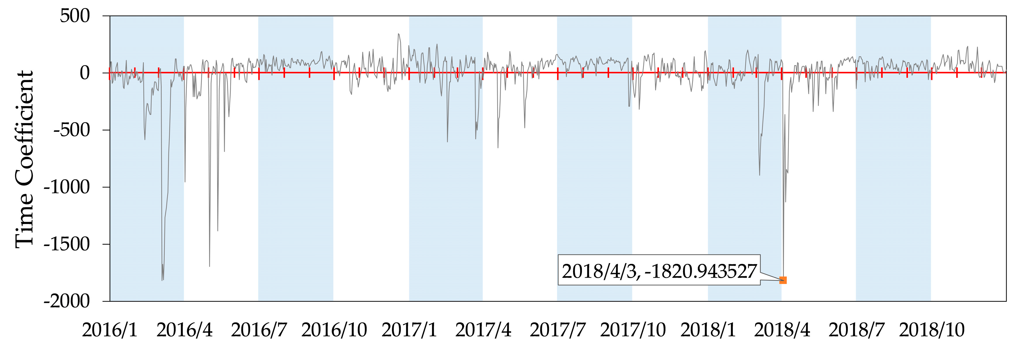
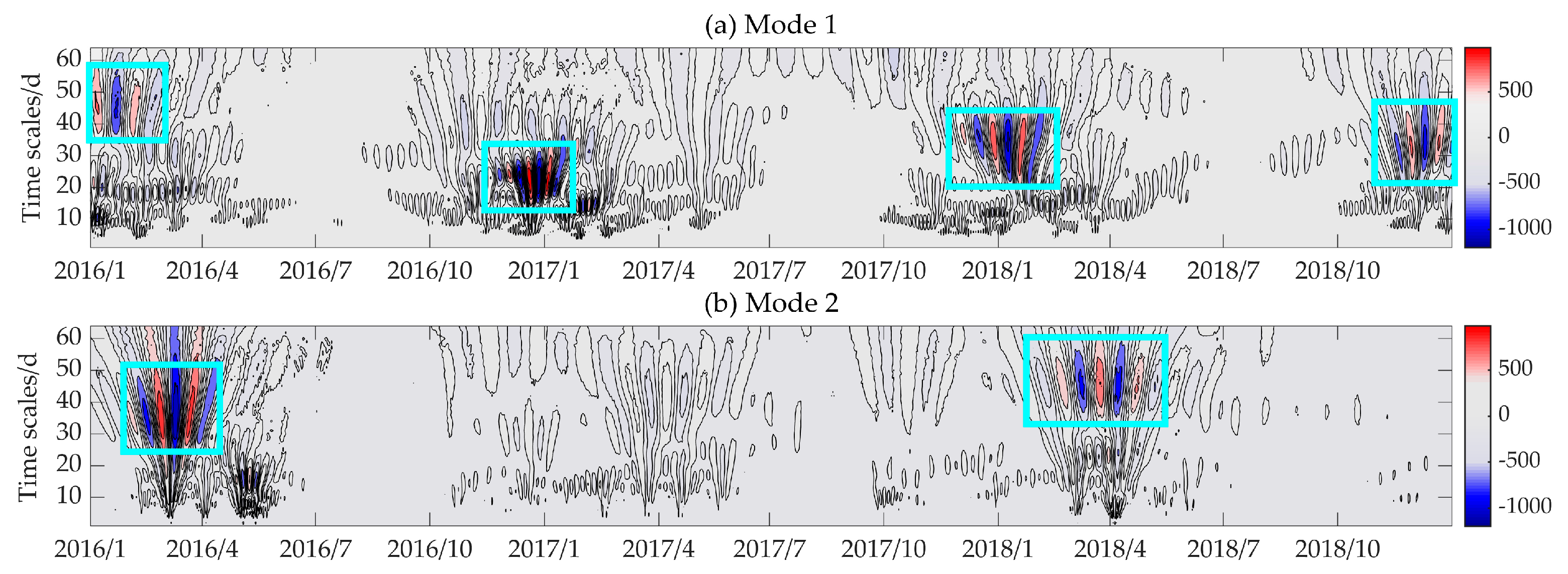
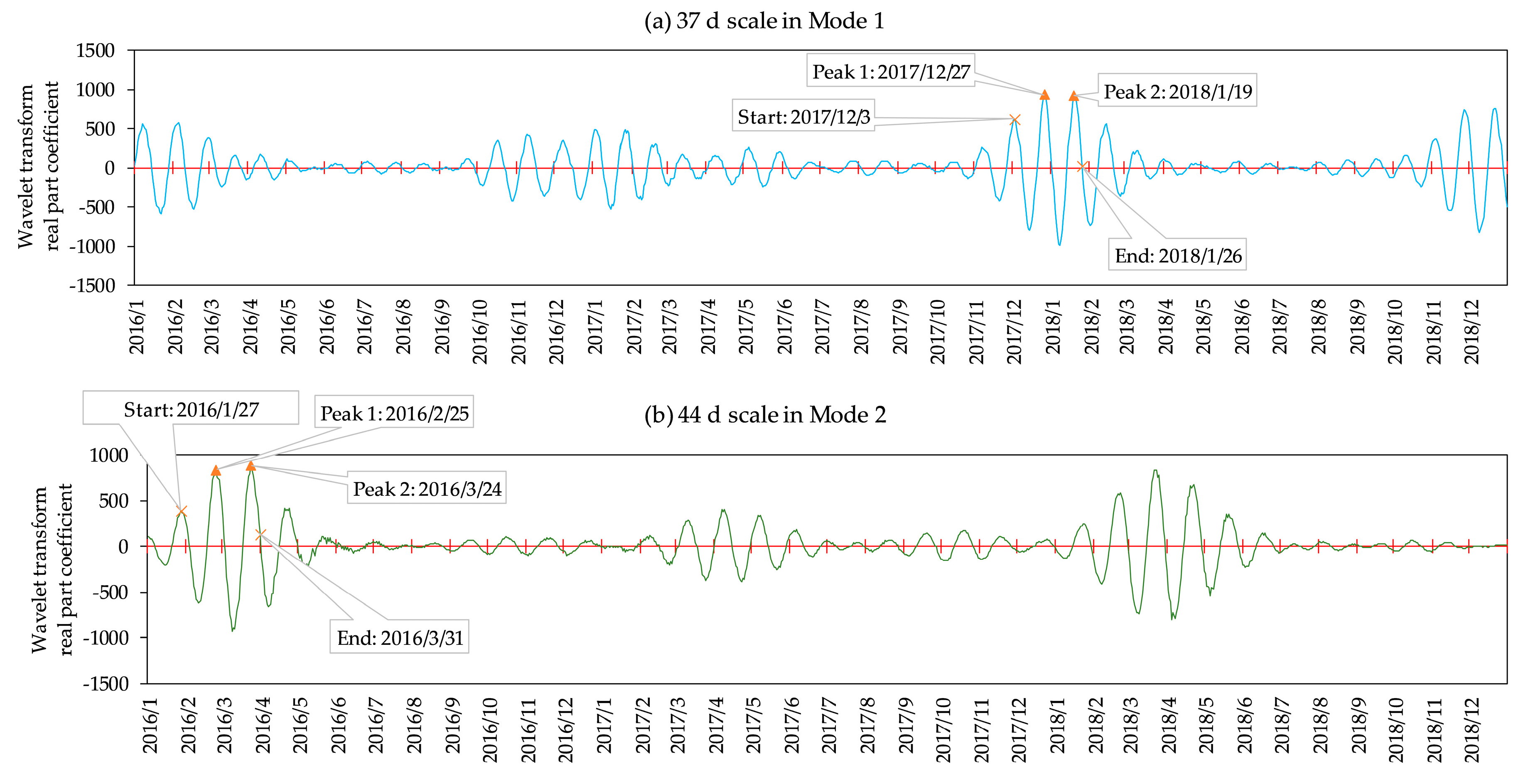
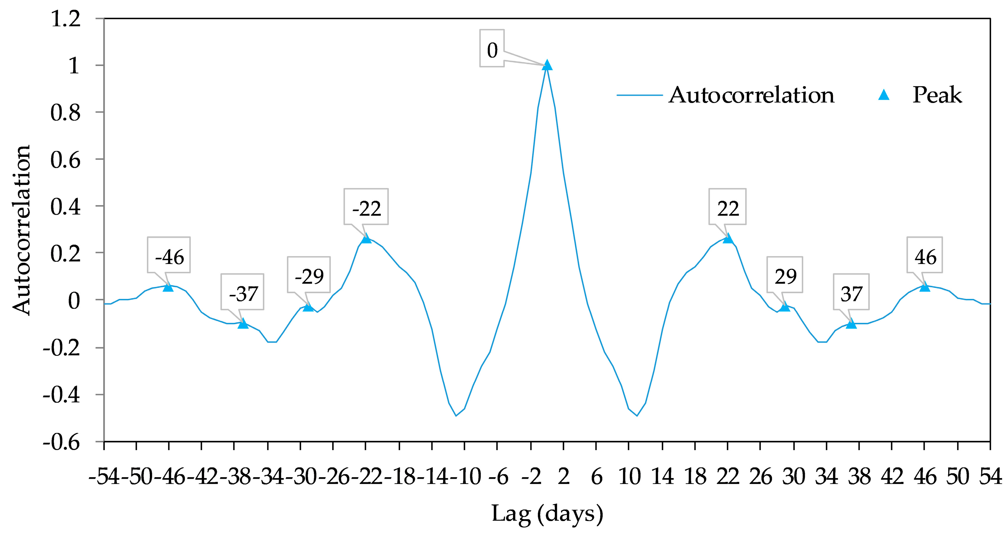
• Major prevention periods during the two EOF modes were studied using a continuous wavelet transform. This showed that the first mode had a typical oscillation, with a scale of 37 d, from November to January of the following year, and the main oscillation scale of the second mode was 44 d, from February 2016 to April 2016. In the areas where PM_2.5 pollution was in the first mode, prevention and control strategies should be carried out from November to January of the following year. After a small eruption in pollution occurs, prevention and control should be implemented for a period of no less than 23 days. After the end of the control cycle in the first mode, management and control of PM_2.5 pollution in the second mode should be strengthened for at least two cycles until March, where one cycle is 28 days.
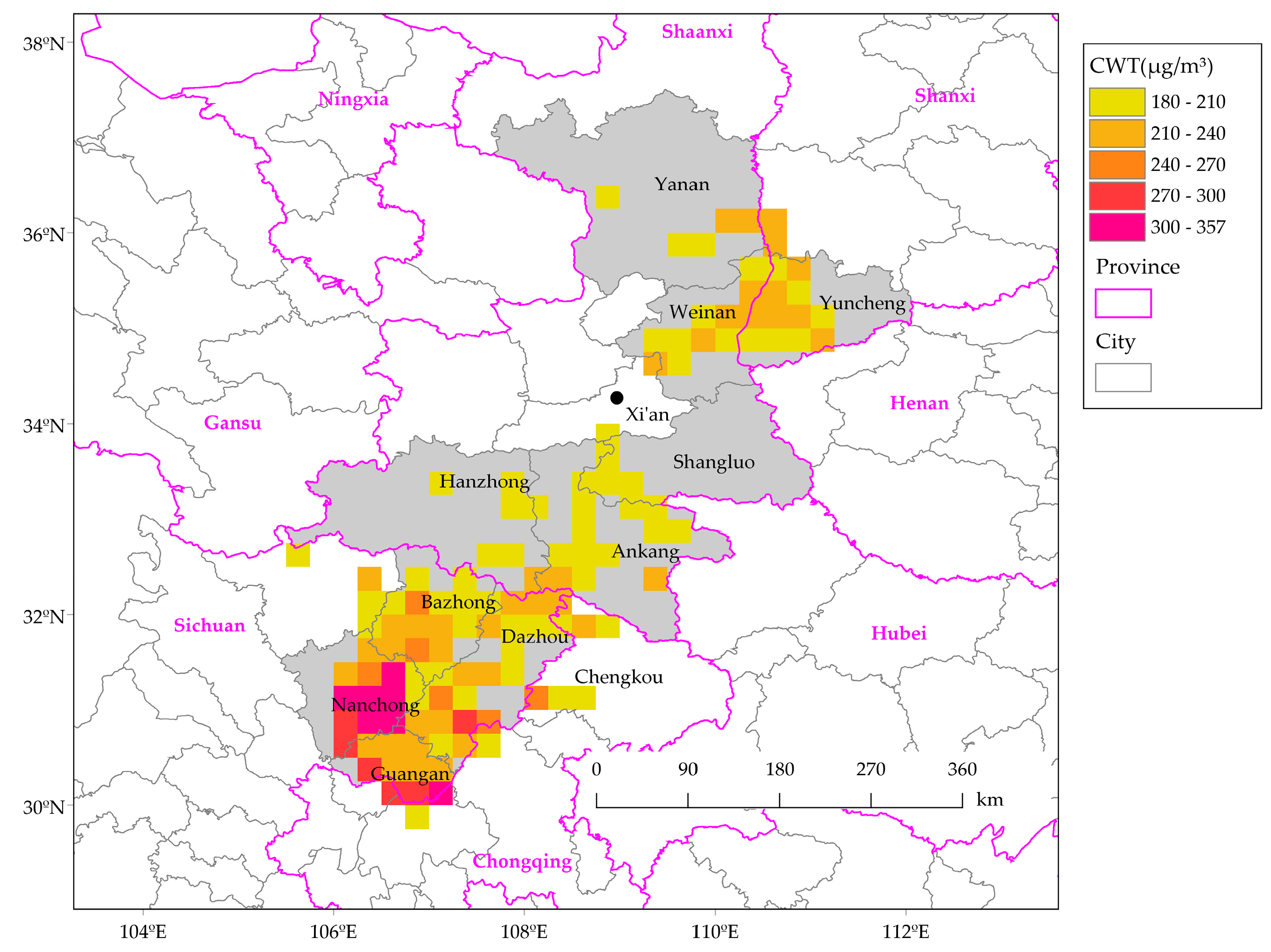
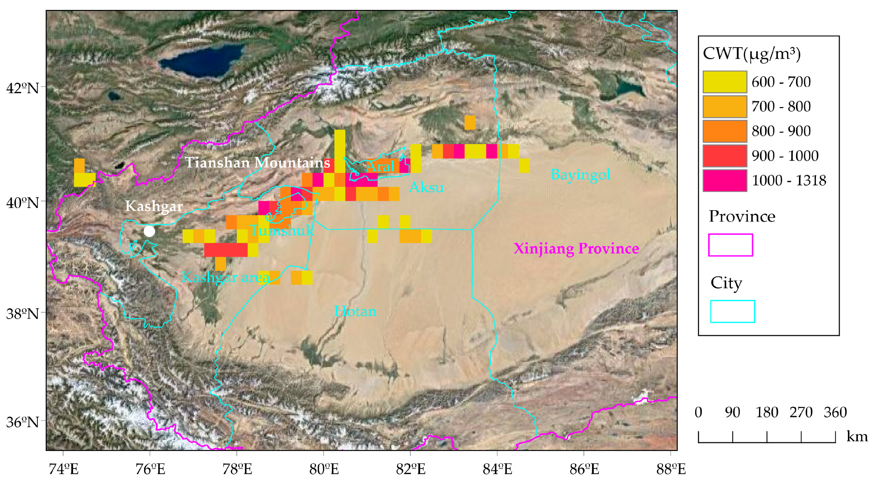
• This paper took Xi’an and Kashgar as examples to analyze joint governance regions based on pollution trajectories. In addition to local control, PM_2.5 control strategies during winter in Xi’an should include joint control with Nanchong, Guangan, Bazhong, and Dazhou in eastern Sichuan. PM_2.5 control in winter in Xi’an should also be coordinated with Ankang, Hanzhong, and Shangluo in southern Shaanxi to alleviate the problem of pollution sources in the south. Meanwhile, Xi’an should work with Weinan, Yanan, and Yuncheng to solve the problem of pollution sources in the northwest. For Kashgar, it is necessary to establish a PM_2.5 joint governance area along the Tianshan Mountains to the east, with a focus on joint governance with the northern cities of Kashgararea, Tumshuk, Aksuarea, and Aral in the east.

The method proposed in this paper can be used to analyze the joint governance regions and periods of PM_2.5 pollution in key cities across the entire country, and it can also be used in smaller areas, such as provinces or cities. The method is simple, feasible, and has universality. However, due to the many factors affecting the concentration of PM_2.5 and the limited space of this paper, the important influencing factors of PM_2.5 pollution prevention and control were not analyzed, which should be the focus of further research.

References

- Li, J.; Zhu, Y.; Kelly, J.T.; Jang, C.J.; Wang, S.; Hanna, A.; Xing, J.; Lin, C.-J.; Long, S.; Yu, L. Health benefit assessment of PM2.5 reduction in Pearl River Delta region of China using a model-monitor data fusion approach. J. Environ. Manage. 2019, 233, 489–498. [Google Scholar] [CrossRef] [PubMed]
- Zhao, P.; Zhang, X.; Xu, X.; Zhao, X. Long-term visibility trends and characteristics in the region of Beijing, Tianjin, and Hebei, China. Atmos. Res. 2011, 101, 711–718. [Google Scholar] [CrossRef]
- Wang, H.-J.; Chen, H.-P. Understanding the recent trend of haze pollution in eastern China: Roles of climate change. Atmos. Chem. Phys. 2016, 16, 4205–4211. [Google Scholar] [CrossRef] [Green Version]
- Xie, Y.; Dai, H.; Zhang, Y.; Wu, Y.; Hanaoka, T.; Masui, T. Comparison of health and economic impacts of PM2.5 and ozone pollution in China. Environ. Int. 2019, 130, 104881. [Google Scholar] [CrossRef] [PubMed]
- Wang, Y.; Yao, L.; Wang, L.; Liu, Z.; Ji, D.; Tang, G.; Zhang, J.; Sun, Y.; Hu, B.; Xin, J. Mechanism for the formation of the January 2013 heavy haze pollution episode over central and eastern China. Sci. China Earth Sci. 2014, 57, 14–25. [Google Scholar] [CrossRef]
- The Chinese State Council Atmosphere Pollution Prevention and Control Action Plan. Available online: http://www.gov.cn/zwgk/2013-09/12/content_2486773.htm (accessed on 2 February 2020).
- Li, D.; Zhao, Y.; Wu, R.; Dong, J. Spatiotemporal Features and Socioeconomic Drivers of PM2.5 Concentrations in China. Sustainability 2019, 11, 1201. [Google Scholar] [CrossRef] [Green Version]
- Chen, X.; Li, F.; Zhang, J.; Zhou, W.; Wang, X.; Fu, H. Spatiotemporal mapping and multiple driving forces identifying of PM2.5 variation and its joint management strategies across China. J. Clean. Prod. 2020, 250, 119534. [Google Scholar] [CrossRef]
- Jin, Q.; Fang, X.; Wen, B.; Shan, A. Spatio-temporal variations of PM2.5 emission in China from 2005 to 2014. Chemosphere 2017, 183, 429–436. [Google Scholar] [CrossRef]
- Wang, J.; Zhang, M.; Bai, X.; Tan, H.; Li, S.; Liu, J.; Zhang, R.; Wolters, M.A.; Qin, X.; Zhang, M. Large-scale transport of PM2.5 in the lower troposphere during winter cold surges in China. Sci. Rep. 2017, 7, 13238. [Google Scholar] [CrossRef] [Green Version]
- Wu, X.; Ding, Y.; Zhou, S.; Tan, Y. Temporal characteristic and source analysis of PM2.5 in the most polluted city agglomeration of China. Atmos. Pollut. Res. 2018, 9, 1221–1230. [Google Scholar] [CrossRef]
- Fang, C. Important progress and future direction of studies on China’s urban agglomerations. J. Geogr. Sci. 2015, 25, 1003–1024. [Google Scholar] [CrossRef] [Green Version]
- Chen, J.; Zhou, C.; Wang, S.; Hu, J. Identifying the socioeconomic determinants of population exposure to particulate matter (PM2.5) in China using geographically weighted regression modeling. Environ. Pollut. 2018, 241, 494–503. [Google Scholar] [CrossRef] [PubMed]
- Wang, J.; Wang, S.; Li, S. Examining the spatially varying effects of factors on PM2.5 concentrations in Chinese cities using geographically weighted regression modeling. Environ. Pollut. 2019, 248, 792–803. [Google Scholar] [CrossRef] [PubMed]
- Zhang, N.-N.; Ma, F.; Qin, C.-B.; Li, Y.-F. Spatiotemporal trends in PM2.5 levels from 2013 to 2017 and regional demarcations for joint prevention and control of atmospheric pollution in China. Chemosphere 2018, 210, 1176–1184. [Google Scholar] [CrossRef] [PubMed]
- Zhao, H.; Wang, T.; Jiang, F.; Xie, M. Investigation into the source of air pollutants to hong kong by using backward trajectory method during the trace-p campaign. J. Trop. Meteorol. 2009, 25, 181–186. [Google Scholar]
- Liao, T.; Wang, S.; Ai, J.; Gui, K.; Duan, B.; Zhao, Q.; Zhang, X.; Jiang, W.; Sun, Y. Heavy pollution episodes, transport pathways and potential sources of PM2.5 during the winter of 2013 in Chengdu (China). Sci. Total Environ. 2017, 584–585, 1056–1065. [Google Scholar] [CrossRef]
- Zhang, Z.Y.; Wong, M.S.; Lee, K.H. Estimation of potential source regions of PM2.5 in Beijing using backward trajectories. Atmos. Pollut. Res. 2015, 6, 173–177. [Google Scholar] [CrossRef] [Green Version]
- Kong, L.; Tan, Q.; Feng, M.; Qu, Y.; An, J.; Liu, X.; Cheng, N.; Deng, Y.; Zhai, R.; Wang, Z. Investigating the characteristics and source analyses of PM2.5 seasonal variations in Chengdu, Southwest China. Chemosphere 2020, 243, 125267. [Google Scholar] [CrossRef]
- Zeng, Y.; Cao, Y.; Qiao, X.; Seyler, B.C.; Tang, Y. Air pollution reduction in China: Recent success but great challenge for the future. Sci. Total Environ. 2019, 663, 329–337. [Google Scholar] [CrossRef]
- Mi, K.; Zhuang, R.; Zhang, Z.; Gao, J.; Pei, Q. Spatiotemporal characteristics of PM2.5 and its associated gas pollutants, a case in China. Sustain. Cities Soc. 2019, 45, 287–295. [Google Scholar] [CrossRef]
- Zhou, X.-L.; Wang, Q.; Shang, J.-G.; Liu, C.-S. Time Series Analysis for Pm2.5 and Pm10 in Beijing Based on Wavelet Transform Method; Khatib, J.M., Ed.; World Scientific Publ Co Pte Ltd.: Singapore, 2016; ISBN 978-981-4723-00-8. [Google Scholar]
- Fan, F.; Liu, R. Exploration of spatial and temporal characteristics of PM2.5 concentration in Guangzhou, China using wavelet analysis and modified land use regression model. Geo-spatial Inf. Sci. 2018, 21, 311–321. [Google Scholar] [CrossRef] [Green Version]
- Chen, X.; Yin, L.; Fan, Y.; Song, L.; Ji, T.; Liu, Y.; Tian, J.; Zheng, W. Temporal evolution characteristics of PM2.5 concentration based on continuous wavelet transform. Sci. Total Environ. 2020, 699, 134244. [Google Scholar] [CrossRef] [PubMed]
- Huang, P.; Zhang, J.; Tang, Y.; Liu, L. Spatial and Temporal Distribution of PM2.5 Pollution in Xi’an City, China. Int. Environ. Res. Public Health 2015, 12, 6608–6625. [Google Scholar] [CrossRef] [PubMed] [Green Version]
- Liang, Y.; Fang, L.; Pan, H.; Zhang, K.; Kan, H.; Brook, J.R.; Sun, Q. PM2.5 in Beijing - temporal pattern and its association with influenza. Environ. Health 2014, 13, 102. [Google Scholar] [CrossRef] [Green Version]
- Feng, X.; Li, Q.; Zhu, Y.; Hou, J.; Jin, L.; Wang, J. Artificial neural networks forecasting of PM2.5 pollution using air mass trajectory based geographic model and wavelet transformation. Atmos. Environ. 2015, 107, 118–128. [Google Scholar] [CrossRef]
- Mahajan, S.; Liu, H.-M.; Tsai, T.-C.; Chen, L.-J. Improving the Accuracy and Efficiency of PM2.5 Forecast Service Using Cluster-Based Hybrid Neural Network Model. IEEE Access 2018, 6, 19193–19204. [Google Scholar] [CrossRef]
- Prakash, A.; Kumar, U.; Kumar, K.; Jain, V.K. A Wavelet-based Neural Network Model to Predict Ambient Air Pollutants’ Concentration. Environ. Model. Assess. 2011, 16, 503–517. [Google Scholar] [CrossRef]
- Gan, C.-M.; Wu, Y.; Madhavan, B.L.; Gross, B.; Moshary, F. Application of active optical sensors to probe the vertical structure of the urban boundary layer and assess anomalies in air quality model PM2.5 forecasts. Atmos. Environ. 2011, 45, 6613–6621. [Google Scholar] [CrossRef]
- Zhang, H.; Zhang, S.; Wang, P.; Qin, Y.; Wang, H. Forecasting of particulate matter time series using wavelet analysis and wavelet-ARMA/ARIMA model in Taiyuan, China. J. Air Waste Manage. Assoc. 2017, 67, 776–788. [Google Scholar] [CrossRef] [Green Version]
- Mao, T.; Wan, W.; Yue, X.; Sun, L.; Zhao, B.; Guo, J. An empirical orthogonal function model of total electron content over China. Radio Sci. 2008, 43, 1–12. [Google Scholar] [CrossRef]
- Duan, X.; Gu, Z.; Li, Y.; Xu, H. The spatiotemporal patterns of rainfall erosivity in Yunnan Province, southwest China: An analysis of empirical orthogonal functions. Global Planetary Chang. 2016, 144, 82–93. [Google Scholar] [CrossRef]
- Li, Q.; Chen, P.; Sun, L.; Ma, X. A global weighted mean temperature model based on empirical orthogonal function analysis. Adv. Space Res. 2018, 61, 1398–1411. [Google Scholar] [CrossRef]
- Li, L.; Gottschalk, L.; Krasovskaia, I.; Xiong, L. Conditioned empirical orthogonal functions for interpolation of runoff time series along rivers: Application to reconstruction of missing monthly records. J. Hydrol. 2018, 556, 262–278. [Google Scholar] [CrossRef]
- Kim, S.E.; Seo, I.W.; Choi, S.Y. Assessment of water quality variation of a monitoring network using exploratory factor analysis and empirical orthogonal function. Environ. Modelling Soft. 2017, 94, 21–35. [Google Scholar]
- Chen, P.; Liu, L.; Yao, Y.; Yao, W. A global empirical orthogonal function model of plasmaspheric electron content. Adv. Space Res. 2020, 65, 138–151. [Google Scholar] [CrossRef]
- Xu, G.; Ren, X.; Xiong, K.; Li, L.; Bi, X.; Wu, Q. Analysis of the driving factors of PM2.5 concentration in the air: A case study of the Yangtze River Delta, China. Ecological Indicators 2020, 110, 105889. [Google Scholar] [CrossRef]
- Lai, S.; Zou, S.; Cao, J.; Lee, S.; Ho, K. Characterizing ionic species in PM2.5 and PM10 in four Pearl River Delta cities, South China. J. Environ. Sci. 2007, 19, 939–947. [Google Scholar] [CrossRef]
- Gao, H.; Yang, W.; Yang, Y.; Yuan, G. Analysis of the Air Quality and the Effect of Governance Policies in China’s Pearl River Delta, 2015–2018. Atmosphere 2019, 10, 412. [Google Scholar] [CrossRef] [Green Version]
- Yan, D.; Lei, Y.; Shi, Y.; Zhu, Q.; Li, L.; Zhang, Z. Evolution of the spatiotemporal pattern of PM2.5 concentrations in China – A case study from the Beijing-Tianjin-Hebei region. Atmos. Environ. 2018, 183, 225–233. [Google Scholar] [CrossRef]
- PM25. Available online: http://www.pm25.in/ (accessed on 2 February 2020).
- National Urban Air Quality Real-Time Release Platform. Available online: http://106.37.208.233:20035/ (accessed on 2 February 2020).
- Hsu, Y.-M.; Wang, X.; Chow, J.C.; Watson, J.G.; Percy, K.E. Collocated comparisons of continuous and filter-based PM2.5 measurements at Fort McMurray, Alberta, Canada. J. Air Waste Manag. Associ. 2016, 66, 329–339. [Google Scholar]
- How Inverse Distance Weighted Interpolation Works. Available online: https://pro.arcgis.com/en/pro-app/help/analysis/geostatistical-analyst/how-inverse-distance-weighted-interpolation-works.htm (accessed on 18 February 2020).
- Su, L.; Yuan, Z.; Fung, J.C.H.; Lau, A.K.H. A comparison of HYSPLIT backward trajectories generated from two GDAS datasets. Sci. Total Environ. 2015, 506–507, 527–537. [Google Scholar] [CrossRef] [PubMed]
- North, G.; Bell, T.; Cahalan, R.; Moeng, F. Sampling Errors in the Estimation of Empirical Orthogonal Functions. Monthly Weather Rev. 1982, 110, 699–706. [Google Scholar] [CrossRef]
- Grinsted, A.; Moore, J.; Jevrejeva, S. Application of Cross Wavelet Transform and Wavelet Coherence to Geophysical Time Series. Nonlinear Processes Geophys. 2004, 11, 561–566. [Google Scholar] [CrossRef]
- Torrence, C.; Compo, G.P. A Practical Guide to Wavelet Analysis. Bulletin Am. Meteorol. Soc. 1998, 79, 61–78. [Google Scholar] [CrossRef] [Green Version]
- Teolis, A. Computational Signal Processing with Wavelets; Birkhäuser: Boston, NY, USA, 1985. [Google Scholar]
- He, P.; Li, P.; Sun, H. Feature Extraction of Acoustic Signals Based on Complex Morlet Wavelet. Procedia Eng. 2011, 15, 464–468. [Google Scholar] [CrossRef] [Green Version]
- Draxler, R.R. The Use of Global and Mesoscale Meteorological Model Data to Predict the Transport and Dispersion of Tracer Plumes over Washington, D.C. Wea. Forecasting 2006, 21, 383–394. [Google Scholar] [CrossRef]
- Stein, A.F.; Draxler, R.R.; Rolph, G.D.; Stunder, B.J.B.; Cohen, M.D.; Ngan, F. NOAA’s HYSPLIT Atmospheric Transport and Dispersion Modeling System. Bull. Amer. Meteor. Soc. 2015, 96, 2059–2077. [Google Scholar] [CrossRef]
- Song, Z.; Bai, X. An Overview of RSMC Beijing Modeling System for Trajectories, Dispersion and Deposition; IEEE International Symposium on Geoscience and Remote Sensing: Denver, CO, USA, 2006; pp. 3361–3364. [Google Scholar]
- Draxler, R.R.; Gillette, D.A.; Kirkpatrick, J.S.; Heller, J. Estimating PM10 air concentrations from dust storms in Iraq, Kuwait and Saudi Arabia. Atmos. Environ. 2001, 35, 4315–4330. [Google Scholar] [CrossRef]
- Wang, J.; Wang, S.; Jiang, J.; Ding, A.; Zheng, M.; Zhao, B.; Wong, D.C.; Zhou, W.; Zheng, G.; Wang, L.; et al. Impact of aerosol–meteorology interactions on fine particle pollution during China’s severe haze episode in January 2013. Environ. Res. Lett. 2014, 9, 094002. [Google Scholar] [CrossRef]
- Wang, Y.Q.; Zhang, X.Y.; Draxler, R.R. TrajStat: GIS-based software that uses various trajectory statistical analysis methods to identify potential sources from long-term air pollution measurement data. Environ. Modelling Softw. 2009, 24, 938–939. [Google Scholar]
- Hsu, Y.-K.; Holsen, T.M.; Hopke, P.K. Comparison of hybrid receptor models to locate PCB sources in Chicago. Atmos. Environ. 2003, 37, 545–562. [Google Scholar] [CrossRef]
- Han, Y.-J.; Holsen, T.M.; Hopke, P.K.; Yi, S.-M. Comparison between Back-Trajectory Based Modeling and Lagrangian Backward Dispersion Modeling for Locating Sources of Reactive Gaseous Mercury. Environ. Sci. Technol. 2005, 39, 1715–1723. [Google Scholar] [CrossRef] [PubMed]
- Wang, Y.Q.; Zhang, X.Y.; Arimoto, R. The contribution from distant dust sources to the atmospheric particulate matter loadings at XiAn, China during spring. Sci. Total Environ. 2006, 368, 875–883. [Google Scholar] [CrossRef] [PubMed]
- Petre, S.; Randolph, L.M. Spectral Analysis of Signals; Prentice Hall: Upper Saddle River, NJ, USA, 2005. [Google Scholar]
- MathWorks China Find Periodicity Using Autocorrelation. Available online: https://ww2.mathworks.cn/help/signal/ug/find-periodicity-using-autocorrelation.html?lang=en (accessed on 20 February 2020).