Article

Impacts of Climate Change and Different Crop Rotation Scenarios on Groundwater Nitrate Concentrations in a Sandy Aquifer

1
School of Engineering, University of Guelph, Guelph, ON N1G 2W1, Canada
2
Plant Agriculture, University of Guelph, Guelph, ON N1G 2W1, Canada
*
Author to whom correspondence should be addressed.
Sustainability 2020, 12(3), 1153; https://doi.org/10.3390/su12031153
Submission received: 4 January 2020 / Revised: 29 January 2020 / Accepted: 2 February 2020 / Published: 5 February 2020
(This article belongs to the Special Issue Watershed Processes under Changing Climate)

Abstract

:
Nitrate in groundwater is a major concern in agricultural sub-watersheds. This study assessed the impacts of future climate and agricultural land use changes on groundwater nitrate concentrations in an agricultural sub-watershed (Norfolk site) in southern Ontario, Canada. A fully integrated hydrologic model (HydroGeoSphere) was used in combination with the root zone water quality model (RZWQM2) (shallow zone) to develop water flow and nitrate transport models. Three climate change models and three crop rotations (corn-soybean rotation, continuous corn, corn-soybean-winter wheat-red clover rotation) were used to evaluate the potential impact on groundwater quality (nine predictive scenarios). The selected climate change scenarios yielded less water availability in the future period than in the reference period (past conditions). The simulated nitrate nitrogen (Nitrate-N) concentrations were lower during the future period than the reference period. The continuous corn land use scenario produced higher Nitrate-N concentrations compared to the base case (corn-soybean rotation). However, the best management practices (BMP) scenario (corn-soybean-winter wheat-red clover rotation) produced significantly lower groundwater nitrate concentrations. BMPs, such as the one examined herein, should be adopted to reduce potential negative impacts of future climate change on groundwater quality, especially in vulnerable settings. These findings are important for water and land managers, to mitigate future impacts of nutrient transport on groundwater quality under a changing climate.

1. Introduction

Climate has always played an important role in the agriculture industry and has shaped the outlook of agriculture all over the world [1,2]. Farmers select their crops based on climatic factors such as annual rainfall, low and high temperatures, and growing season length [3,4]. In recent decades, farming activities in agricultural watersheds have become a major concern for water quantity and quality [5,6]. Conventional farming practices in some locations were to apply fertilizers uniformly at high rates without considering the crop and soil requirements [7,8,9] resulting in leaching of excess nutrients to groundwater especially after a heavy rainfall event [9]. However, more farmers are moving towards better nutrient management considering the negative impacts of high fertilizer rates on crop productivity and the environment [10,11,12]. Elevated concentrations of nitrogen and phosphorous in water bodies can cause many health and environmental problems, such as methemoglobinemia (blue baby syndrome) and eutrophication, respectively [13,14]. Therefore, it is necessary to evaluate the impact of land and crop management practices on groundwater quality under changing climate conditions.
Anthropogenic activities have also affected water quantity for both surface and groundwater resources, although groundwater is considered to be less impacted in terms of quality, due to filtration of the water through different geological materials in the subsurface [15]. About 30% of the Canadian population depends on groundwater as the main or only source of drinking water [16]. In Ontario, about 28% of the population is reliant on groundwater while many rural communities entirely rely on groundwater for both drinking and irrigation purposes [16]. Groundwater may be used to irrigate crops, especially during periods of drought to meet crop water requirements. Continuous pumping of groundwater can increase the risks of groundwater depletion which can not only compromise the future groundwater supply [17] but also can reduce river baseflow and affect aquatic life [18,19]. Therefore, it is very important to protect the quality and quantity of groundwater stored in aquifers to ensure safe water supply for future generations [20].
In addition to field-based studies, numerical models are useful tools to provide insights into water flow and nutrient transport dynamics from agricultural fields to hydrological receptors [21,22,23,24,25,26,27,28]. Numerical models for subsurface water modeling have further been categorized as vadose zone and saturated zone models. RZWQM2 (root zone water quality model) [26], DRAINMOD-NII [24], leaching estimation and chemistry model (LEACHM) [29], and HYDRUS [23] are the main vadose zone one-dimensional (1D) models currently in use to simulate flow and transport through the root zone from different cropping systems. MODFLOW [22], MIKE SHE [30], FEFLOW [28], HydroGeoSphere (HGS) [25], and various other numerical models can simulate three-dimensional (3D) flow and contaminant transport through groundwater, while MIKE SHE and HGS are examples of fully integrated models that can simulate both surface and groundwater flow and transport [31,32,33]. Realistic conceptualization of the study areas along with proper calibration and validation of these numerical models can not only provide a platform to examine the complex hydrological processes but it can also help to evaluate the impacts of future land use and climate changes.
Climate change modeling is a challenging and difficult task since there are many uncertainties involved and climate science is an evolving subject. General circulation models (GCMs) have been developed to provide global-scale climate projections and have been widely used worldwide. The GCMs can be further downscaled at a finer resolution to obtain more realistic local-scale climate projections by using statistical or dynamical downscaling techniques [34]. Regional climate models (RCMs) are available for many regions across Canada [34]. Extracted future climate data can be inputted into groundwater modeling tools to examine the impact of climate changes on groundwater quantity and quality.
Most of the previous studies conducted to examine the impacts of climate change on groundwater in Canada were focused on water quantity rather than quality [18,27,35,36,37,38,39,40,41,42,43,44]. Very little research has been done on a subwatershed scale to develop fully integrated models with different crop rotations to simulate both water flow and agricultural nitrate transport in groundwater considering future climate change [27,37,45,46,47]. The primary objective of this study is examine the impacts of climate change (for the 2040-2059 period) and land use changes (focused on three crop rotation scenarios) on Nitrate-N concentrations in groundwater using integrated numerical modeling tools. Secondly, this study aims to compare the impact of different climate change scenarios and crop rotation scenarios on groundwater elevation and surface water flow at the outlet of the examined watershed. It is anticipated that this modeling approach will provide useful insights for the selection of best management practices (BMPs) to minimize the impacts of agricultural activities on water quality and quantity. Furthermore, similar studies can be conducted in various hydrogeological settings and cropping systems to develop a comprehensive plan to delineate vulnerable areas to groundwater nitrate contamination especially considering the future climate changes in agricultural watersheds.

2. Materials and Methods
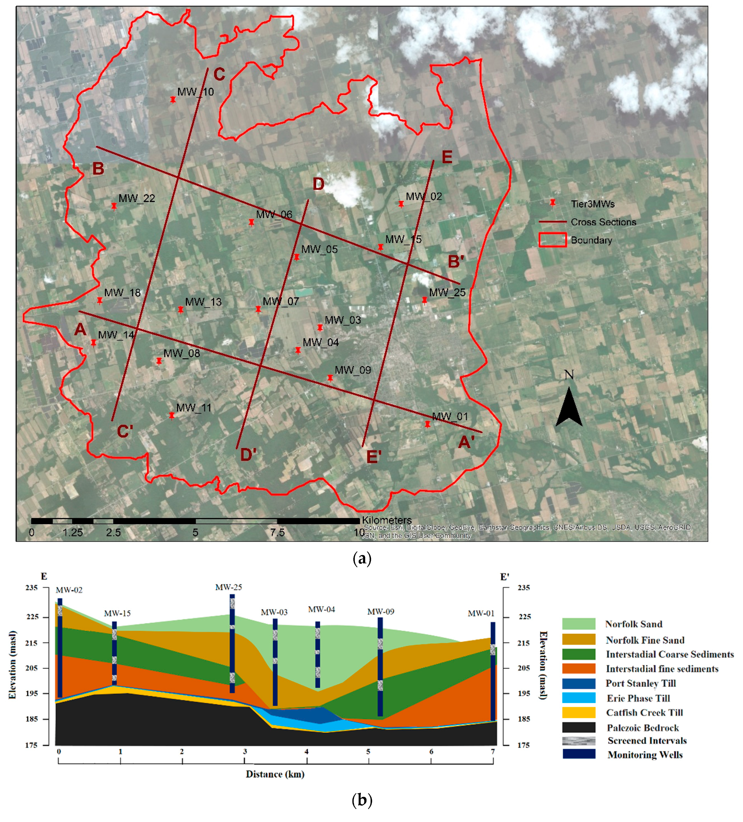
2.1. Study Site

The Norfolk research site with a catchment area of 155 km2 (Figure 1) is located in Norfolk County in southwestern Ontario and it is part of the Lynn River sub-watershed. The average annual precipitation at for the 2010–2016 period was 1009 mm (ranging between 830 to 1349 mm) [48]. Both surface water and groundwater flows from northwest to southeast in this sub-watershed. The river outlet is located at the southeastern boundary of the modelled domain and the surface elevation varies from 188 to 265 meters above sea level (masl). The study site is dominated by cultivated crops (mainly corn (~16%–25%), soybeans (~16%–25%), and specialty crops (~15%)) except near the southwestern boundary, where forest covers large areas of the research site [49].

2.2. Hydrogeological Modeling

2.2.1. Geological and Hydrogeological Framework

The study site is comprised of the Norfolk sand plain, having a thick layer of unconsolidated material above the Paleozoic bedrock. Borehole data from monitoring wells installed for a Tier 3 (water budget and local risk assessment) source water protection study [51] was used to create a conceptual model for the study site with detailed definition of geological and hydrogeological layers (Figure 2).
The top layer, commonly known as Norfolk sand plain (Whittlesey/Warren phase), identified as a thick layer of sand laid during the end of the Huron stadial consists of the most recent lake sediments. Whittlesey/Warren phase sediments are made up of medium sand or fine sand to medium sand and is split into two sublayers based on material grading [52]. The sublayer comprised of fine sand sediments sits at the bottom of the coarse-to-medium sand sublayer [52]. All shallow monitoring wells are screened in the Norfolk coarse sand layer and have high hydraulic conductivity (K) ranging from 5.5 × 10⁻⁴ m s−1 to 3.6 × 10⁻⁴ m s−1 [51]. The Norfolk fine sand layer has relatively lower K that ranges from 4.2 × 10⁻⁵ m s−1 to 3.6 ×10⁻⁷ m s−1 [51].
The Norfolk fine sand layer is underlain by an Interstadial coarse sand layer (Ypsilanti layer) that represents a well-defined period of quick drops in lake levels resulting in relatively coarser sediments [52]. The Interstadial coarse sediment layer also has high K and deep wells are mostly screened in this layer with K ranging from 5.6 × 10⁻⁶ to 1.70 × 10⁻³ m s−1 [51]. The Interstadial fine sediment layer (Lake Maumee/Arkona) is dominated by a low energy deposition of very fine to fine sediments (very fine sand to clay) [52]. The thickness of the Interstadial fine sediment layer increases towards the east within the study area and it is present throughout all cross-sections.
The Port Stanley Till layer represents re-advance of the Erie lobe during the Port Burce stadial picked up the older Erie phase glaciolacustrine deposits and consists a clayey silt to sandy silt diamicton with a small percentage of coarse sediments [52]. The Erie Phase layer consists of glaciolacustrine sediments comprised of bedded sand, and silt and clay layers represent a period of ice retreat referred to as the Erie interstadial [53]. The Catfish Creek Till layer is the smallest and oldest sediment layer delineated that comprises a gravelly sandy till which correlates to the Nissouri stadial [52]. The Paleozoic bedrock is very deep (> 30 m below ground surface) and acts as an aquitard [54].
Tritium and other stable isotopes analyses on groundwater samples collected during field work in July 2014 indicated that modern groundwater is present at the research site [55]. The isotope results showed that the recharge water is only 5 to 10 years old at the research site and the position of the data relative to the global meteoric water line indicates cold climate region groundwater [55,56]. The nitrogen-15 isotope results indicated that agricultural activities are the main source of groundwater Nitrate-N concentrations at the research site, with only one well location where a septic system was identified as the main cause of groundwater Nitrate-N concentrations [55]. High infiltration rates and the sandy nature of the soil indicates that most of the contribution from the subwatershed to the Lynn river is through baseflow. The regional groundwater flows from northwest to southeast towards the Lake Erie.
In summary, the developed conceptual hydrogeological model indicates that the groundwater flow and Nitrate-N transport occur in unconsolidated shallow sand layers with high K. The groundwater present at the research site is relatively fresh and nitrate transported to the aquifer by infiltration will first reach the shallow groundwater and will flow southwards towards Lake Erie. The water quality in the aquifer can be controlled by water infiltration (recharge) and nitrate leaching from the catchment area
Cross-sections were made using all Tier-3 monitoring wells and elevation points were inferred from these geologic cross sections. The geological layers were interpolated at a resolution of 1 × 1 m using an inverse distance weighted scheme and the bottom of the conceptual model was set at the top of bedrock (175 masl). A total of nine hydrogeological layers were selected for numerical modeling purposes (Figure 2).

2.2.2. Numerical Modeling

A two-step numerical modeling approach was adopted for this study. A 1D vadose zone crop model RZWQM [26], was selected to model the detailed crop growth and Nitrate-N leaching though the root zone. The RZWQM2 model was calibrated and validated for various cropping systems using soil and leachate data from soil samples and suction lysimeters installed in the selected fields. The RZWQM2 model outputs such as daily Nitrate-N mass and daily leaf area index (LAI) were used as inputs in the integrated hydrological model. The field-scale RZWQM2 model provides comprehensive outputs in terms of plant growth and vadose zone hydrogeology that can be neglected in watershed scale models. The detailed vadose zone modeling procedure is described in Reference [57].
A fully integrated (surface-subsurface) HGS model was used to simulate groundwater flow and transport of Nitrate-N in the groundwater at the study site. HGS uses a two-dimensional (2D) wave approximation of the Saint Venant equation [58] for surface flow. The finite-element approach was selected for groundwater modeling and Algomesh [59] was used to create a 2D mesh of the study site. The Saint Venant equation to quantify surface flow requires Manning coefficients that are used to calculate friction slopes, and a specified rill storage height to determine how much water is stored in the surface depressions. Rill storage is an important factor in rural settings and influences the surface runoff generated from the study site. Another important parameter for the surface flow simulation is the coupling length between the surface and subsurface domains [60]. All the overland flow properties were assumed to be uniform throughout the study area. The model uses the Richards’ equation [61] to calculate three-dimensional (3D) subsurface flow in variably saturated media. Evapotranspiration (ET) affecting both the surface and subsurface domains is modelled as a combination of plant transpiration and evaporation following the approach described in Reference [62]. The rate of transpiration from the modeling domain depends on LAI, root distribution function, and variability in available soil moisture content. Transpiration nonlinearly depends on soil moisture content and wilting point (θwp), field capacity (θfc), oxic limit (θo), and anoxic limit (θan). Maximum rooting depths and root extraction functions are also important factors in simulating evapotranspiration.

2.2.3. Data Collection

A hydrologically enforced digital elevation model (DEM) was provided by the Grand River Conservation Authority (GRCA) with a resolution of 1 × 1 m. Land use data for the study site was downloaded from the Agriculture and Agri-food Canada (AAFC) website [49]. At the site, groundwater elevation and Nitrate-N data was collected from selected monitoring wells on a bi-monthly basis, from June 2014 to July 2016 [55]. Outflow data was collected for 1990-2016 from a Water Survey of Canada gauge near the outlet of the watershed [63]. The climate data, including precipitation and temperature, were collected from the local weather station [48]. The solar radiation data for both sites was downloaded from NASA at a spatial resolution of 0.5° × 0.5° [64]. Potential evapotranspiration (PET) zones were delineated based on different land uses. Details of data types, spatial and temporal resolutions, and data sources are described in Table 1.

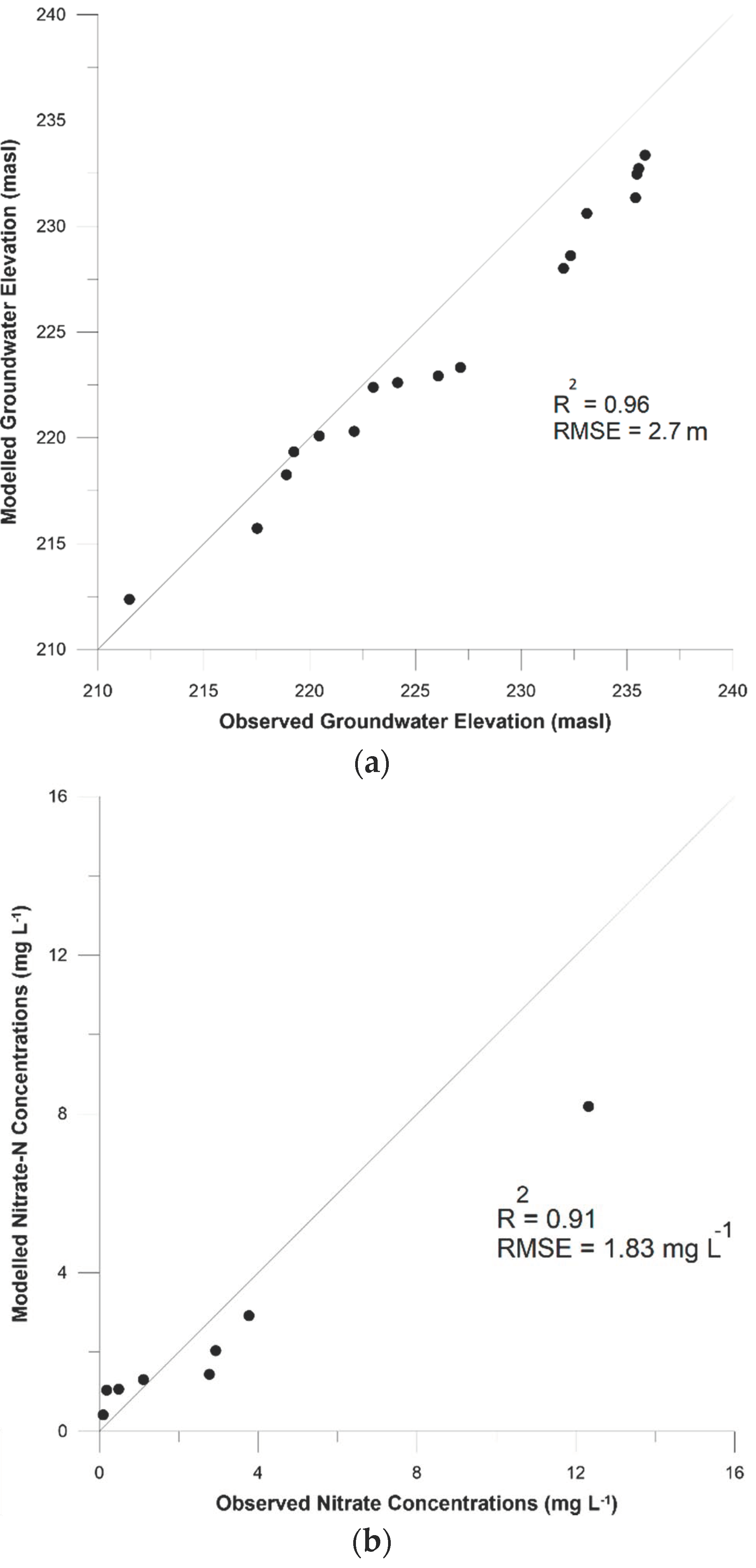
2.2.4. Model Calibration and Validation.

The 3D HGS model for the study site consists of 222,363 nodes and 415,560 elements. A critical depth boundary condition was applied in HGS at the watershed outlet with all other boundaries specified as no flow. The horizontal and vertical hydraulic conductivities (Kxy and Kz, respectively) along with surface flow and evapotranspiration parameters for various cropping systems were calibrated during the “steady state” calibration. Some of the parameter values were adopted from the literature values.
For initial conditions, a spin up period (1000 years) was used to obtain reasonable groundwater elevation and flow values and avoid inappropriate initial conditions. The initial conditions were based on average rainfall and PET (1990–2009) and average values for Nitrate-N concentrations from different land use types generated in RZWQM2. Once the initial heads and concentrations were obtained, the model was calibrated for steady state conditions. The PEST software package [65] was used to calibrate the K values and average outlet flow for the study area. Transpiration and evaporation limiting saturations and canopy storage parameters were also calibrated to match the evapotranspiration generated by RZWQM2. Results showed a good agreement between modelled and observed groundwater elevations (masl) with an R2 value of 0.96 and a root mean square error (RMSE) of 2.7 m (Figure 3a). Similarly, observed and modelled Nitrate-N concentrations in sampled monitoring wells also had a good agreement with an R2 value of 0.91 and a RMSE of 1.83 mg L−1 (Figure 3b). The final calibrated values of all input parameters are provided in Table 2, Table 3, and Table 4.
The steady state calibration was followed by transient state calibration and validation with a special focus to adjust the transport parameters, such as dispersivities and the specific storage to accurately model the Nitrate-N in the groundwater. The outflow was calibrated for 2013–2014 and validated for 2015–2016, while the groundwater elevation and groundwater Nitrate-N concentrations were spatially calibrated and validated. Automatic calibration software PEST-HP [65] was used for transient state parameters [57]. The detailed transient state calibration and validation results can be accessed in Reference [57]. For this reason, only a brief description of the data calibration and validation procedure is included in this paper. Calibrated values of the transient state parameters are provided in Table 5. The calibrated model was used for the evaluation of crop rotation scenarios and climate change projections in this study.

2.2.5. Sensitivity Analysis

Relative Sensitivity (Sr) of averaged groundwater elevation, outflow, and groundwater Nitrate-N concentrations was evaluated using a procedure adopted from Reference [75] under steady state conditions. The calibration parameters subjected to sensitivity analysis were K, precipitation, and PET (Table 6). The K values selected for sensitivity analysis were based on maximum and minimum field calculated for Layers 1–3 and Layers 4–5 (Table 2). For climate parameters, maximum and minimum values between 2010 to 2016 were selected [48]. The absolute value of Sr may vary from 0 to infinity with smaller values representing a more robust model (minor changes in output by changing the parameter values) while larger values represent greater parameter sensitivity.
Sensitivity analysis results showed that both outflow and groundwater Nitrate-N concentrations were more sensitive to the modified parameters than groundwater elevation. All three model outputs were more sensitive to the changes in precipitation and PET compared to changes in K. Only groundwater Nitrate-N was sensitive to changes in K values for Layers 1–3 (Table 6). These results indicate that climate change and crop coverage can highly influence the model outputs.

2.3. Future Climate Projections

Dynamically downscaled regional climate model (RegCM) climate change projections (25 km resolution) under the representative concentration pathway (RCP) 8.5 emission scenario and driven by five global climate models (GCMs) (CanESM2, HadGEM2-ES, GFDL-ESM2M, IPSL-CM5A-LA, and MPI-ESM-MR) were downloaded from the Ontario Climate Change Data Portal (CCDP) [76]. This data corresponds to a reference period spanning from 1986 to 2005 with focus on a mid-century future period (2040-2059). Regional dynamic downscaling provides better representation of extreme and mean climate conditions than statistical downscaling [77]. The selection of climate change projections was based on future temperature and precipitation changes relative to the reference period. The criteria were to select a projection with maximum precipitation change and temperature change, minimum precipitation change and maximum temperature change, and business as usual (both temperature and precipitation change close to observed data). To assess this, the annual means of climate change projections from all five driving GCMs for the reference period were compared (Figure 4). The MPI (MPI-ESM-MR) projection was selected for the highest precipitation changes, CanESM (CanESM2) was selected for the highest temperature and lowest precipitation change, and GFDL (GFDL-ESM2M) was initially selected as a business as usual scenario based on annual temperature and precipitation changes for the reference period.
However, monthly mean temperature (Figure 5a) and precipitation (Figure 5b) data showed that HadGEM (HadGEM2-ES) better represents the observed condition for the reference period and it was selected as a replacement for the GFDL scenario. The final three climate change scenarios used for this study were CanESM, HadGEM, and MPI. For the study site, local climate data was downloaded from Environment and Climate Change Canada for the reference period (1986-2005) [48]. The average observed annual and monthly precipitation for the reference period was 976.71 mm and 80.61 mm, respectively [48]. The observed temperature during the reference period ranged between −24 °C and 29 °C [48], while the climate models’ minimum and maximum temperatures for the reference period were: CanESM: −15.7 °C and 29 °C; HadGEM: −23.7 °C and 30.3 °C; and MPI: −24 °C and 29 °C. Several studies have suggested the application of a bias correction technique before using the RCM data in order to better represent the local subwatershed scale climatic conditions [78,79,80,81]. There are different methods to bias correct the climate data which include the delta change approach, local intensity scaling, daily bias correction, and quantile mapping [82]. For this study, a quantile mapping technique was used to remove the biases between simulated and observed temperature and precipitation variables. Details of the quantile mapping technique are described in [82]. The net recharge (Pnet), that is precipitation-PET, was calculated on a monthly basis to estimate the variation in water available for potential recharge and surface runoff throughout the year. PET was calculated using the Penman–Monteith equation [83]. Once the climate models were corrected for their bias, outputs for the average monthly temperature and precipitation for the reference period were reproduced.

2.4. Crop Rotation Scenarios

Many different agricultural land use change scenarios can be devised, including those based on crop area coverage, forestation/deforestation, urban/rural area coverage, etc. In the current study, the focus was to define and quantify the transport of excess nutrients, specifically nitrogen related to cash crop modifications and variable weather, into groundwater to anticipate and mitigate potential water quality impacts. Three future crop scenarios were selected to consider potential variation and extremes in nitrogen application: (1) crop area under corn-soybean rotation will continue to be under the same corn-soybean rotation in the future (business as usual scenario or base case scenario), (2) crop area under corn-soybean rotation changes to continuous corn plantation (cash crops only) in the future (worst case scenario), and (3) crop area under corn-soybean rotation changes to corn-soybean-winter wheat-red clover rotation (BMP scenario).

2.5. Statistical Evaluation

The surface flow at the watershed outlets as well as groundwater elevation and Nitrate-N concentrations in monitoring wells were compared based on four seasons: winter (Dec, Jan, Feb), spring (Mar, Apr, May), summer (June, July, Aug), and fall (Sep, Oct, Nov). This quarterly comparison provides useful insight on how future climate change will vary seasonally and how it will impact Nitrate-N concentrations during the growing season relative to the rest of the year. Box plots were created to compare the data distribution based on percentile for groundwater elevation, surface flow, and Nitrate-N concentrations for each season using Grapher 11 (Golden Software, LLC, Golden, CO, USA). The ensemble means of surface water, groundwater elevations, and nitrate concentrations were compared using one-way analysis of variance (ANOVA) followed by means comparison using a least significant difference (LSD) for significantly different treatments (p < 0.05) in SPSS (IBM SPSS®, New York, NJ, USA).

3. Results

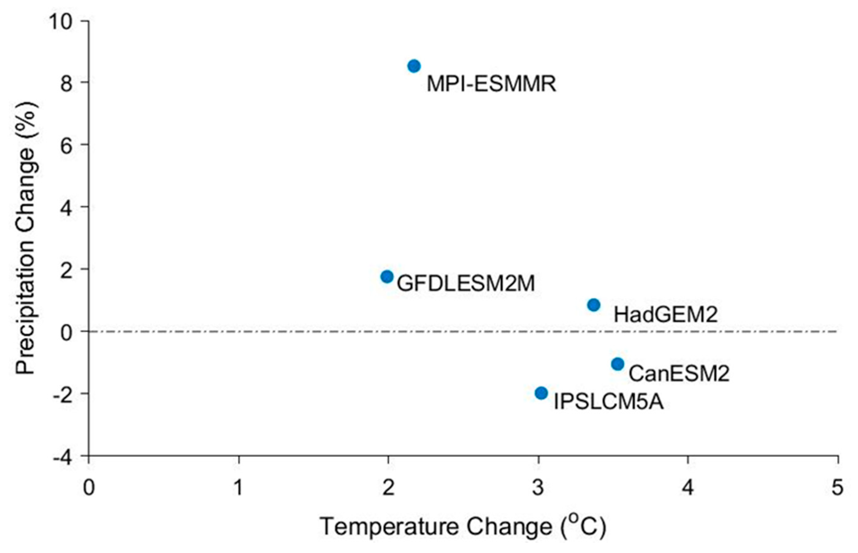
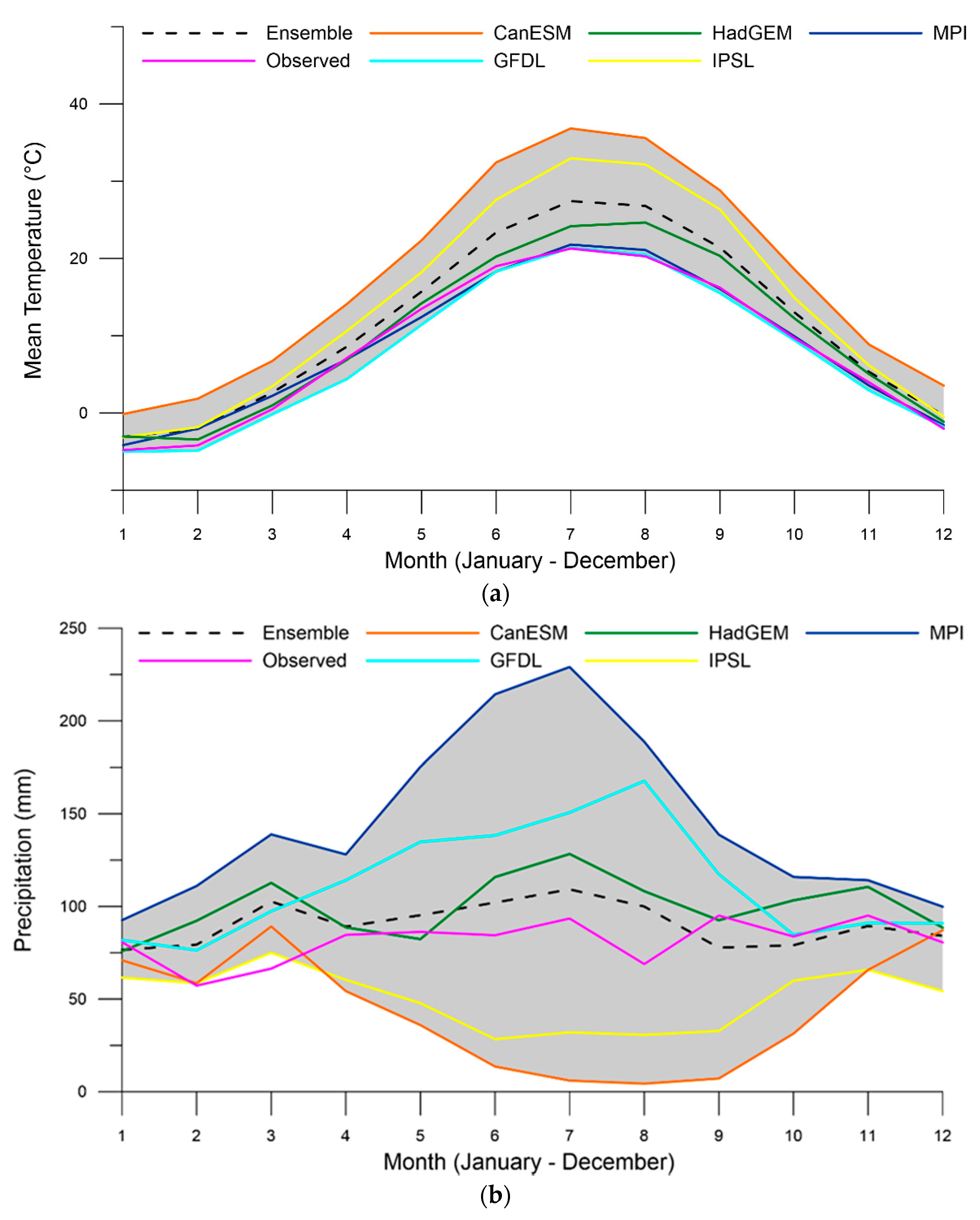
3.1. Climate Projections

The ensemble means of future (2040–2059) simulations predicted an increase of 0.37 °C (May) to 0.19 °C (February) for monthly temperatures (Figure 6a). The envelope of uncertainty remains relatively equal throughout the year except for March, in which the MPI scenario showed a decrease of 1.3 °C in mean temperature between future and historic model data. The ensemble means of future simulations predicted an increase in monthly precipitation for every month from December to April and a decrease in monthly precipitation from the months of May to November (Figure 6b). All three models suggest high precipitation during winter months. The CanESM model showed an erratic behavior for precipitation change between future and reference periods during the summer months. The envelope of uncertainty remains high (6% to 59%) and the ensemble means predicted less rainfall in the future during the growing season (May to October) (Figure 6b). The ensemble means of calculated Pnet values had a maximum increase of 27.4 mm in April and a maximum decrease of 19.8 mm in July. The envelope of uncertainty showed a range between 1 mm (April) and 45 mm (August). Pnet variations were high between different models during the months of July to September (Figure 6c). The envelope of uncertainty for temperature change also had similar trends for these months (Figure 6a). Overall, the envelope of uncertainty for Pnet illustrated that the growing season (May to October) has less available water for potential surface runoff and groundwater recharge; however, the actual rate of availability depends on which model represents the future climate conditions more accurately (Figure 6c).
Overall, the envelope of uncertainty indicated that future growing seasons will have less available water for potential surface runoff and groundwater recharge compared to the past. However, the rate of availability depends on which model will represent the future climate conditions more accurately at the study site (Figure 6c).

3.2. Numerical Modeling Results

The calibrated HGS model was run for three bias-corrected climate change scenarios and three land use change scenarios for both the reference (1986–2005) and future periods (2041–2059). The seasonal variation of (a) surface water flow at the outlet, (b) groundwater elevation at the monitoring wells, and (c) groundwater Nitrate-N concentrations at the monitoring wells were studied. Statistical analysis in terms of the ensemble averages was also studied for each monitoring well.

3.2.1. Outflow

Outflow at the study site was higher for the reference period compared to the future period for all three climate change scenarios and flow at the outlet ranged from 0.75 to 2.1 m3 s−1 (Figure 7). The monthly Pnet (Figure 6c) values at the study site indicated that the amount of water available for hydrologic processes throughout the winter and spring months was close to zero for the reference and future periods, while the amount of water available for hydrologic processes for summer and fall months were less for the future period compared to the reference period. Higher flows at the outlet were more prominent during summer and fall periods for the study site (Figure 7).
The average values for model ensemble outflows at the study site for the reference and future periods were 1.12 and 1.09 m3 s−1, respectively (Table 7). The results for the model ensemble indicated that the outflow will be decreased (statically significant) in the future period by 2.86% at the study site.

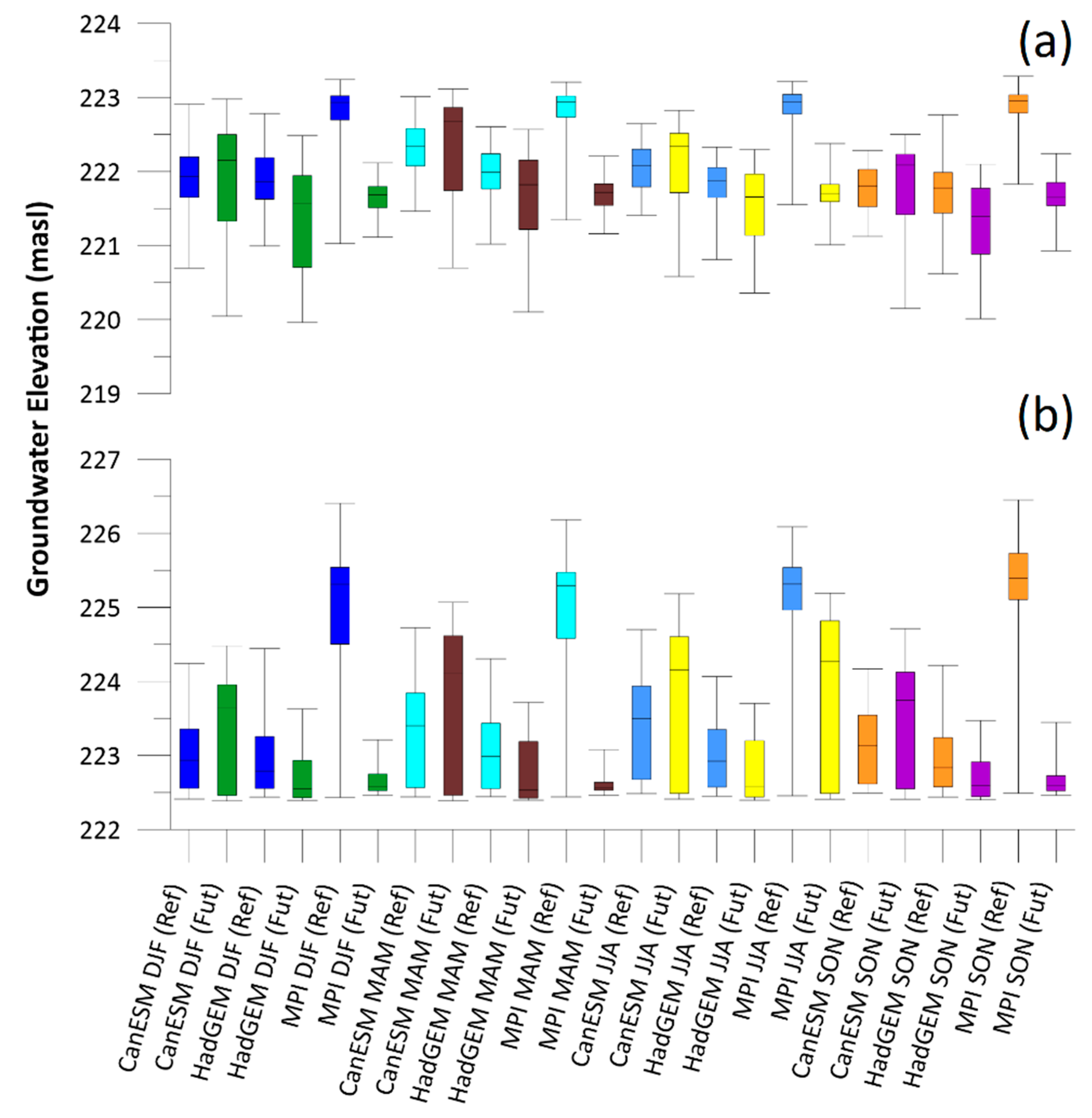
3.2.2. Groundwater Elevation

Modeling results of the groundwater elevations show that future groundwater elevations are generally lower, especially in the spring/summer periods (March to August) for the HadGEM and MPI climate change scenarios (Figure 8). However, the CanESM model increased water levels at the study site for future periods compared to the reference period at both monitoring wells (Figure 8). The groundwater elevation at two monitoring wells are discussed and presented in detail. The groundwater elevations for all climate change scenarios ranged between 220 masl and 223.5 masl at MW-04 (Figure 8a). The MPI (REF) scenario showed the highest increase in water elevation at MW-04 (Figure 8a). The groundwater elevation ranges between 222.5 masl and 226.5 masl for MPI for the reference period (Figure 8b). The groundwater elevations ranged between 222.5 m and 225 m for all climate change scenarios except MPI (REF) at MW-04 (Figure 8b). This might be due to high rainfall for the MPI model during the reference period compared to all other climate change models at the study site (Figure 6b). The MPI scenario for the future period showed the greatest decrease in groundwater elevation (based on the median) for both monitoring wells (Figure 8).

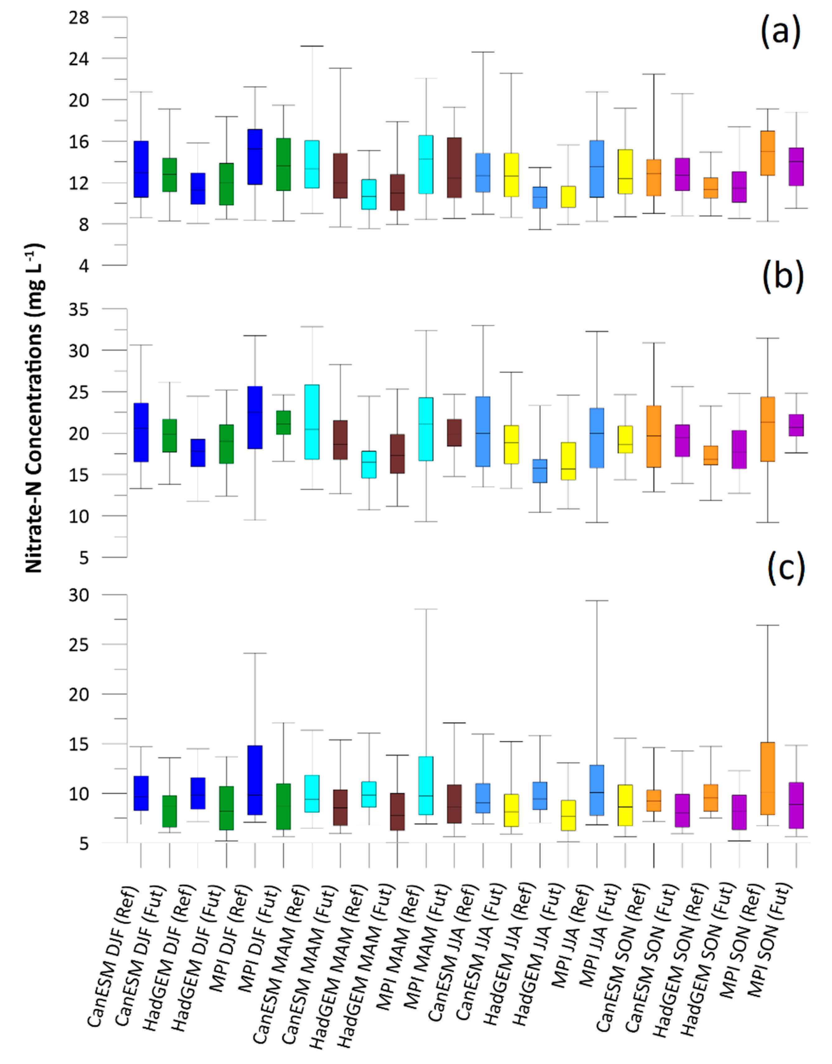
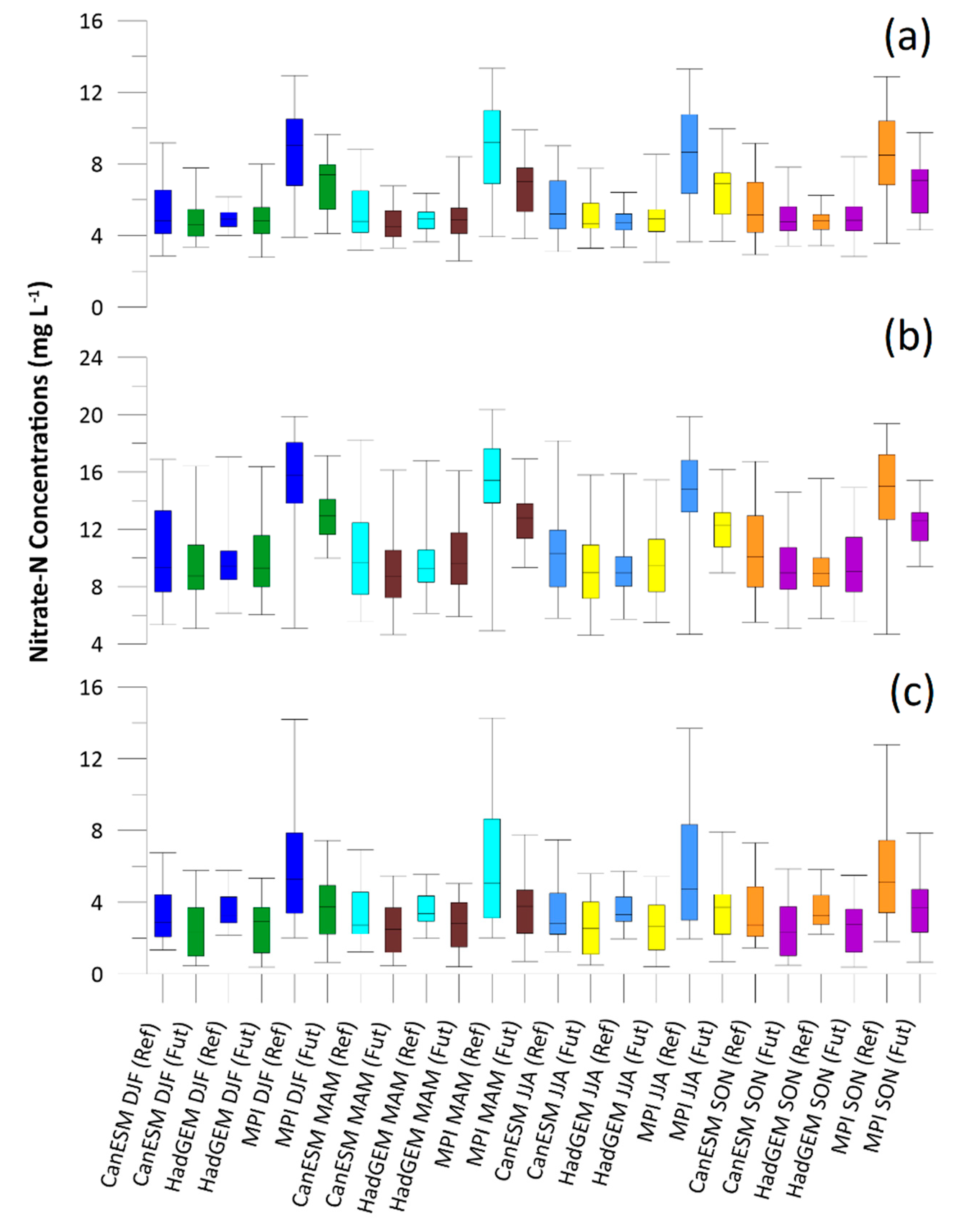
3.2.3. Groundwater Nitrate-N Concentrations

For the climate change scenarios and land use scenarios, the Nitrate-N concentration is generally lower for the future conditions at the study site (Figure 9). The Nitrate-N concentrations at MW-04 ranged between 8 to 26 mg L−1 for the corn-soybean land use scenario (Figure 9a), between 9 to 31 mg L−1 for the continuous corn land use scenario (Figure 9b), and between 5 to 29 mg L−1 for the BMP scenario (Figure 9c). At the MW-07 monitoring well, the Nitrate-N concentrations ranged between 3 to 13 mg L−1 for the corn-soybean land use scenario (Figure 10a), between 5 to 21 mg L−1 for the continuous corn land use scenario (Figure 10b), and between 1 to 13 mg L−1 for the BMP scenario (Figure 10c). The MPI scenario had the highest values for Nitrate-N concentrations for all three land use scenarios (Figure 10).
The model ensemble results at both MW-04 and MW-07 suggested a small increase of 0.02% and 0.16%, respectively, in groundwater elevation in the future period (Table 8). The groundwater elevation results were in contrast with outflow results when the reference period was compared with the future period, suggesting that groundwater elevations are less effected by future climate changes compared to outflows in the study sub-watershed (Table 7, Table 8 and Table 9).
The Nitrate-N concentrations were also decreased in the future model ensemble for all three land use and climate scenarios. The smallest reduction (0.14%) in Nitrate-N concentration was reported in MW-04 for the continuous corn scenario and the highest reduction (–47.36%) was reported in MW-07 for the BMP scenario (Table 8 and Table 9). The results of the comparison of different land use scenarios at the study site with corn-soybean as the base case scenario suggested that continuous corn production caused an increase of 47.56% and 79.43% during the reference period for MW-04 and MW07 respectively, while continuous corn production increased Nitrate-N concentrations by 51.21% and 89.52% in MW-04 and MW-07 respectively, for the future period (Table 8 and Table 9).
The likelihood of higher Nitrate-N concentrations in the groundwater in the future compared to the reference period is greater if continuous corn is planted (Table 8 and Table 9). The comparison of the base case scenario with the BMP scenario produced a reduction of 18.79% and 32.29% during the reference period for MW-04 and MW07, respectively (Table 8 and Table 9). Further, BMP adoption at the study site reduced Nitrate-N concentrations by 31.49% and 47.36% in MW-04 and MW-7 respectively, compared to the base case scenario for the future period (Table 8 and Table 9). The comparison of future and reference periods showed that adopting the BMP scenario (a rotation of corn-soybean-winter wheat-red clover) can have more positive impacts on groundwater quality in the future compared to the reference period (Table 8 and Table 9). The Nitrate-N concentrations are almost two times higher for continuous corn compared to the BMP scenario. Also, more extreme climate changes (e.g., the MPI scenario) can increase the risk of groundwater contamination under continuous cash crop production at the study site.

4. Discussion

The focus of this research was to predict the impact of different land use and climate change scenarios on groundwater elevations and Nitrate-N concentrations in a shallow, sandy aquifer setting in an agriculture-dominated sub-watershed in southern Ontario, Canada. Groundwater models were developed using HGS for the Norfolk site. The calibrated models were used to simulate reference (1986–2005) and future (2040–2059) surface water flows, groundwater elevations, and Nitrate-N concentrations in monitoring wells based on selected land use and climate change scenarios.
The selected climate change scenarios yielded lower Pnet values in the future period, which means less water is available for hydrologic processes. The model ensemble results indicated that the lower Pnet reduced the surface water flows significantly at the study site for the future period. A previous study conducted in Prince Edward Island (PEI), Canada [27] also produced a decrease in groundwater elevation for future climate change scenarios in agricultural lands. Another modeling study conducted in the same major watershed as the current study (Grand River watershed) resulted in a reduction in annual stream flow during the future (2040-2059) period compared to the reference period (1985-2005) [84]. The low annual Pnet values were the main reasons for lower streamflow and lower groundwater elevation. The findings of Reference [44] contrasted with the current study. Their results suggested an increase in groundwater discharge (spring flows) during the future period in a fractured bedrock aquifer of Chateauguay River watershed in Quebec, Canada. However, the Pnet values of the selected future climate change scenarios were higher compared to the reference period [44]. The future hydrologic water balance is highly dependent on study location and associated future climate model predictions.
The reduction in future Nitrate-N concentrations is in contrast with previous studies investigating groundwater or surface water quality conducted on agricultural lands [27,37,85,86]. These studies were based on increased nitrogen-based fertilizer application in future periods compared to reference periods. In the current study, a primary assumption was that current fertilizer application rates were also applied in the future periods. Only the impact of various land use scenarios (and their associated nitrogen application rates for the specific crops), including a BMP scenario, was studied. Therefore, the primary reason for lower nitrate concentrations observed in the modelled monitoring wells is less recharge (Pnet) which may result in less nitrate leaching from the surface. The lower nitrate concentrations can also mean that the nitrate could still be present in large amounts in the soil profile and can be leached down if precipitation occurs in higher amounts in the future. More research is needed to test climate change and land use change scenarios relating to nitrate impacts on groundwater from agricultural lands. The focus of this research was the comparison of land use change scenarios with similar inputs for reference and future periods. More numerical modelling studies are required to incorporate the changes in future nitrogen demands into these land use changes scenarios and to predict the impact on groundwater quality.

5. Conclusions

The numerical modeling results to represent outlet flow, groundwater elevation, and Nitrate-N concentrations for climate change and land use scenarios, showed: (1) a significant reduction in surface water flow in the future period, (2) a slight increase in groundwater elevation in the future period compared to the reference period at the study site, (3) a significant reduction in Nitrate-N concentrations in the future period compared to the reference period for all three climate change and all three land use scenarios if current fertilizer application rates are maintained, (4) a significant increase in groundwater Nitrate-N concentration (up to 80%) observed in monitoring wells if all the land under corn-soybean production is converted to continuous corn production for both reference and future periods, and (5) a significant reduction in Nitrate-N concentrations if the BMP scenario (corn-soybean-winter wheat-red clover rotation) is adopted at the study site for all three climate change scenarios during reference and future periods. The overall results suggest that BMPs should be adopted for unconsolidated hydrogeological settings to reduce potential impacts of Nitrate-N leaching on groundwater quality from agricultural lands. Planting of continuous corn along with the most extreme climate change scenario (MPI) can increase the risk of groundwater contamination.
Water managers and land use managers can use the results of this study and future similar studies in other jurisdictions to inform water protection and nutrient management policies in rural contexts to protect water at the source.

Author Contributions

The data collection, site conceptual model development, numerical modeling and analysis was performed by S.S. The original draft of the manuscript was written by S.S. Conceptualization, J.L.; methodology, J.L., B.P., R.M.; writing—review and editing, J.L., B.P., R.M.; supervision, J.L., B.P., R.M.; formal analysis, E.P.; project administration, J.L.; funding acquisition, J.L. All authors have read and agreed to the published version of the manuscript.

Funding

This research was funded by Ontario Ministry of Agriculture, Food and Rural Affairs; Grain Farmers of Ontario; Dairy Farmers of Ontario; Ontario Federation of Agriculture; Fertilizer Canada, and through an Ontario Graduate Scholarship.

Acknowledgments

The authors acknowledge Norfolk County for access to monitoring wells used in this study and Grand River Conservation Authority for data provision. The authors also acknowledge S. Berg at Aquanty Inc. for providing valuable HGS support, and H. Simpson, K. McKague, and B. Deen for advise regarding the future crop scenarios.

Conflicts of Interest

The authors declare no conflict of interest. The funders had no role in the design of the study; in the collection, analyses, or interpretation of data; in the writing of the manuscript, or in the decision to publish the results.

References

  1. Powlson, D.S.; Stirling, C.M.; Jat, M.L.; Gerard, B.G.; Palm, C.A.; Sanchez, P.A.; Cassman, K.G. Limited potential of no-till agriculture for climate change mitigation. Nat. Clim. Chang. 2014, 4, 678. [Google Scholar] [CrossRef]
  2. Rosenzweig, C.; Elliott, J.; Deryng, D.; Ruane, A.C.; Müller, C.; Arneth, A.; Boote, K.J.; Folberth, C.; Glotter, M.; Khabarov, N. Assessing agricultural risks of climate change in the 21st century in a global gridded crop model intercomparison. Proc. Natl. Acad. Sci. 2014, 111, 3268–3273. [Google Scholar] [CrossRef] [PubMed] [Green Version]
  3. Adams, R.M.; Hurd, B.H.; Lenhart, S.; Leary, N. Effects of global climate change on agriculture: An interpretative review. Clim. Res. 1998, 11, 19–30. [Google Scholar] [CrossRef] [Green Version]
  4. Risbey, J.; Kandlikar, M.; Dowlatabadi, H.; Graetz, D. Scale, context, and decision making in agricultural adaptation to climate variability and change. Mitig. Adapt. Strateg. Glob. Chang. 1999, 4, 137–165. [Google Scholar] [CrossRef]
  5. Pulido-Velazquez, M.; Peña-Haro, S.; García-Prats, A.; Mocholi-Almudever, A.F.; Henriquez-Dole, L.; Macian-Sorribes, H.; Lopez-Nicolas, A. Integrated assessment of the impact of climate and land use changes on groundwater quantity and quality in the Mancha Oriental system (Spain). Hydrol. Earth Syst. Sci. 2015, 19, 1677. [Google Scholar] [CrossRef] [Green Version]
  6. Danvi, A.; Giertz, S.; Zwart, S.J.; Diekkrüger, B. Comparing water quantity and quality in three inland valley watersheds with different levels of agricultural development in central Benin. Agric. Water Manag. 2017, 192, 257–270. [Google Scholar] [CrossRef]
  7. Carr, P.M.; Carlson, G.R.; Jacobsen, J.S.; Nielsen, G.A.; Skogley, E.O. Farming soils, not fields: A strategy for increasing fertilizer profitability. J. Prod. Agric. 1991, 4, 57–61. [Google Scholar] [CrossRef]
  8. Schumann, A.W.; Miller, W.M.; Zaman, Q.U.; Hostler, K.H.; Buchanon, S.; Cugati, S. Variable rate granular fertilization of citrus groves: Spreader performance with single-tree prescription zones. Appl. Eng. Agric. 2006, 22, 19–24. [Google Scholar] [CrossRef]
  9. Saleem, S.R.; Zaman, Q.U.; Schumann, A.W.; Madani, A.; Farooque, A.A.; Percival, D.C. Impact of variable rate fertilization on subsurface water contamination in wild blueberry cropping system. Appl. Eng. Agric. 2013, 29, 225–232. [Google Scholar] [CrossRef]
  10. Giller, K.E.; Tittonell, P.; Rufino, M.C.; Van Wijk, M.T.; Zingore, S.; Mapfumo, P.; Adjei-Nsiah, S.; Herrero, M.; Chikowo, R.; Corbeels, M. Communicating complexity: Integrated assessment of trade-offs concerning soil fertility management within African farming systems to support innovation and development. Agric. Syst. 2011, 104, 191–203. [Google Scholar] [CrossRef]
  11. Wu, W.; Ma, B. Integrated nutrient management (INM) for sustaining crop productivity and reducing environmental impact: A review. Sci. Total Environ. 2015, 512, 415–427. [Google Scholar] [CrossRef] [PubMed]
  12. Zingore, S.; Murwira, H.K.; Delve, R.J.; Giller, K.E. Influence of nutrient management strategies on variability of soil fertility, crop yields and nutrient balances on smallholder farms in Zimbabwe. Agric. Ecosyst. Environ. 2007, 119, 112–126. [Google Scholar] [CrossRef]
  13. Carpenter, S.R.; Bolgrien, D.; Lathrop, R.C.; Stow, C.A.; Reed, T.; Wilson, M.A. Ecological and economic analysis of lake eutrophication by nonpoint pollution. Aust. J. Ecol. 1998, 23, 68–79. [Google Scholar] [CrossRef]
  14. Powlson, D.S.; Addiscott, T.M.; Avery, A.A.; Van Kessel, C.; Davis, C. When Does Nitrate Become a Risk for Humans? J. Environ. Qual. 2008, 37, 291–295. [Google Scholar] [CrossRef] [Green Version]
  15. Van Drecht, G.; Bouwman, A.F.; Knoop, J.M.; Beusen, A.H.W.; Meinardi, C.R. Global modeling of the fate of nitrogen from point and nonpoint sources in soils, groundwater, and surface water. Glob. Biogeochem Cycles 2003, 17. [Google Scholar] [CrossRef]
  16. ECCC. Water Sources: Groundwater. Available online: https://www.canada.ca/en/environment-climate-change/services/water-overview/sources/groundwater.html (accessed on 15 September 2017).
  17. Gleeson, T.; Richter, B. How much groundwater can we pump and protect environmental flows through time? Presumptive standards for conjunctive management of aquifers and rivers. River Res. Appl. 2018, 34, 83–92. [Google Scholar] [CrossRef]
  18. Kurylyk, B.L.; MacQuarrie, K.T.B.; Linnansaari, T.; Cunjak, R.A.; Curry, R.A. Preserving, augmenting, and creating cold-water thermal refugia in rivers: Concepts derived from research on the Miramichi River, New Brunswick (Canada). Ecohydrology 2015, 8, 1095–1108. [Google Scholar] [CrossRef]
  19. Rhodes, K.A.; Proffitt, T.; Rowley, T.; Knappett, P.S.K.; Montiel, D.; Dimova, N.; Tebo, D.; Miller, G.R. The importance of bank storage in supplying baseflow to rivers flowing through compartmentalized, alluvial aquifers. Water Resour. Res. 2017, 53, 10539–10557. [Google Scholar] [CrossRef] [Green Version]
  20. ECCC. Canada at A Glance, Environment Edition: Water. Available online: https://www150.statcan.gc.ca/n1/pub/12-581-x/2017001/sec-1-eng.htm (accessed on 5 January 2018).
  21. Hutson, J.L.; Wagenet, R.J. Simulating nitrogen dynamics in soils using a deterministic model. Soil Use Manag. 1991, 7, 74–78. [Google Scholar] [CrossRef]
  22. Harbaugh, A.W.; Banta, E.R.; Hill, M.C.; McDonald, M.G. MODFLOW-2000, The U. S. Geological Survey Modular Ground-Water Model-User Guide to Modularization Concepts and the Ground-Water Flow Process; Open-File Report; U.S. Geological Survey: Reston, VA, USA, 2000. [CrossRef] [Green Version]
  23. Simunek, J.; Van Genuchten, M.T.; Sejna, M. The HYDRUS-1D software package for simulating the one-dimensional movement of water, heat, and multiple solutes in variably-saturated media. Univ. Calif.-Riverside Res. Rep. 2005, 3, 1–240. [Google Scholar]
  24. Youssef, M.A.; Skaggs, R.W.; Chescheir, G.M.; Gilliam, J.W. The nitrogen simulation model, DRAINMOD-N II. Trans. ASAE 2005, 48, 611–626. [Google Scholar] [CrossRef]
  25. Therrien, R.; McLaren, R.G.; Sudicky, E.A.; Panday, S.M. HydroGeoSphere: A three-dimensional numerical model describing fully-integrated subsurface and surface flow and solute transport; University of Waterloo: Waterloo, ON, Canada, 2010. [Google Scholar]
  26. Ma, L.; Ahuja, L.R.; Nolan, B.T.; Malone, R.W.; Trout, T.J.; Qi, Z. Root zone water quality model (RZWQM2): model use, calibration, and validation. Trans. ASABE 2012, 55, 1425–1446. [Google Scholar] [CrossRef]
  27. Paradis, D.; Vigneault, H.; Lefebvre, R.; Savard, M.M.; Ballard, J.; Qian, B. Groundwater nitrate concentration evolution under climate change and agricultural adaptation scenarios: Prince Edward Island, Canada. Earth Syst. Dyn. 2016, 7, 183–202. [Google Scholar] [CrossRef] [Green Version]
  28. Diersch, H.-J.G. FEFLOW: Finite Element Modeling of Flow, Mass and Heat Transport in Porous and Fractured Media; Springer Science & Business Media: Berlin, Germany, 2013. [Google Scholar] [CrossRef]
  29. Wagenet, R.J.; Hutson, J.L. LEACHM, a process-based model of water and solute movement, transformations, plant uptake and chemical reactions in the unsaturated zone. Contin 1989, 2. [Google Scholar]
  30. Graham, D.N.; Butts, M.B. Flexible, integrated watershed modelling with MIKE SHE. In Watershed Model; CRC Press: Boca Raton, FL, USA, 2005; pp. 245–272. [Google Scholar]
  31. Hansen, A.L.; Christensen, B.S.B.; Ernstsen, V.; He, X.; Refsgaard, J.C. A concept for estimating depth of the redox interface for catchment-scale nitrate modelling in a till area in Denmark. Hydrogeol. J. 2014, 22, 1639–1655. [Google Scholar] [CrossRef]
  32. Frey, S.K.; Hwang, H.; Park, Y.; Hussain, S.I.; Gottschall, N.; Edwards, M.; Lapen, D.R. Dual permeability modeling of tile drain management influences on hydrologic and nutrient transport characteristics in macroporous soil. J. Hydrol. 2016, 535, 392–406. [Google Scholar] [CrossRef]
  33. Praamsma, T.W. Rock Outcrops in the Canadian Shield: An Investigation of Contaminant Transport from Surface Sources in Fractured Rock Aquifers. Ph.D. Thesis, Queen’s University, Kingston, ON, USA, 2016. [Google Scholar]
  34. Wang, S.; Zhang, M.; Chen, F.; Che, Y.; Du, M.; Liu, Y. Comparison of GCM-simulated isotopic compositions of precipitation in arid central Asia. J. Geogr. Sci. 2015, 25, 771–783. [Google Scholar] [CrossRef] [Green Version]
  35. Allen, D.M.; Mackie, D.C.; Wei, M. Groundwater and climate change: A sensitivity analysis for the Grand Forks aquifer, southern British Columbia, Canada. Hydrogeol. J. 2004, 12, 270–290. [Google Scholar] [CrossRef]
  36. Levison, J.; Larocque, M.; Fournier, V.; Gagné, S.; Pellerin, S.; Ouellet, M.A. Dynamics of a headwater system and peatland under current conditions and with climate change. Hydrol. Processes 2014, 28, 4808–4822. [Google Scholar] [CrossRef] [Green Version]
  37. De Jong, R.; Qian, B.; Yang, J.Y. Modelling nitrogen leaching in Prince Edward Island under climate change scenarios. Can. J. Soil Sci. 2008, 88, 61–78. [Google Scholar] [CrossRef]
  38. Jiang, Y.; Somers, G. Modeling effects of nitrate from non-point sources on groundwater quality in an agricultural watershed in Prince Edward Island, Canada. Hydrogeol. J. 2009, 17, 707–724. [Google Scholar] [CrossRef]
  39. Colautti, D. Modelling the Effects of Climate Change on the Surface and Subsurface Hydrology of the Grand River Watershed. 2010. [Google Scholar]
  40. Sulis, M.; Paniconi, C.; Rivard, C.; Harvey, R.; Chaumont, D. Assessment of climate change impacts at the catchment scale with a detailed hydrological model of surface-subsurface interactions and comparison with a land surface model. Water Resour. Res. 2011, 47. [Google Scholar] [CrossRef]
  41. Sultana, Z.; Coulibaly, P. Distributed modelling of future changes in hydrological processes of Spencer Creek watershed. Hydrol. Process. 2011, 25, 1254–1270. [Google Scholar] [CrossRef]
  42. Dayyani, S.; Prasher, S.O.; Madani, A.; Madramootoo, C.A. Impact of climate change on the hydrology and nitrogen pollution in a tile-drained agricultural watershed in Eastern Canada. Trans. ASABE 2012, 55, 389–401. [Google Scholar] [CrossRef]
  43. Bourgault, M.A.; Larocque, M.; Roy, M. Simulation of aquifer-peatland-river interactions under climate change. Hydrol. Res. 2014, 45, 425–440. [Google Scholar] [CrossRef]
  44. Levison, J.; Larocque, M.; Ouellet, M.A. Modeling low-flow bedrock springs providing ecological habitats with climate change scenarios. J. Hydrol. 2014, 515, 16–28. [Google Scholar] [CrossRef] [Green Version]
  45. Bonton, A.; Bouchard, C.; Rouleau, A.; Rodriguez, M.J.; Therrien, R. Calibration and validation of an integrated nitrate transport model within a well capture zone. J. Contam. Hydrol. 2012, 128, 1–18. [Google Scholar] [CrossRef]
  46. Olesen, J.E.; Børgesen, C.D.; Hashemi, F.; Jabloun, M.; Bar-Michalczyk, D.; Wachniew, P.; Zurek, A.J.; Bartosova, A.; Bosshard, T.; Hansen, A.L. Nitrate leaching losses from two Baltic Sea catchments under scenarios of changes in land use, land management and climate. Ambio 2019, 48, 1252–1263. [Google Scholar] [CrossRef]
  47. Akbariyeh, S.; Pena, C.A.G.; Wang, T.; Mohebbi, A.; Bartelt-Hunt, S.; Zhang, J.; Li, Y. Prediction of nitrate accumulation and leaching beneath groundwater irrigated corn fields in the Upper Platte basin under a future climate scenario. Sci. Total Environ. 2019, 685, 514–526. [Google Scholar] [CrossRef]
  48. ECCC. Delhi Climate Station, Ontario. Available online: http://climate.weather.gc.ca (accessed on 3 January 2017).
  49. AAFC. Argiculture and Agri-Food Canada Annual Crop Inventory. Available online: https://open.canada.ca/data/en/dataset/ba2645d5-4458-414d-b196-6303ac06c1c9 (accessed on 6 May 2017).
  50. ONMNRF. Ontario Ministry of Natural resources and Forestry Provincial Digital Elevation Model (PDEM). Available online: https://www.javacoeapp.lrc.gov.on.ca/geonetwork/srv/en/main.home?uuid=012e3632-22a2-49d8-bbaf-ad8fbc0d0ceb (accessed on 4 June 2017).
  51. AquaResource, I. Long Point Region, Catfish Creek and Kettle Creek Integrated Water Budget. Report prepared for the Lake Erie Source Protection Region; AquaResources Inc.: Waterloo, ON, USA, 2009. [Google Scholar]
  52. Marich, A.S. An assessment of subsurface sediments in the Central Norfolk Sand Plain, Norfolk and Oxford Counties, Southern Ontario. Ont. Geol. Surv. Groundw. Resour. Study 2014, 14, 132. [Google Scholar]
  53. Karrow, P.F.; Dreimanis, A.; Barnett, P.J. A proposed diachronic revision of late Quaternary time-stratigraphic classification in the eastern and northern Great Lakes area. Quat. Res. 2000, 54, 1–12. [Google Scholar] [CrossRef]
  54. Singer, S.N.; Cheng, C.K.; Scafe, M.G. The hydrogeology of southern Ontario; Environmental Monitoring and Reporting Branch, Ministry of the Environment: Toronto, ON, Canada, 2003.
  55. Gardner, S. Groundwater Nitrate in Three Hydrogeologic Settings Throughout Southwestern Ontario. MASc Thesis, University of Guelph, Guelph, ON, Canada, 2017. [Google Scholar]
  56. Aravena, R.; Mayer, B. Isotopes and processes in the nitrogen and sulfur cycles. In Environmental Isotopes in Biodegradation and Bioremediation; CPC Press: Boca Raton, FL, USA, 2009; pp. 203–246. [Google Scholar]
  57. Saleem, S.R. Impacts of Future Climate and Agricultural Land Use Changes on Groundwater Nitrate Concentrations in Southern Ontario. Ph.D. Thesis, University of Guelph, Guelph, ON, Canada, 2018. [Google Scholar]
  58. Viessman, W.; Lewis, G.L. Introduction to Hydrology, 4th ed.; Harper Collins College Publisher: New York, NY, USA, 1996. [Google Scholar]
  59. HydroAlgorithemics Pty Ltd. What is AlgoMesh? HydroAlgorithemics Pty Ltd: Melbourne, Australia, 2017. [Google Scholar]
  60. Aquanty Inc. HydroGeoSphere Manual; Waterloo, ON, Canada, 2015. [Google Scholar]
  61. Richards, L.A. Capillary conduction of liquids through porous mediums. Physics 1931, 1, 318. [Google Scholar] [CrossRef]
  62. Kristensen, K.J.; Jensen, S.E. A model for estimating actual evapotranspiration from potential evapotranspiration. Hydrol. Res. 1975, 6, 170–188. [Google Scholar] [CrossRef] [Green Version]
  63. WSC. Daily Discharge Data Availability for LYNN RIVER AT SIMCOE (02GC008). Available online: https://wateroffice.ec.gc.ca/report/data_availability_e.html?type=historical&station=02GC008&parameter_type=Flow+and+Level (accessed on 24 January 2017).
  64. Stackhouse, P.W.; Westberg, D.; Hoell, J.M.; Chandler, W.S.; Zhang, T. Prediction Of Worldwide Energy Resource (POWER)—Sustainable Buildings Methodology—(1.0 o Latitude by 1.0 o Longitude Spatial Resolution). Available online: https://power.larc.nasa.gov/ (accessed on 9 June 2017).
  65. Doherty, J.E.; Hunt, R.J. Approaches to Highly Parameterized Inversion: A Guide to Using PEST for Groundwater-Model calibration; US Geological Survey: Washington, DC, USA, 2010.
  66. Chow, V.T. Open-channel hydraulics; McGraw-Hill: New York, NY, USA, 1959; Volume 1. [Google Scholar]
  67. Cochand, F. Impact des changements climatiques et du développement urbain sur les ressources en eaux du bassin versant de la rivière Saint-Charles. Ph.D. Thesis, Université Laval, Quebec City, QC, Canada, 2014. [Google Scholar]
  68. Goderniaux, P.; Brouyère, S.; Fowler, H.J.; Blenkinsop, S.; Therrien, R.; Orban, P.; Dassargues, A. Large scale surface–subsurface hydrological model to assess climate change impacts on groundwater reserves. J. Hydrol. 2009, 373, 122–138. [Google Scholar] [CrossRef]
  69. Scurlock, J.M.O.; Asner, G.P.; Gower, S.T. Worldwide historical estimates of leaf area index, 1932–2000; Oak Ridge National Laboratory: Oak Ridge, TN, USA, 2001. [Google Scholar] [CrossRef] [Green Version]
  70. Cornelissen, T.; Diekkrüger, B.; Bogena, H.R. Using high-resolution data to test parameter sensitivity of the distributed hydrological model HydroGeoSphere. Water 2016, 8, 202. [Google Scholar] [CrossRef] [Green Version]
  71. Canadell, J.; Jackson, R.B.; Ehleringer, J.B.; Mooney, H.A.; Sala, O.E.; Schulze, E.-D. Maximum rooting depth of vegetation types at the global scale. Oecologia 1996, 108, 583–595. [Google Scholar] [CrossRef]
  72. Li, Q.; Unger, A.J.A.; Sudicky, E.A.; Kassenaar, D.; Wexler, E.J.; Shikaze, S. Simulating the multi-seasonal response of a large-scale watershed with a 3D physically-based hydrologic model. J. Hydrol. 2008, 357, 317–336. [Google Scholar] [CrossRef]
  73. Andersen, J.; Dybkjaer, G.; Jensen, K.H.; Refsgaard, J.C.; Rasmussen, K. Use of remotely sensed precipitation and leaf area index in a distributed hydrological model. J. Hydrol. 2002, 264, 34–50. [Google Scholar] [CrossRef]
  74. Mercier, V.; Bussi, C.; Lescourret, F.; Génard, M. Effects of different irrigation regimes applied during the final stage of rapid growth on an early maturing peach cultivar. Irrig. Sci. 2009, 27, 297–306. [Google Scholar] [CrossRef]
  75. McCuen, R.H. The role of sensitivity analysis in hydrologic modeling. J. Hydrol. 1973, 18, 37–53. [Google Scholar] [CrossRef]
  76. Wang, X. Ontario Climate Change Data Portal. Available online: http://www.ontarioccdp.ca/ (accessed on 9 January 2018).
  77. Wang, G.; Yu, M.; Pal, J.S.; Mei, R.; Bonan, G.B.; Levis, S.; Thornton, P.E. On the development of a coupled regional climate–vegetation model RCM–CLM–CN–DV and its validation in Tropical Africa. Clim. Dyn. 2016, 46, 515–539. [Google Scholar] [CrossRef]
  78. Piani, C.; Haerter, J.O.; Coppola, E. Statistical bias correction for daily precipitation in regional climate models over Europe. Theor. Appl. Climatol. 2010, 99, 187–192. [Google Scholar] [CrossRef] [Green Version]
  79. Gutjahr, O.; Heinemann, G. Comparing precipitation bias correction methods for high-resolution regional climate simulations using COSMO-CLM. Theor. Appl. Climatol. 2013, 114, 511–529. [Google Scholar] [CrossRef]
  80. Wang, X.; Huang, G. Technical Report: Development of High-Resolution Climate Change Projections under RCP 8.5 Emissions Scenario for the Province of Ontario; IEESC, University of Regina: Regina, SK, Canada, 2015; pp. 1–90. [Google Scholar]
  81. Wang, L.; Ranasinghe, R.; Maskey, S.; van Gelder, P.H.A.J.M.; Vrijling, J.K. Comparison of empirical statistical methods for downscaling daily climate projections from CMIP5 GCMs: A case study of the Huai River Basin, China. Int. J. Climatol. 2016, 36, 145–164. [Google Scholar] [CrossRef]
  82. N’Tcha M’Po, Y.; Lawin, E.A.; Yao, B.K.; Oyerinde, G.T.; Attogouinon, A.; Afouda, A.A. Decreasing past and mid-century rainfall indices over the Ouémé River Basin, Benin (West Africa). Climate 2017, 5, 74. [Google Scholar] [CrossRef] [Green Version]
  83. Allen, R.G.; Pereira, L.S.; Raes, D.; Smith, M. Crop evapotranspiration-Guidelines for computing crop water requirements-FAO Irrigation and drainage paper 56. FaoRome 1998, 300, D05109. [Google Scholar]
  84. Golmohammadi, G.; Rudra, R.; Prasher, S.; Madani, A.; Mohammadi, K.; Goel, P.; Daggupatti, P. Water Budget in a Tile Drained Watershed under Future Climate Change Using SWATDRAIN Model. Climate 2017, 5, 39. [Google Scholar] [CrossRef] [Green Version]
  85. Dayyani, S.; Madramootoo, C.A.; Enright, P.; Simard, G.; Gullamudi, A.; Prasher, S.O.; Madani, A. Field evaluation of drainmod 5.1 under a cold climate: Simulation of daily midspan water table depths and drain outflows. J. Am. Water Resour. Assoc. 2009, 45, 779–792. [Google Scholar] [CrossRef]
  86. Juntakut, P.; Snow, D.D.; Haacker, E.M.K.; Ray, C. The long term effect of agricultural, vadose zone and climatic factors on nitrate contamination in the Nebraska’s groundwater system. J. Contam. Hydrol. 2019, 220, 33–48. [Google Scholar] [CrossRef]
Figure 1. Norfolk site: model domain boundary, elevation map [50], and land use map for Norfolk site for 2012 [49]. Red symbols indicate the positions of the monitoring wells (MWs) used in this study.
Sustainability 12 01153 g001
Figure 2. (a) Horizontal cross-sections (shown in plan view) to generate vertical cross-sections for model development at the study site. (b) Vertical cross-section (E-E’) (generated from Reference [51]) showing different hydrostratigraphic units.
Sustainability 12 01153 g002
Figure 3. Comparison of observed and modelled (a) groundwater elevation (meters above sea level (masl)) data and (b) Nitrate-N concentrations (mg L−1). Deviation from the 45° line indicates slight model under-prediction in both groundwater elevation and Nitrate-N concentrations’ calibrations.
Sustainability 12 01153 g003
Figure 4. Annual mean temperature and precipitation changes (reference to future period) for all climate change projections based on data downloaded from the Ontario Climate Change Data Portal (CCDP) for the RCP 8.5 emission scenario [76].
Sustainability 12 01153 g004
Figure 5. (a) Mean monthly temperature and (b) mean monthly precipitation for all climate change scenarios [76], model ensemble [76], and observed data at a local climate station (Delhi, Ontario).
Sustainability 12 01153 g005
Figure 6. Changes in monthly projected value of (a) temperature, (b) precipitation, and (c) Pnet for the 2040–2059 period at the study site for the three climate change model scenarios and the ensemble mean.
Sustainability 12 01153 g006
Figure 7. Outlfow (m3 s−1) observed at the outlet of the study site for different climate change scenarios. The 1st, 25th, 50th, 75th, and 99th percentiles are plotted. DJF (winter conditions (Dec, Jan, Feb)), MAM (spring conditions (Mar, Apr, May)), JJA (summer conditions (Jun, Jul, Aug)), and SON (fall conditions (Sep, Oct, Nov)). REF is the reference period (1986–2005) and FUT is the future period (2040–2059).
Sustainability 12 01153 g007
Figure 8. Groundwater elevation (masl) data for different climate change scenarios at (a) MW-04 and (b) MW-07 monitoring wells at the study site.
Sustainability 12 01153 g008
Figure 9. Nitrate-N concentration for different climate change scenarios under (a) corn-soybean rotation, (b) continuous corn, and (c) BMP (corn-soybean-wheat-red clover rotation) land use scenarios for the MW-04 monitoring well. The 1st, 25th, 50th, 75th, and 99th percentiles are plotted.
Sustainability 12 01153 g009
Figure 10. Nitrate-N concentration for different climate change scenarios under (a) corn-soybean rotation, (b) continuous corn, and (c) BMP (corn-soybean-wheat-red clover rotation) land use scenarios for the MW-07 monitoring well. The 1st, 25th, 50th, 75th, and 99th percentiles are plotted.
Sustainability 12 01153 g010
Table 1. Data types with spatial and temporal resolution used to simulate the model at the study site.
Data TypeSpatial ResolutionTemporal ResolutionMeasurement StationData Source
Norfolk Site
Climate DataWeather StationDailySimcoe[48]
Solar Radiation Data0.5° × 0.5°DailyPOWER Project [64]
DEM1 m × 1 m--GRCA
Subsurface GeologyLocal-Monitoring wells (borehole logs)[51]
OutflowOutflow StationDailyLynn River[63]
Table 2. Field estimates and calibrated values of hydraulic conductivities for different stratigraphic units at the study site. Field data values are from Reference [50].
Hydrostratigraphic UnitsCalibrated Kxy
(m s−1)
Calibrated Kz
(m s−1)
Field Data Range K
(m s−1)
Top Soil3.60 × 10−64.10 × 10−73.60 × 10−7 to 5.50 × 10⁻⁴
Norfolk Sand2.98 × 10−64.20 × 10⁻⁶
Norfolk Fine Sand 5.26 × 10−69.60 × 10−7
Interstadial Coarse Sediments1.32 × 10−61.00 × 10−69.80 × 10−8 to 1.70 × 10⁻³
Interstadial Fine Sediments1.89 × 10−69.60 × 10⁻⁷
Port Stanley Till2.80 × 10−72.80 × 10⁻⁷
Erie Phase Till1.35 × 10−71.35 × 10⁻⁷
Catfish Creek Till1.35 × 10−81.35 × 10⁻⁸
Palezoic Bedrock2.00 × 10−92.00 × 10⁻⁹
Table 3. Overland flow properties applied to the surface domain at the study site.
ParameterValueSource
Manning roughness coefficient, n (s m−1/3)0.025[66]
Rill storage height, Hd (m)0.01[67]
Coupling length0.01[68]
Table 4. Crop coverage, evapotranspiration, and surface flow parameters fixed during steady state calibration.
ParameterEvapotranspiration
Crop type
CerealsCornForestOther CropsSoybeansWetlandsDeveloped
Land use (%) (e.g. 2012)0.0516.328.321.725.32.06.5
Evaporation Depth (m)0.2 1
LAIDaily (RZWQM2)3.0 2Daily (RZWQM2)6.34 225.0 3
Root Depth (m)1.2 51.8 53.0 41.3 51.2 5--
Transpiration Fitting Parameters
(c1, c2, c3)
0.3 7, 0.15 7, 5.9 70.3 6, 0.2 6, 20.0 60.3 8, 0.4 8, 10 80.3 7, 0.2 7, 10.0 70.3 6, 0.2 6, 20.0 60.3 7, 0.2 7, 1.0 70.3 6, 0.2 6, 20.0 6
Transpiration Limiting Saturations
wp, θFC, θo, θao)
0.04, 0.19, 0.6 1, 0.8 10.04, 0.19, 0.76 9, 0.9 90.04, 0.19, 0.6 1, 0.8 10.04, 0.19, 1.0, 1.0
Evaporation Limiting Saturations
(min, max)
0.04, 0.19
Canopy Storage (mm)0.0562.5 30.8 30.05 61.5 315.0 315.0 3
1 Default values from References [60], 2 [69], 3 [70], 4 [71], 5 Mean values based on RZWQM outputs, 6 [72], 7 [62], 8 [73], 9 [74].
Table 5. Final values for different flow and transport parameters used for the transient state model at the study site.
Hydrostratigraphic UnitsLongitudinal Dispersivity (m)Transverse Dispersivity (m)TortuosityPorositySpecific Storage (m−1)
Top Soil20.01.230.0670.190.000328
Norfolk Sand23.632.000.0220.250.000321
Norfolk Fine Sand 8.490.90.0190.350.000164
Interstadial Coarse Sediments30.00.90.50.250.000298
Interstadial Fine Sediments30.02.00.50.450.000192
Port Stanley Till10.01.00.20.40.000164
Erie Phase Till10.01.00.20.40.000164
Catfish Creek Till10.01.00.20.40.000164
Palezoic Bedrock10.01.00.20.0010.000164
Table 6. Relative Sensitivity (Sr) of groundwater elevation, outflow, and groundwater Nitrate-N concentrations to changes in K, precipitation, and PET for steady state conditions.
ParameterGroundwater Elevation SrOutflow SrNitrate-N Sr
Low K (Layer 1–3)1.2 × 10−35.9 × 10−63.2 × 10⁻¹
High K (Layer 1–3)8.4 × 10−42.2 × 10−19.8 × 10⁻¹
Low K (Layer 4–5)2.9 × 10−46.6 × 10−65.8 × 10⁻⁷
High K (Layer 4–5)6.7 × 10−79.7 × 10−75.9 × 10⁻⁷
Low Precipitation1.5 × 10−29.0 × 10−11.5 × 100
High Precipitation2.2 × 10−28.2 × 10−18.9 × 10−1
Low PET8.9 × 10−44.8 × 10−23.5 × 10−1
High PET5.5 × 10−43.5 × 10−28.1 × 10−2
Table 7. Comparison of outflow changes between the reference and future model ensembles at the study site.
PeriodOutflow (m3 s−1)% Change
1986–2005 1.12 a−2.86
2040–20591.09 b
Note: Means followed by different letters (a versus b) are significantly different at a significance level of 0.05.
Table 8. Comparison of groundwater elevation (masl) and Nitrate-N concentration (mg L−1) changes between the reference and future model ensembles at the MW-04 monitoring well. Changes between different land uses are compared to a corn-soybean rotation as the base case scenario.
Parameter1986–20052040–2059% Change% Change between Land Uses
(1986–2005)(2040–2059)
Groundwater elevation (masl)222.00 a222.05 b+0.02-
Corn-soybean (mg L−1)13.00 a12.67 b−2.55
Continuous corn (mg L−1)19.19 a19.16 b−0.14+47.56+51.21
Corn-soybean-winter wheat-red clover (mg L−1)10.56 a8.68 b−17.78−18.79−31.49
Note: Means followed by different letters (a versus b) are significantly different at a significance level of 0.05.
Table 9. Comparison of groundwater elevation (masl) and Nitrate-N concentration (mg L−1) changes between the reference and future model ensembles at the MW-07 monitoring well. Changes between different land uses are compared to a corn-soybean rotation as the base case scenario.
Parameter1986–20052040–2059% Change% Change between Land Uses
(1986–2005)(2040–2059)
Groundwater elevation (masl)223.24 a223.60 b+0.16--
Corn-soybean (mg L−1)6.30 a5.51 b−12.45
Continuous corn (mg L−1)11.30 a10.45 b−7.53+79.43+89.52
Corn-soybean-winter wheat-red clover (mg L−1)4.26 a2.90 b−31.93−32.29−47.36
Note: Means followed by different letters (a versus b) are significantly different at a significance level of 0.05.

